Line–Household Relationship Identification Method for a Low-Voltage Distribution Network Based on Voltage Clustering and Electricity Consumption Characteristics

Abstract

To address the issue of inconspicuous electricity consumption characteristics among vacant users in low-voltage distribution networks (LVDNs), which hinders effective line–household relationship identification (LHRI), a method for identifying line–household relationship based on voltage clustering and electricity consumption characteristics is proposed. Initially, the paper employs Dynamic Time Warping (DTW) to analyze the similarity of user voltage profiles and utilizes the Density-Based Spatial Clustering of Applications with Noise (DBSCAN) algorithm to cluster users. This approach identifies the topological relationship between vacant users and regular users to obtain multiple user categories. Subsequently, by analyzing the electricity consumption characteristic, the connection relationships between different user categories and phase lines are clarified based on the correlation between the electricity consumption characteristic vector of phase lines and the electricity consumption characteristic vector of user categories, thereby revealing the line–household relationship for all users. On the test dataset, the LHRI algorithm proposed in this article achieved 100% accuracy, within an allowable error range of 0.2%, and improved the accuracy by 20% compared to the traditional identification method. Finally, the LVDN simulation model established by OpenDSS 9.4.0.3 was used to verify the effectiveness of the proposed method, confirming its potential and advantages in practical applications.

1. Introduction

As the demand for high-quality power supply among users increases, resolving the chaotic end topology information in LVDNs is crucial for optimizing the power supply network and improving operational quality and efficiency [1,2]. For a long time, due to a large number of devices in distribution networks and low levels of automation, the accuracy and completeness of the line–household relationship in topology archives have been relatively low. This has significantly hindered the management of issues such as three-phase imbalance [3] and line loss [4], and other advanced applications. Furthermore, as distributed energy sources increasingly integrate into the power system, LVDNs require more sophisticated operational management, making it especially important to obtain accurate and real-time line–household structures [5]. Reliance on manual field inspections and the organization of substation topologies is inefficient and fails to achieve digital storage for topology archives.

The current methods for distribution network topology identification mainly include signal injection and data analysis. The signal injection method involves installing communication devices or handheld substation identifiers in the distribution network. Electrical connection relationships are identified by analyzing feedback signals from terminal devices [6,7]. This method generally offers a relatively high identification rate in specific circuits, but it requires additional terminal equipment, resulting in higher investment and maintenance difficulties, and has high demands for signal processing.

The data analysis method refers to the optimization of distribution network systems using measurement data from advanced metering systems [8]. With the deepening of the “Internet+” strategy and the accelerated digital transformation of intelligent power systems, advanced metering infrastructure (AMI) has achieved significant success in its widespread adoption and promotion in distribution networks. The AMI system can measure key electrical parameters, such as electricity, voltage, and current, in real time, greatly facilitating power companies in the collection of grid operation data and user electrical measurements. This provides a solid information base for analyzing the grid’s topological structure [9]. Hence, the data analysis method has increasingly become an important approach for domestic and international scholars in researching the identification and verification of distribution network line–household relationships [10,11,12,13]. In [10], incorrectly connected users within the transformer neighborhood are detected and corrected based on the correlation coefficient and relative amplitude level of the hourly voltage distribution. In [11], based on the distribution characteristics of the distribution network voltage and combined with the correlation analysis method, the feeder to which each load belongs is determined, and then the upstream and downstream relationships of each load in the feeder are verified based on the amplitude of the node voltage in the feeder. The topological connection relationships of the distribution network are recorded by the geographic information system. In [12], based on the time series of voltage measurements at homes and distribution transformers, the correlation between the voltage curve of the smart meter and the voltage curve of the distribution transformer is analyzed to determine the phase connection relationship of the user. In [13], a phase sequence identification method that adds FisherZ transformation based on the harmonic voltage correlation coefficient is proposed. However, these studies have not yet covered the identification of line–household relationship attribution.

With economic development and the popularization of distributed energy sources, vacant users [14] with no electricity consumption on non-holidays are ubiquitous, and the peak electricity demand during holidays mainly comes from these vacant users. To manage peak power demand, it is necessary to stage-connect vacant users. Compared to regular users, the electricity consumption characteristics of vacant users are not prominent, making traditional identification methods based on current features, load curves, and load sequence correlations ineffective in revealing their line–household relationship. Moreover, in the process of collecting electrical data, the presence of measurement errors is inevitable.

Therefore, to address the presence of vacant users, measurement errors, and missing line–household information in LVDNs, this paper proposes a method for identifying line–household relationships based on voltage clustering and electricity consumption characteristics. Initially, user clustering analysis is conducted by utilizing the DTW algorithm in combination with the DBSCAN algorithm, based on the similarity of user voltage time-series curves. Through this analysis, the line–household relationship of vacant users and regular users can be effectively associated, leading to the obtainment of multiple different user categories. Subsequently, based on the feature extraction of the electricity consumption sequence, the connection relationships between different user categories and phase lines are clarified based on the correlation between the electricity consumption characteristic vector of phase lines and the electricity consumption characteristic vector of user categories, thereby revealing the line–household relationship for all users. This enables comprehensive identification of the line–household relationship for all users in the substation area. Finally, an LVDN simulation model is constructed using OpenDSS 9.4.0.3 to verify the effectiveness and accuracy of the proposed method.

2. Principles of LHRI in LVDNs

2.1. LVDN Topology

The typical topology of an LVDN is illustrated in Figure 1. It consists of a radial structure formed by distribution transformers, lines, and multiple load points. The branch feeders (primary branch lines) are mostly laid in a three-phase four-wire system, delivering electrical energy to the users of each phase through low-voltage meter boxes. Considering the uniqueness of the connection relationship between the users and the phases of the branch feeders (referred to as “phase lines”), this paper describes the process of identifying the affiliation relationship between phase lines and users as LHRI.

Based on the characteristics of LVDNs, the research method of this paper mainly includes the following two aspects:

(1)

A user clustering method based on voltage characteristics. In LVDNs, regardless of how much electric energy a user consumes, the voltage data recorded by their smart electricity meters always remain within a specific range. The voltage at adjacent nodes is significantly affected by the initial voltage of the line in the substation area, line impedance, and the active and reactive power flowing through it. Given that low-voltage distribution systems usually include reactive power compensation devices, the impact of reactive power on voltage can be relatively neglected. The shorter the electrical distance, the more similar the initial voltage of the line, line impedance, and active power values within the substation area, leading to more similar voltage variation trends between adjacent nodes. Therefore, within the same substation area, users located on the same line exhibit highly similar voltage time-series curves, and the shorter the electrical distance, the more pronounced this similarity. Conversely, users on different lines show greater differences in their voltage time-series curves. Based on this, this paper proposes a clustering method based on voltage similarity to explore and reconstruct the connection relationships between vacant users and regular users. The key to clustering is the aggregation of users through voltage data, rather than individual analysis, to solve the problem of identifying vacant users. Importantly, the purpose of clustering is to identify the overall connections between users in the power grid, rather than pursuing extreme accuracy, thereby effectively bundling user groups.

(2)

An identification method based on electricity consumption characteristics. Within a certain period, when there is a significant increase or decrease in the electricity consumption of a user category, the electricity consumption of the connected phase line also increases or decreases correspondingly. Therefore, this paper identifies the phase line to which a user category belongs by accurately extracting key features from the electricity consumption sequence data of the user category and analyzing its correlation with the phase line electricity consumption.

2.2. User Voltage Curve Similarity Measurement

When dealing with inconsistent lengths of voltage time series or missing data, the DTW algorithm [15] can calculate the minimum distance between sequences through the dynamic bending of the voltage time series, thereby effectively capturing and highlighting the subtle fluctuations in the voltage time-series curve and its overall difference. Based on this, this article uses DTW distance as a metric to evaluate the similarity between user voltage timing curves. That is, the smaller the DTW distance, the higher the similarity of the voltage timing curves of two users, and the more likely they are to be on the same line.

Assuming within the same low-voltage substation area, the voltage time series of any two users are represented as $X=\left\{x_1,x_2,\cdots ,x_i,\cdots ,x_m\right\}$ and $Y=\left\{y_1,y_2,\cdots ,y_j,\cdots ,y_n\right\}$, here, $x_i$ represents the voltage value of the $i$-th data point in series $X$; $y_j$ represents the voltage value of the $j$-th data point in series $Y$; and $m$ and $n$ are the respective lengths of series $X$ and $Y$. The specific quantification process is as follows:

(1)

Calculate the Euclidean distance between x_i and y_i to form a distance matrix $D$. The values of each element in the matrix are calculated using Equation (1).

$$D_{i,j}={(x_i-y_j)}^2$$

(1)

where $D_{i,j}$ represents the value of the element in the $i$-th row and $j$-th column of the distance matrix $D$.

(2)

Construct the cumulative distance matrix $\mathit{C}$, where $C_{i,j}$ represents the minimum cumulative distance from $x_i$ to $y_j$. This is calculated using Equation (2).

$$C_{i,j}=D_{i,j}+\min \{\begin{array}{c}{C}_{i,j-1}\\ C_{i-1,j-1}\\ C_{i-1,j}\end{array}$$

(2)

(3)

where $i=1,2,\cdots ,m$, $j=1,2,\cdots ,n$, $C_{0,0}=0$, and $C_{i,0}=C_{0,j}=+\infty$. The final element value $C_{m,n}$ in the cumulative distance matrix $\mathit{C}$ is the DTW distance calculated based on the fluctuation trend of the voltage curve.

$$\mathrm{DTW}(X,Y)=C_{m,n}$$

(3)

where $\mathrm{DTW}(X,Y)$ is the function used to calculate the distance between voltage sequences $X$ and $Y$.

2.3. User Clustering Analysis Based on DTW Distance

After measuring the similarity of user voltage time-series curves using DTW distance, it is difficult to set an appropriate threshold to judge whether vacant users and regular users belong to the same phase line. The DBSCAN algorithm [16] has the advantage of not requiring the manual setting of the number of clusters and can automatically determine the number of clusters based on the spatial density of samples, making it suitable for datasets of any shape. Therefore, this section uses the DBSCAN algorithm to cluster substation users based on the DTW distance between user voltage sequences, topologically associating vacant users with regular users on the same phase line, and laying the groundwork for further refinement in identifying line–household relationships.

The choice of two parameters, epsilon $p$ and minimum samples $q$, has a significant impact on the accuracy of the DBSCAN clustering results. To avoid this impact, $p$ is set to vary from 0 to $p*$ in increments of 0.1, and $q$ is set to vary from 2 to $q*$ in increments of 1, where $p*$ and $q*$ are the optimal values for $p$ and $q$, respectively. For each parameter combination, run DBSCAN and calculate the silhouette score. Finally, select the parameter combination with the highest silhouette score as the optimal parameters for the DBSCAN clustering algorithm.

When conducting clustering analysis, the users in the substation area are numbered. Taking the voltage time series of any user as the center and $p$ as the radius, a circle is drawn. The DTW distance is used to measure the distance between the voltage time series of nodes. Then, the user data within each circle are counted to check whether they meet the density threshold $q$. If the density threshold condition is met, these users are classified into one group. By deriving the user set with the highest density connection through density relationships, it is treated as a clustering category. This process is repeated until the categories of all users, except for noise points, are determined.

Further clustering is conducted for users who are the sole members of a category in the clustering results. Specifically, these solitary users are clustered into the category that has the smallest DTW distance value to them. Ultimately, a set of user categories $G=\left\{1,2,\cdots ,H\right\}$ is obtained, where $H$ represents the total number of user clustering categories in the set $G$, completing the user clustering process.

Based on the comprehensive analysis, by leveraging the electrical characteristics of low-voltage distribution systems and measuring the similarity of voltage curves, clustering analysis can effectively establish the topological association between vacant users and regular users.

2.4. Analysis of Line–Household Electricity Consumption Time-Series Characteristics

It should be noted that within the user clustering set $G$, multiple users of the same category obtain electrical energy from the same phase line; therefore, individual user line–household information can be reflected by the user category. To reduce the number of variables in subsequent studies on LHRI, users with consistent line–household relationships are merged into the same user category. That is, at the same moment in time, the electricity consumption of users clustered in the same category is summed up, and the summation is taken as the electricity value for that user category at that moment in time.

$$Q_{ht}^{\mathrm{clu}}=\sum _{u\in G\left(h\right)}{Q}_{ut}h\in G, t\in \beta$$

(4)

where $Q_{ht}^{\mathrm{clu}}$ represents the sum of electricity values of all users in category $h$ at moment $t$; $\beta =\left\{1,2,\cdots ,T\right\}$ is the set of time slices of the measured dataset; and $Q_{ut}$ is the electricity value of user $u$ at moment $t$. From this, the electricity time series for all user categories can be obtained.

To visually represent the electricity values of different user categories at various times, construct a user category electricity matrix ${\mathit{Q}}^{\mathrm{clu}}$.

$$Q^{\mathrm{clu}}=\left[\begin{array}{cccccc}{Q}_{11}^{\mathrm{clu}}& Q_{12}^{\mathrm{clu}}& \cdots & Q_{1t}^{\mathrm{clu}}& \cdots & Q_{1T}^{\mathrm{clu}}\\ Q_{21}^{\mathrm{clu}}& Q_{22}^{\mathrm{clu}}& \cdots & Q_{2t}^{\mathrm{clu}}& \cdots & Q_{2T}^{\mathrm{clu}}\\ ⋮& ⋮& \ddots & ⋮& \ddots & ⋮\\ Q_{h1}^{\mathrm{clu}}& Q_{h2}^{\mathrm{clu}}& \cdots & Q_{ht}^{\mathrm{clu}}& \cdots & Q_{hT}^{\mathrm{clu}}\\ ⋮& ⋮& \ddots & ⋮& \ddots & ⋮\\ Q_{H1}^{\mathrm{clu}}& Q_{H2}^{\mathrm{clu}}& \cdots & Q_{Ht}^{\mathrm{clu}}& \cdots & Q_{HT}^{\mathrm{clu}}\end{array}\right]$$

(5)

For the convenience of analysis, let the matrix composed of the electricity consumption of each phase line be denoted as $Q^{\mathrm{L}}$.

$$Q^{\mathrm{L}}={\left[\begin{array}{cccccc}{Q}_1^{\mathrm{L}}& Q_2^{\mathrm{L}}& \cdots & Q_e^{\mathrm{L}}& \cdots & Q_E^{\mathrm{L}}\end{array}\right]}^{\mathrm{T}}$$

(6)

$$Q_e^{\mathrm{L}}=\left[\begin{array}{cccccc}{Q}_{e1}^{\mathrm{L}}& Q_{e2}^{\mathrm{L}}& \cdots & Q_{et}^{\mathrm{L}}& \cdots & Q_{eT}^{\mathrm{L}}\end{array}\right]$$

(7)

where $Q_e^{\mathrm{L}}$ represents the electricity consumption series of phase line $e$; $Q_{et}^{\mathrm{L}}$ is the electricity value of phase line $e$ at moment $t$; and $E$ denotes the total number of outgoing lines on the low-voltage side.

2.4.1. Feature Extraction of User Category Electricity Consumption

Feature extraction involves identifying the more prominent changing points in the electricity consumption of user categories. This is achieved by calculating the electricity consumption changes between any two sampling moments, highlighting the electricity characteristics of the user categories. By taking the difference between any two columns of ${\mathit{Q}}^{\mathrm{clu}}$ from Equation (5), a user category electricity consumption change matrix $Q^{\mathrm{CV}}$ is constructed, with the number of columns $V$ calculated using Equation (8). From the perspective of the data used, the focus is on the changes in electricity values, rather than the electricity values themselves.

$$V=(T-1)+(T-2)+\cdots +1=T(T-1)/2$$

(8)

$$Q^{\mathrm{CV}}={\left[\begin{array}{cccccc}{Q}_1^{\mathrm{CV}}& Q_2^{\mathrm{CV}}& \cdots & Q_h^{\mathrm{CV}}& \cdots & Q_H^{\mathrm{CV}}\end{array}\right]}^{\mathrm{T}}$$

(9)

where $Q_h^{\mathrm{CV}}$ is the vector of electricity consumption changes for user category $h$.

Within the same time step, if the electricity consumption change in a certain user category is significantly higher than the sum of changes in other categories, then this change is defined as significant change [17]. To illustrate the process, take user category $h$ as an example for analysis. Significant change points in electricity consumption are captured through Formula (10).

$$\left|Q_h^{\mathrm{CV}}(v)\right|\ge \lambda \sum _{d>h}^H{Q}_d^{\mathrm{CV}}(v)$$

(10)

where $Q_h^{\mathrm{CV}}(v)$ is the $v(v=1,2,\cdots ,V)$-th electricity consumption change feature point of user category $h$; the numerical value $\lambda$ is a threshold to adjust the significance level of the change, which is a number not less than 1 and can be adjusted according to the data situation [17]; and $Q_d^{\mathrm{CV}}(v)$ is the electricity consumption change value of user category $d$ at the $v$-th time. To further highlight the differences and uniqueness between the electricity consumption sequences of different user categories, on top of the sequence formed by the above-mentioned feature points, the extremal points of the feature sequence are extracted, as calculated by Formula (11).

$$Q_h^{\mathrm{CV}}(w)=\max /\min \left[Q_h^{\mathrm{CV}}(w-1),Q_h^{\mathrm{CV}}(w),Q_h^{\mathrm{CV}}(w+1)\right]$$

(11)

where $Q_h^{\mathrm{CV}}(w)$ is the $w\left(2<w<V-1\right)$ feature point of user category $h$, which reflects the significant changes and fluctuation characteristics of the electricity consumption sequence of the user category. Assuming that the total number of feature points extracted from sequence $Q_h^{\mathrm{CV}}$ is $N$, the feature vector for user category $h$ is $Q_h^{\mathrm{CX}}$, as shown in Equation (12).

$${\mathit{Q}}_h^{\mathrm{CX}}=\left[Q_h^{\mathrm{CX}}\left(1\right),Q_h^{\mathrm{CX}}\left(2\right),\cdots ,Q_h^{\mathrm{CX}}\left(s\right),\cdots ,Q_h^{\mathrm{CX}}\left(N\right)\right]$$

(12)

where $Q_h^{\mathrm{CX}}$ is the $s$-th feature point of the electricity consumption sequence of the characteristic user category $h$.

2.4.2. Feature Vector Correlation Analysis

In the above-mentioned steps, the feature vector of electricity consumption for the user category $h$ is obtained through feature extraction. Concurrently, using Equation (6), feature points corresponding to all phase line electricity consumption series and the electricity of the user category h can also be extracted. Analyzing the correlation between the electricity feature vector of user category h and all phase lines can identify the phase line to which that user category is connected. Therefore, the Pearson correlation coefficient [18] is used to measure the similarity of feature vectors. Taking the electricity of user category h and phase line $e$ as an example, the correlation formula for their feature vectors $Q_h^{\mathrm{CX}}$ and $Q_e^{\mathrm{LX}}$ is as follows:

$$r_{he}=\frac{{\displaystyle \sum _{s=1}^N\left(Q_h^{\mathrm{CX}}\left(s\right)-Q_h^{\prime \mathrm{CX}}\right)}\left(Q_e^{\mathrm{LX}}\left(s\right)-Q_e^{\prime \mathrm{LX}}\right)}{\sqrt{{\displaystyle \sum _{s=1}^N{\left(Q_h^{\mathrm{CX}}\left(s\right)-Q_h^{\prime \mathrm{CX}}\right)}^2}}\sqrt{{\displaystyle \sum _{s=1}^N{\left(Q_e^{\mathrm{LX}}\left(s\right)-Q_e^{\prime \mathrm{LX}}\right)}^2}}}$$

(13)

where $r_{he}$ is the correlation coefficient value between feature vectors $Q_h^{\mathrm{CX}}$ and $Q_e^{\mathrm{LX}}$. $Q_h^{\prime \mathrm{CX}}$ and $Q_e^{\prime \mathrm{LX}}$ represent the average values of sequences $Q_h^{\mathrm{CX}}$ and $Q_e^{\mathrm{LX}}$, respectively.

Repeat the above steps to obtain the Pearson correlation coefficient matrix $A$ between the electricity consumption characteristic vector of all user categories and the electricity consumption characteristic vector of all phase lines, as shown below.

$$A=\left[\begin{array}{cccccc}{r}_{11}& r_{12}& \cdots & r_{1e}& \cdots & r_{1E}\\ r_{21}& r_{22}& \cdots & r_{2e}& \cdots & r_{2E}\\ ⋮& ⋮& & ⋮& & ⋮\\ r_{h2}& r_{h2}& \cdots & r_{he}& \cdots & r_{hE}\\ ⋮& ⋮& & ⋮& & ⋮\\ r_{H2}& r_{H2}& \cdots & r_{He}& \cdots & r_{HE}\end{array}\right]$$

(14)

In row vector $A_h$, if the value of element $A_{he}$ is the largest, then the electricity consumption characteristics of user category $h$ have the greatest correlation with the electricity consumption characteristics of phase line $e$. That is, phase line $e$ is the attributed phase line of user category $h$. Users included in user category $h$ are also dependent on this phase line. Thus, the affiliation relationship between all users in this station area and their phase lines is obtained.

In order to explore the effectiveness of the LHRI algorithm, the accuracy rate (accuracy rate = number of correctly identified users/total number of users in LVDN) is used as an indicator of evaluation results. Based on the above recognition results, the adjacency matrix $\mathit{B}$ is established. If there is a connection relationship between user $c$ and phase line $e$, then the element $B_{ce}=1$; otherwise, $B_{ce}=0$. Matrix $\mathit{B}$ is compared with the adjacency matrix established based on the actual line–household connection relationship in the LVDN to obtain the accuracy of the algorithm proposed in this article.

3. LHRI Algorithm Flow

The specific implementation steps of the LVDN LHRI algorithm based on voltage clustering and electricity consumption characteristics are as follows:

• Import historical voltage time-series data from smart electricity meters of low-voltage power distribution network consumers.
• Calculate the DTW distance between voltage time series.
• Cluster users based on DTW distance using the DBSCAN algorithm.
• Users classified as noise points are clustered into the category with which they have the smallest DTW distance value.
• Import historical electricity consumption time-series data for phase lines and users in the LVDN.
• Aggregate electricity consumption for each user category and extract feature points to form a characteristic vector.
• Calculate the Pearson correlation coefficient between the electricity consumption characteristic vectors of user categories and the characteristic vectors of the phase lines; select the largest value to identify the corresponding phase line, thereby obtaining the line–household relationship of the LVDN.

The algorithmic procedure for LHRI is illustrated in Figure A1.

4. Case Study

4.1. Case Study Setup

To verify the effectiveness of the identification algorithm, a low-voltage power distribution network simulation model was established in the LVDN simulation software OpenDSS 9.4.0.3 [19,20], with the line–household relationship and line data parameters as shown in Figure A2.

The system includes 103 users, among which the three-phase users T1, T2, and T3 can be regarded as single-phase users T1A, T1B, T1C, T2A, T2B, T2C, T3A, T3B, and T3C, respectively. Thus, the users to be identified can be considered as 109 single-phase users. Users U5, U23, U30, U55, U82, and U89 are randomly set as vacant users, totaling five. The system contains nine phase lines, which are 1.1A, 1.1B, 1.1C, 1.2A, 1.2B, 1.2C, 1.3A, 1.3B, and 1.3C. Through case analysis, this study validates the effectiveness of the proposed method by identifying the connection relationships between 109 users and 9 phase lines.

During the construction of the simulation model, the electricity consumption data of 109 customers from a regional power distribution network were used as input. A three-phase, four-wire system load flow calculation method was employed to obtain the measurements from branch units and customer smart meters. Considering that some distribution areas have undergone three-phase imbalance remediation, the impact of load fluctuations within these areas on the root node voltage is approximately neglected, setting the transformer’s low-voltage side as a balanced node. To better match the flow distribution of the test system, the power factor of the customers is maintained between 0.93 and 0.97. The test data consist of 96 steady-state data samples collected at a 15 min interval each day. To simulate real-world conditions, error modeling is achieved by adding Gaussian noise of different levels to the output dataset. For each level of error, random experiments incorporating noise are simulated using the Monte Carlo method, and their average values are taken to assess the identification performance of the algorithm proposed in this article in noisy datasets.

Regarding the specific identification process, the test case encompasses four main aspects: Firstly, the identification process results of the proposed method are given, and then a comparative analysis is conducted with existing methods. Then, a sensitivity analysis of two indicators, measurement error, and data length is carried out.

4.2. User Clustering Results

To validate the association between vacant users and regular users, a 10-day simulation sample dataset was selected for study, with the measurement error set at 0.2%. By adopting the silhouette score to assess the sensitivity of DBSCAN parameters, the parameter combination with the highest evaluation score is selected as the optimal parameter. As shown in Figure A3, the minimum number of samples required to form a cluster is set to 2, and the epsilon is set to 1. The obtained clustering visualization results are shown in Figure 2, where different colors represent different user categories, and points labeled with −1 represent noise points. The horizontal and vertical coordinates correspond to the dimensions after feature reduction.

According to Figure 2, the 109 users are classified into 25 user categories and one noise point, U101, after clustering. As depicted in Figure A2, users U7 to U12 have similar topological relationships, and their distance from U101 (T1) is over 40 m. Consequently, U101 becomes a noise point due to the large electrical distance and is placed in a separate category. Since the DTW distance between U101 and U7 is 1.1654, which is the smallest compared to other users, U101 is classified into the same category as U7. The final clustering results are shown in

Table 1. User clustering result.

U1, U2, U3	U24, U25, U26	U41, U42 U43, U44	U58, U59, U60 U61, U62	U86, U87, U88 U89
U4, U5, U6	U27, U28, U29	U45, U46 U47	U63, U64, U65 U66, U67, U68	U90, U91, U92 U93, U94, U95
U7, U8, U9, U10, U11, U12, T1A	U30, U31, U32 U33	U48, U49 U50, U51	U69, U70, U71 U72, U73	U96, U97, U98 U99, U100
U13, U14, U15, U16, U17, U18, T1B	U34, U35, U36 U37	U52, U53 U54	U74, U75, U76 U77, U78	T2A, T3A
U19, U20, U21, U22, U23, T1C	U38, U39, U40	U55, U56, U57	U79, U80, U81, U82, U83, U84, U85, T2B, T3B	T2C, T3C

. It can be observed that vacant users U5, U23, U30, U55, U82, and U89 are each clustered into their respective user categories, establishing a connection with the line–household relationship of ordinary users in these categories. Comparing with the substation topology shown in Figure A2, all users within each user category are located on the same phase line, further validating the effectiveness of the voltage clustering method proposed in this paper.

4.3. Electricity Consumption Correlation Analysis

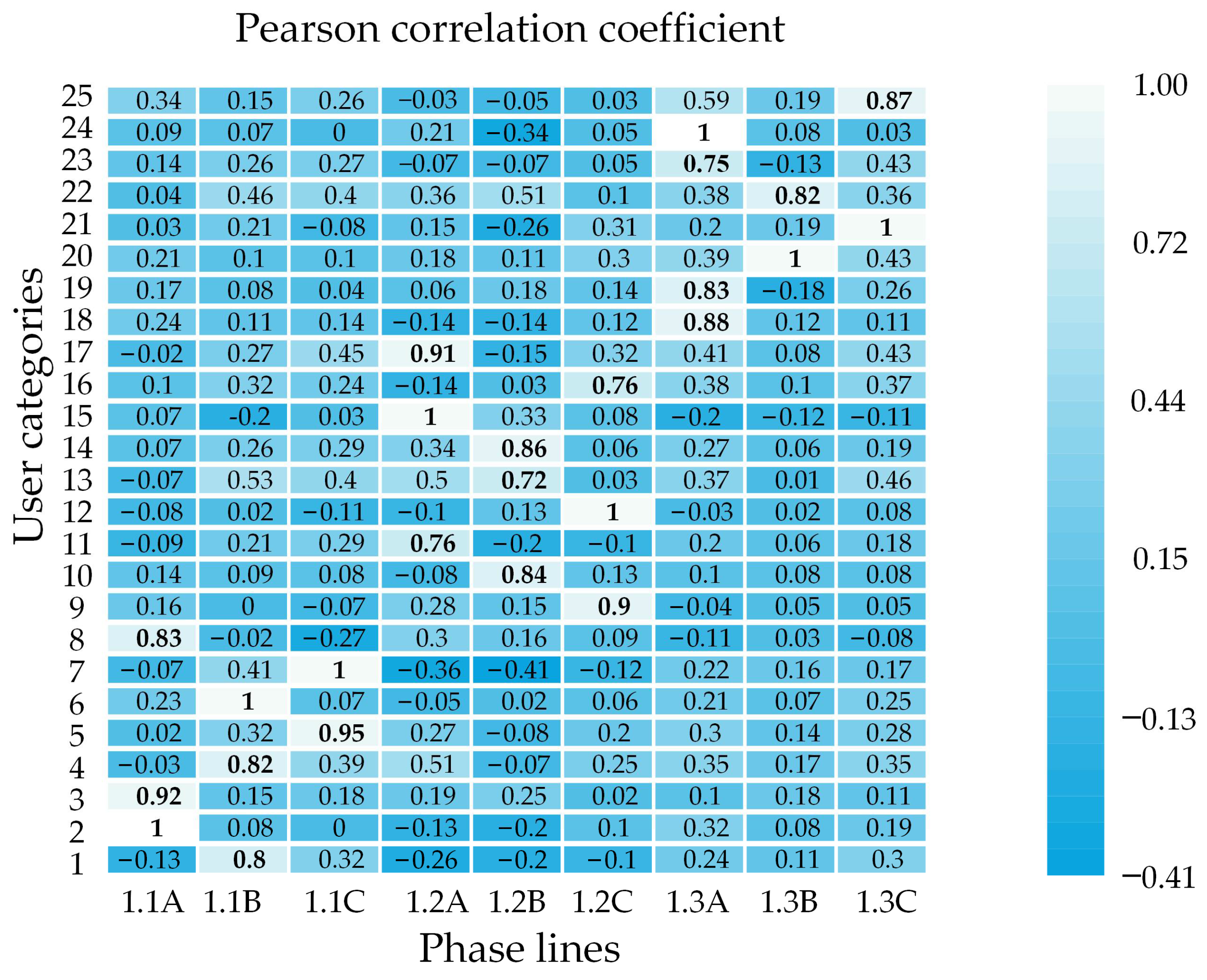
Based on the user clustering results presented in Table 1, the electricity data for the 25 categories and 9 phase lines are subjected to matrix processing. Then, following the electricity significance analysis method proposed in Section 2.4, salient feature points with significant changes in electricity consumption are extracted to form characteristic vectors. Next, the Pearson correlation coefficients between the characteristic vectors of user categories and phase lines are calculated, with the results as depicted in Figure 3, to obtain the relationships between the categories and phase lines.

To illustrate the basis for determining the line–household relationship, user category 6 is taken as an example. Its Pearson correlation coefficient with phase line 1.1B is 1, while the coefficients with other phase lines range between −0.05 and 0.35. This demonstrates that the correlation between electricity consumption characteristics for the category and its corresponding phase line is significantly higher than that with non-affiliated phase lines.

In order to evaluate the recognition accuracy of the identification algorithm in this article, an adjacency matrix $A_{25\times 9}$ is established based on the Pearson correlation coefficient matrix, and then the adjacency matrix $B_{109\times 9}$ of the connection relationship between all users and phase lines is obtained, which is compared with the adjacency matrix composed of the actual line–household relationship of the distribution network. The recognition accuracy reached 100%. The two adjacency matrices are shown in Figure A4. The identification results are displayed in

Table 2. LHRI results.

Phase Lines	Users
1.1A	U4, U5, U6, U7, U8, U9, U10, U11, U12, U30, U31, U32, U33, T1A
1.1B	U1, U2, U3, U13, U14, U15, U16, U17, U18, U24, U25, U26, T1B
1.1C	U19, U20, U21, U22, U23, U27, U28, U29, T1C
1.2A	U41, U42, U43, U44, U55, U56, U57, U63, U64, U65, U66, U67, U68
1.2B	U38, U39, U40, U48, U49, U50, U51, U52, U53, U54
1.2C	U34, U35, U36, U37, U45, U46, U47, U58, U59, U60, U61, U62
1.3A	U69, U70, U71, U72, U73, U74, U75, U76, U77, U78, U96, U97, U98, U99, U100, T2A, T3A
1.3B	U79, U80, U81, U82, U83, U84, U85, U90, U91, U92, U93, U94, U95, T2B, T3B
1.3C	U86, U87, U88, U89, T2C, T3C

.

4.4. Comparison Analysis with Other Published Methods

In existing low-voltage station area topology-identification methods, carrier waveform communication technology is usually used to identify the line-to-household relationship, and the comparison with data analysis methods tends to be complicated. The method described in this article can still accurately identify line–household relationships when the error is 0.2%. The advantages of the method are further highlighted by comparing the performance of different methods in identifying the line–household relationship. We compared this method with the Pearson correlation coefficient (Method 1) and gray correlation analysis (Method 2). The Pearson correlation coefficient is based on the correlation of electricity consumption changes, analyzing the correlation between the station line and user electricity consumption changes to identify the line–household ownership relationship; gray correlation analysis is based on the similarity of the voltage curve. Through the voltage time-series curve, the closeness of the relative change trend is used to judge the ownership relationship of lines and households in LVDNs. The results are shown in

Table 3. Identification accuracy of different methods.

Methods	LHRI Accuracy/%
	0.05%	0.1%	0.2%
Method 1	87.0	82.4	71.4
Method 2	93.3	87.5	80.7
Proposed method	100.0	100.0	100.0

.

It can be seen from Table 3 that the accuracy of Method 1 decreases as the error increases, and the error resistance is weak. Vacant users are difficult to identify because their power consumption characteristics are not obvious. Method 2 can easily lead to the misjudgment of topological information of vacant users. This causes the problem of low accuracy in identifying line–household relationships; the method in this paper has better stability against error noise. Through user voltage clustering, it associates vacant users with ordinary users and combines electricity consumption characteristics to solve the problem of identifying vacant users. It also increased the line user recognition rate to 100%. Comparative analysis verifies that the method proposed in this article has certain advantages in LHRI.

4.5. Impact Analysis of Measurement Error and Data Length

The analysis of measurement data focuses on the tolerance of uncertainty and errors. To study the impact of measurement errors and data length on the identification results, tests are conducted on 7-day, 10-day, and 15-day measurement data with added Gaussian noise. The Gaussian noise has a mean of zero and variable standard deviations. Each error distribution scenario is set to 100 iterations. For each scenario, the accuracy rates are averaged, and this average value is then used as the identification accuracy of the proposed method under that particular Gaussian error. The identification results are depicted in Figure 4.

As seen in Figure 4, when the measurement error of low-voltage district data is within 0.2%, the identification accuracy for the line–household relationship is 100%. As the measurement error exceeds 0.2%, the accuracy of identification begins to decline. The accuracy of identification demonstrates an upward trend with the increase in sample volume, indicating that identification accuracy improves with the extension of data length. Even when the measurement error reaches 0.5%, the identification correctness based on three classes of data samples remains above 94%. Nowadays, the error accuracy trend is getting higher and higher, with most accuracy rates being 0.2% or 0.5%. Within the error range of the above study, the method proposed in this article can accurately identify line–household relationships and has good results. When the error is greater than 0.5%, the discrepancy between measured and actual voltage magnitudes becomes significant due to the voltage magnitude having a large base value. This leads to vacant users and ordinary users with the closest electrical relationship not being associated due to insufficiently distinguishable voltage–time curve similarities, thus hampering the subsequent identification of line–household relationships, or mistakenly classifying users into other categories, affecting the accuracy of the proposed method. However, with the increase in data length, the aforementioned misjudgment situation will gradually improve.

5. Conclusions

To accurately obtain the line–household connection relationship in low-voltage areas, a method for LHRI based on voltage clustering and electricity consumption temporal feature analysis was proposed, leading to the following conclusions:

(1)

The clustering of customers based on the correlation of voltage time-series curves enables the linking of topological information between vacant users and regular users. This effectively addresses the issue of LHRI for vacant users and can also reduce the number of variables in the line–household identification model.

(2)

By analyzing the characteristics of electricity consumption changes between users and phase lines over long time periods and examining the correlation of their feature vectors, the connections between lines and users can be accurately determined.

(3)

The proposed method demonstrates greater stability when dealing with errors and anomalies in electrical data under different measurement environments, and the larger the length of the electrical data, the higher the accuracy of the LHRI.

In the practical engineering application environment, a multitude of uncertain factors present challenges to the performance of algorithms. Firstly, the actual measurement errors of electricity meters may not fully conform to predefined standards. Additionally, extrinsic variables such as illegal electricity theft, subpar data acquisition communication quality, measurement errors among different meters, and issues with meter synchronization all have the potential to cause significant discrepancies between collected data and the data expected under ideal conditions. In light of this, future research will be dedicated to a more in-depth analysis of these influencing factors and the exploration of methods to enhance the adaptability of the algorithm. Through these efforts, we hope to bolster the algorithm’s ability to adapt to real-world application environments and to better meet the practical demands of engineering projects.