Effect of Displacement Pressure Gradient on Oil–Water Relative Permeability: Experiment, Correction Method, and Numerical Simulation

Abstract

Relative permeability is a fundamental parameter affecting reservoir development performance analysis. During the development of oil and gas fields, the displacement pressure gradient changes with time and space. This paper studies the effect of displacement pressure gradient on relative permeability. The oil–water relative permeability curves of a Bohai Oilfield under different displacement pressure gradients are obtained through experimental analysis. Based on the experimental data, a correction model of the permeability curve is established by regression of the Willhite model parameters. The correction model is introduced into the black oil numerical simulation, and the production performance and remaining oil are compared and analyzed. The results show that the displacement pressure gradient can have an obvious impact on the relative permeability curve. As the displacement pressure gradient increases, the two-phase span of the relative permeability curve increases, the oil displacement efficiency increases, and the water relative permeability increases. The relative permeability curves under different displacement pressure gradients can be accurately characterized by the Willhite model. The consideration of the displacement pressure gradient has an obvious impact on numerical simulation results. The conventional method of using a fixed relative permeability curve cannot truly reflect the production performance and the remaining oil distribution. This paper proposes a set of realization methods including obtaining laws from experiments, utilizing the empirical model to correct, and simulating to characterize reservoir changes.

1. Introduction

Two-phase or multiphase flow in oil and gas reservoirs is a very complex process. Relative permeability is adopted to characterize the seepage law of each phase at different saturations, which is a key parameter affecting the prediction of well-production dynamics and the distribution of the remaining oil and gas [1,2,3,4].

The measurement of relative permeability for oil–water two-phase flow encompasses laboratory core tests, numerical simulation, and field tests. A core test in the lab relies on actual samples to ascertain the permeability of fluids at diverse saturation levels, while numerical simulations use computational models to mimic the porous structure of rocks and fluid movement to estimate permeability. Field tests apply targeted downhole methods to derive permeability data from oilfields. The method selection is informed by the specific context, desired precision, and resources at hand. Core tests, which include steady-state and unsteady-state methods, are essential for assessing reserves and development strategies. The steady-state method ensures stable results through a constant fluid flow in core samples, although it is time consuming. In contrast, the unsteady-state method is quicker but requires intricate data interpretation, often using the JBN method (Johnson–Bossler–Naumann Method). The JBN method analyzes pressure changes and fluid production through the Buckley–Leverett equation to calculate core relative permeability [5].

In the realm of reservoir engineering, the typical presentation of experimental data detailing the relative permeability of oil and water phases is through segmented tables. However, this format does not meet the industry’s need for a more continuous stream of data that delineates the relationship between interfacial permeability and water saturation, which is more pragmatically expressed through mathematical formulations. This gap has prompted researchers globally to engage in extensive regression analyses, leveraging the robust datasets of oil–water relative permeability. These endeavors have culminated in a plethora of mathematical models that articulate the dynamic oil–water flow process [6,7,8]. Significantly, these models encapsulate the nuances of the displacement phenomenon observed during the genesis of reservoirs as well as the imbibition phenomenon pertinent to the developmental phase of oilfields. Imbibition models, for their part, are extensively utilized in the operational sphere of oilfield management. Among the various models, the Willhite model is frequently utilized in the field due to its ability to effectively address the issue of zero relative permeability at both residual oil and bound water endpoints [9]. The model’s strengths lie in its responsiveness to the relative permeability characteristics of oil and water phases, which are predominantly influenced by the exponents of oil and water phases. This feature is particularly advantageous for swiftly comparing permeability variations across different reservoirs or storage layers, offering convenience in rapid analysis.

According to traditional research, relative permeability is an inherent property of porous media. It is affected by the physical properties of rocks and fluids. These physical parameters include pore structure, wettability, interfacial tension, fluid viscosity, stress, and temperature. Pore structure impacts the capillary pressures and, thus, the saturation levels at which oil and water will flow [10,11,12]. The wettability affects how oil and water distribute within the pore space, determining which fluid is more easily displaced [13,14,15]. Higher interfacial tension can increase capillary forces, trapping fluids and altering their flow, while lower interfacial tension can enhance displacement of one fluid by another [16,17,18,19]. Fluid viscosity influences the mobility ratio between oil and water, affecting the sweep efficiency during recovery [20,21,22]. Changes in the overburden or pore pressure can alter pore structure and fluid distribution, impacting relative permeability [23,24,25,26]. Temperature affects fluid viscosity and interfacial tension, thus influencing fluid flow and relative permeability in the reservoir [27,28,29,30,31,32].

Additionally, many scholars have studied the impact of reservoir development dynamic parameters, including waterflooding pore volume [31,32,33], displacement pressure gradient [34,35], and flow velocity [21,36,37,38]. Unlike the static parameters, there is no generally accepted understanding of the effects of dynamic parameters on relative permeability, especially displacement pressure gradient and flow velocity. Although the flow rate dependency of relative permeability has been observed since the earliest core flooding experiments [38], whether displacement pressure gradient and flow rate impact relative permeability has been controversial. Ehrlich et al. [39] concluded that relative permeability at a given saturation is everywhere independent of flow rate. Botset [40] showed that the dependency of relative permeability on flow rate is related to the end effect of the core. However, with the application of CT scanning technology, the development of network models, and the improvement of experimental accuracy, most of the research results in recent years have pointed out the impact of displacement pressure gradient and flow rate on relative permeability. Krause et al. [36] demonstrated the flow rate dependency of relative permeability through numerical simulations of steady-state core flooding experiments conducted at several injection rates. Liu et al. [34] carried out the oil–water relative permeability experiments with three different displacement pressures on the same extra-low-permeability core using the unsteady experimental method. The result shows that as the displacement pressure enlarges, the relative permeabilities of oil and water both increase; the residual oil saturation decreases and the range of the two-phase flow zone is improved. Keshavarz et al. [35] conducted an experimental investigation of the effect of pressure gradient on gas–oil relative permeability in Iranian carbonate rocks. Results show that relative permeability curves are affected by pressure gradient and this effect is much more prominent at low pressures due to end-effect phenomena. The dependence of relative permeability curves on pressure gradient is correlated as a function of dimensionless capillary number. Nguyen et al. [41] established a dynamic network model to study the effect of displacement rate on imbibition relative permeability and residual saturation. It was concluded that increasing the rate results in more favorable relative permeability curves and lower residual saturations. Rabinovich [42] found that the relative permeability curves may change at lower rates through core flooding experiments, as capillary heterogeneity effects become significant.

From the above research results, it can be seen that the physical simulation of the impact of the displacement pressure gradient or the flow velocity on relative permeability is relatively mature. However, the dynamic change of relative permeability significantly influences the reservoir development law. It is necessary to apply the change of the relative permeability curve to the prediction of development performance. In the traditional numerical simulation, the relative permeability curve is fixed throughout the entire development mileage. Therefore, the relative permeability curves of cores from Bohai Oilfield under different displacement pressure gradients were taken as the basis for research. A correction method was established with parameter regression of the Willhite model, a mature mathematical model of relative permeability. The correction model was then introduced into the numerical simulation by modifying codes of the open-source reservoir numerical simulation tool MRST (MATLAB Reservoir Simulation Toolbox 2022b). A research process from core analysis to field simulation is performed.

2. Experimental Analysis

The unsteady displacement state method is used to measure the oil–water relative permeability under different displacement pressure gradients. The experimental apparatus is shown in Figure 1, which includes the fluid injection part, core model, confining pressure control part, temperature control part, pressure detection part, and outlet metering part.

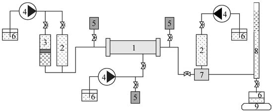
Figure 1. Schematic diagram of the experimental apparatus of the relative permeability measurement. 1—Core gripper; 2—Water container; 3—Piston container; 4—Constant pressure pump; 5—Pressure sensor; 6—Beaker; 7—Back pressure valve; 8—Oil–water measuring container; 9—Electronic balance.

The study adopts reservoir parameters and sealed core samples extracted from the producing zone in a stratigraphic well at the Bohai Oilfield, China. The type of rock is sandstone. The core size is cylindrical with a diameter of 2.5 cm and a length of 5.5 cm. The physical parameters and experiment conditions of each core are shown in Table 1. It can be seen that the physical parameters are similar. The experimental temperature is 60 °C. The injected water is a potassium chloride solution with a salinity of 4862 mg/L. The viscosity of the oil is 55.00 mPa·s. The displacement pressure gradient is controlled by fixing the pressure difference at the inlet end and outlet end of the core, which, of each group of cores, is set as 0.030 MPa/m, 0.100 MPa/m, 0.300 MPa/m, and 1.500 MPa/m.

Table 1. Physical parameters of the sandstone cores and experiment conditions.

No.	Sampling Depth (m)	Porosity (%)	Permeability (mD)	Displacement Pressure Gradient (MPa/m)
1	1630.50	36.5	1255.4	0.030
2	1630.51	37.0	1319.3	0.100
3	1630.53	36.6	1293.4	0.300
4	1630.54	36.8	1313.1	0.700
5	1630.55	36.6	1344.8	1.500

The experimental process is carried out under constant pressure difference according to the Chinese national standard [43]. Specific steps are as follows:

(1)

The cores are vacuumed and saturated with formation water after being washed and dried.

(2)

The cores are put into the gripper for oil flooding. Establish initial irreducible water saturation by flooding until no water flows out. The effective permeability of the oil phase under irreducible water saturation is measured.

(3)

The oil is displaced by formation water under the selected displacement pressure difference. The water breakthrough time, cumulative oil production, cumulative liquid production, and pressure at both ends of the core holder are recorded accurately.

(4)

Use the JBN method to process data and output the relative permeability curves.

The relative permeability curves of each group of cores obtained from the experiment are shown in Figure 2, and the saturation and relative permeability values at the endpoint of each curve are shown in Table 2. It can be seen that due to the close location and similar physical properties of the core samples, the difference in irreducible water saturation of each phase permeability curve is very small, which can be ignored.

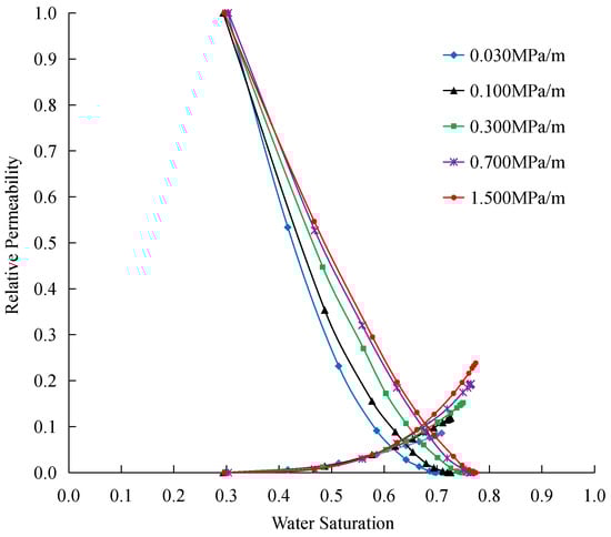
Figure 2. Experiment results of oil–water relative permeability under different displacement pressure gradients.

Table 2. Endpoint parameters of each oil–water permeability curve.

No.	Displacement Pressure Gradient (MPa/m)	Irreducible Water Saturation	Residual Oil Saturation	Maximum Water Relative Permeability	Oil Displacement Efficiency
1	0.030	0.3021	0.2908	0.0859	0.5833
2	0.100	0.2937	0.2735	0.1194	0.6128
3	0.300	0.2969	0.2498	0.1523	0.6447
4	0.700	0.3035	0.2321	0.1937	0.6668
5	1.500	0.2956	0.2259	0.2388	0.6793

Under different displacement pressure gradients, the displacement efficiency and curve shape show obvious differences. The two-phase span increases with the displacement pressure gradient, representing an improvement in oil displacement efficiency. Quantitatively, the change of the oil–water relative permeability curve is reflected in three parts: the change of residual oil saturation, maximum water relative permeability, and curve camber. With the increase in the displacement pressure gradient, the residual oil saturation decreases, the maximum water relative permeability increases, the camber of the water phase curve increases, and the camber of the oil phase curve decreases. Therefore, this paper corrects the relative permeability curve by characterizing the variation of these three parameters.

3. Correction Method

It is vital to select an appropriate mathematical model to describe the effects of displacement pressure gradient on the relative permeability curve. Scholars have put forward many mathematical models based on regression analysis of experimental data. The Willhite model is relatively mature in application among those models. Its biggest advantage is that the endpoint values can be accurately represented. The equations of the Willhite model are

$${\mathrm{K}}_{\mathrm{rw}}={\mathrm{K}}_{\mathrm{rw}}\left({\mathrm{S}}_{\mathrm{or}}\right){\mathrm{S}}_{\mathrm{wd}}^{\mathrm{m}},$$

(1)

$${\mathrm{K}}_{\mathrm{ro}}={\mathrm{K}}_{\mathrm{ro}}\left({\mathrm{S}}_{\mathrm{wc}}\right){\left(1-{\mathrm{S}}_{\mathrm{wd}}\right)}^{\mathrm{n}},$$

(2)

$${\mathrm{S}}_{\mathrm{wd}}=\frac{{\mathrm{S}}_{\mathrm{w}}-{ \mathrm{S}}_{\mathrm{wc}}}{1-{ \mathrm{S}}_{\mathrm{or}}-{ \mathrm{S}}_{\mathrm{wc}}},$$

(3)

where ${\mathrm{K}}_{\mathrm{rw}}$ is the water relative permeability, fraction; ${\mathrm{K}}_{\mathrm{rw}}\left({\mathrm{S}}_{\mathrm{or}}\right)$ is the water relative permeability under residual oil saturation (i.e., the maximum water relative permeability), fraction; ${\mathrm{K}}_{\mathrm{ro}}$ is the oil relative permeability, fraction; ${\mathrm{K}}_{\mathrm{ro}}\left({\mathrm{S}}_{\mathrm{wc}}\right)$ is the oil relative permeability under irreducible water saturation, fraction; ${\mathrm{S}}_{\mathrm{wd}}$ is normalized water saturation, fraction; ${\mathrm{S}}_{\mathrm{w}}$ is water saturation, fraction; ${\mathrm{S}}_{\mathrm{wc}}$ is irreducible water saturation, fraction; ${\mathrm{S}}_{\mathrm{or}}$ is residual oil saturation, fraction; and $\mathrm{m}$ and $\mathrm{n}$ are the coefficients of water and oil phase curves concerning camber, respectively.

In the Willhite model, the residual oil saturation and the maximum water relative permeability are the parameters of the model. The curve camber is characterized by a power law and defined by the coefficients $\mathrm{m}$ and $\mathrm{n}$. In this paper, the correction model of the relative permeability curve is established by quantifying the variation of the Willhite model coefficients $\mathrm{m}$ and $\mathrm{n}$, residual oil saturation, and maximum water relative permeability with the displacement pressure gradient.

3.1. Willhite Model Coefficients $m$ and $n$

The change of coefficients $\mathrm{m}$ and $\mathrm{n}$ can be extracted through normalization. Before analyzing the relative permeability curve with the Willhite model, the experimental data shall be normalized according to Equation (3) and the following equations:

$${\mathrm{K}}_{\mathrm{rw}}^{\prime }=\frac{{\mathrm{K}}_{\mathrm{rw}}}{{\mathrm{K}}_{\mathrm{rw}}\left({\mathrm{S}}_{\mathrm{or}}\right)},$$

(4)

$${\mathrm{K}}_{\mathrm{ro}}^{\prime }=\frac{{\mathrm{K}}_{\mathrm{ro}}}{{\mathrm{K}}_{\mathrm{ro}}\left({\mathrm{S}}_{\mathrm{wc}}\right)},$$

(5)

where ${\mathrm{K}}_{\mathrm{rw}}^{\prime }$ is the normalized water relative permeability, fraction and ${\mathrm{K}}_{\mathrm{ro}}^{\prime }$ is the normalized oil relative permeability, fraction.

The normalized oil–water relative permeability curves are shown in Figure 3. Compared with the original curves, it is more easily observed that with the increase in the displacement pressure gradient, the camber of the oil-phase curve decreases and the camber of the water-phase curve increases.

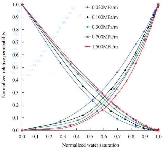
Figure 3. Normalized oil–water relative permeability curves under different displacement pressure gradients.

By combining Equations (1), (2), (4) and (5), the relationship between normalized relative permeability and normalized water saturation can be obtained:

$${\mathrm{K}}_{\mathrm{rw}}^{\prime }={\mathrm{S}}_{\mathrm{wd}}^{\mathrm{m}},$$

(6)

$${\mathrm{K}}_{\mathrm{ro}}^{\prime }={\left(1-{\mathrm{S}}_{\mathrm{wd}}\right)}^{\mathrm{n}}.$$

(7)

Based on the above equations, the normalized oil–water relative permeability curves under different displacement pressure gradients are fitted. As shown in Figure 4, high fitting accuracy has been achieved, which means the Willhite model can accurately reflect the change rule of the relative permeability curve with the displacement pressure gradient.

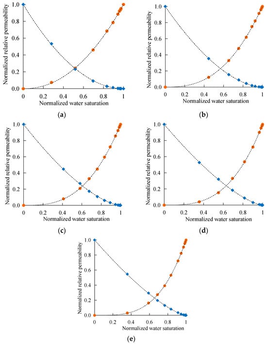
Figure 4. Fitting results of relative permeability curves under different displacement pressure gradients. (a) 0.030 MPa/m; (b) 0.100 MPa/m; (c) 0.300 MPa/m; (d) 0.700 MPa/m; (e) 1.500 MPa/m. Orange dots represent water phase; blue squares represent the oil phase.

According to the fitting results shown in Figure 3, the coefficients $\mathrm{m}$ and $\mathrm{n}$ under different displacement pressure gradients are obtained, as shown in Table 3. With the increase in the displacement pressure gradient, $\mathrm{m}$ increases and $\mathrm{n}$ decreases gradually. Figure 5 shows the regression relationship between the coefficients $\mathrm{m}$ and $\mathrm{n}$ and the displacement pressure gradient. The corresponding expression is

$$\mathrm{m}=3.2996{\mathrm{D}}^{0.1183},$$

(8)

$$\mathrm{n}=1.4036{\mathrm{D}}^{-0.0926},$$

(9)

where $\mathrm{D}$ is the displacement pressure gradient, MPa/m.

Table 3. Values of coefficients $\mathrm{m}$ and $\mathrm{n}$ under different displacement pressure gradients.

No.	Displacement Pressure Gradient (MPa/m)	m	n
1	0.030	2.1315	1.9582
2	0.100	2.6060	1.7469
3	0.300	2.8750	1.5318
4	0.700	3.0861	1.4346
5	1.500	3.4824	1.3812

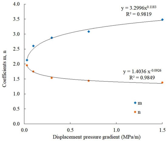
Figure 5. Coefficients $\mathrm{m}$ and $\mathrm{n}$ under different displacement pressure gradients.

The relationship satisfies the power law, and the correlation coefficient R² of the regression results is above 0.98. Correction of coefficients $\mathrm{m}$ and $\mathrm{n}$ can be obtained through Equations (8) and (9).

3.2. Residual Oil Saturation

To weaken the influence of the physical property difference of core samples on residual oil saturation, the change rule of residual oil saturation is characterized indirectly by displacement efficiency. As Figure 6 shows, the regression relationship between oil displacement efficiency and displacement pressure gradient meets the logarithmic function. The corresponding expression is

$${\mathrm{E}}_{\mathrm{D}}=2.5301\ln \mathrm{D}+67.2616,$$

(10)

where ${\mathrm{E}}_{\mathrm{D}}$ is the oil displacement efficiency, fraction.

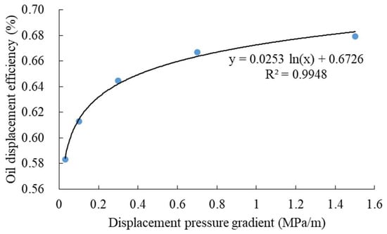
Figure 6. The displacement efficiency under different displacement pressure gradients.

According to the definition of oil displacement efficiency, residual oil saturation can be expressed as

$${\mathrm{S}}_{\mathrm{or}}=1-{\mathrm{S}}_{\mathrm{wc}}-{\mathrm{E}}_{\mathrm{D}}\left(1-{\mathrm{S}}_{\mathrm{wc}}\right),$$

(11)

Combining Equations (10) and (11), the following equation can be obtained:

$${\mathrm{S}}_{\mathrm{or}}=1-{\mathrm{S}}_{\mathrm{wc}}-\left(0.0253\ln \mathrm{D}+0.6726\right)\left(1-{\mathrm{S}}_{\mathrm{wc}}\right),$$

(12)

The irreducible water saturations of five sets of relative permeability curves are the same. Therefore, an average value is taken as 0.2984. Then, the residual oil saturation under different displacement pressure gradients can be calculated from the following equation:

$${\mathrm{S}}_{\mathrm{or}}=-0.0178\ln \mathrm{D}+0.2297,$$

(13)

3.3. Maximum Water Relative Permeability

According to the experimental data in Table 2, the regression relationship between the maximum water relative permeability and the displacement pressure gradient is established, as shown in Figure 7. The equation obtained is

$${\mathrm{K}}_{\mathrm{rw}}\left({\mathrm{S}}_{\mathrm{or}}\right)=0.2128{\mathrm{D}}^{0.2583}.$$

(14)

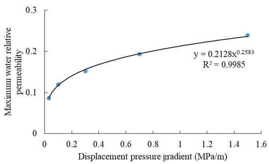
Figure 7. The maximum water relative permeability under different displacement pressure gradients.

3.4. Correction Steps

Through Equations (8), (9), (13), and (14), the Willhite model coefficients $\mathrm{m}$ and $\mathrm{n}$, residual oil saturation, and maximum water relative permeability can be corrected for displacement pressure gradient. In a specific application, the displacement pressure gradient is determined first, and then, the relative permeability curve is calculated according to the following steps:

(a)

Calculate residual oil saturation ${\mathrm{S}}_{\mathrm{or}}$ using Equation (13);

(b)

Calculate the maximum water relative permeability ${\mathrm{K}}_{\mathrm{rw}}\left({\mathrm{S}}_{\mathrm{or}}\right)$ using Equation (14);

(c)

Calculate the Willhite model coefficients $\mathrm{m}$ and $\mathrm{n}$ using Equations (8) and (9), respectively;

(d)

The oil–water relative permeability curve is calculated using Equations (1)–(3).

4. Application in Numerical Simulation

The current common commercial reservoir numerical simulation software (Intersect 2023, Eclipse 2023, CMG 2022, tNavigator 2022, etc.) does not have the function or module to characterize the change of the relative permeability curve with displacement pressure gradient. In this paper, the open-source reservoir numerical simulation tool MRST (MATLAB Reservoir Simulation Toolbox) is used to implement the relative permeability curve changing with the displacement pressure gradient. This tool provides black oil and component simulators and is widely used in the research of oil and gas reservoir seepage mechanisms and new understandings [44]. In the source code of the black oil simulator, the oil–water relative permeability curve correction module is embedded according to the steps in Section 3.4, and the simulation flow chart is shown in Figure 8.

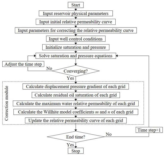
Figure 8. Flowchart of numerical simulation of black oil embedded in oil–water permeability curve correction.

To analyze the effect of the displacement pressure gradient on production performance and remaining oil distribution, a five-point well pattern conceptual model is established as shown in Figure 9. In the numerical simulation of waterflooding reservoirs, the choice of grid size usually takes into account the impact of the number of grids on the calculation speed and whether the changes in saturation and pressure fields between oil and water wells can be accurately determined. The horizontal grid size is generally between 5 and 50m, and the longitudinal grid size is generally between 1 and 5 m. In this study, the number of model grids is 41 × 41 × 5. The horizontal dimension of the grids is 10 m and the vertical dimension is 2 m. The porosity is 36.7%. The horizontal permeability is 2000 mD and the vertical permeability is 130 mD. The formation oil viscosity is 55.0 mPa·s and the oil volume coefficient is 1.065. The initial relative permeability curve is set using the data of 0.100 MPa/m in Figure 2. The production wells are controlled with a constant liquid rate of 120 m³/d. The injection well is controlled by an injection–production ratio of 1.0.

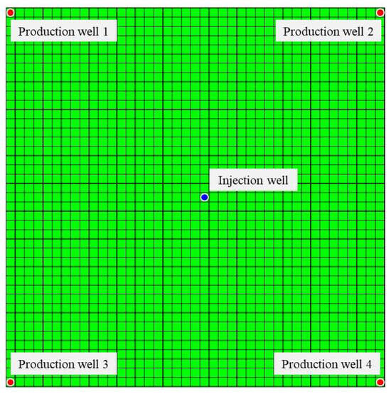
Figure 9. The grid layout and well pattern of the conceptual model.

The simulation results with and without the effect of displacement pressure gradient on relative permeability were compared. In the simulation without the effects of displacement pressure gradient, only the initial relative permeability curve was adopted. The difference in the production water cut is shown in Figure 10. When the effect of the displacement pressure gradient is considered, the oil production period without water is prolonged from 195 days to 285 days. The water cut in the early stage of reservoir production is lower with the effect of the displacement pressure gradient, which is reduced from 55.8% to 51.9% on the 1000th day. This is due to the higher pressure gradient in the near-wellbore area, which increases the displacement efficiency. However, the water cut is higher in the later stages. This is the result of higher water relative permeability and rapid water breakthrough in areas with high displacement degrees. The water cut is increased from 94.7% to 95.9% on the 6000th day with the effect of the displacement pressure gradient. In this conceptual model, the factor that the displacement pressure gradient improves the displacement efficiency plays a major role. This results in a higher recovery degree when the effect of displacement pressure gradients is considered, which is increased from 41.0% to 42.6% on the 6000th day as shown in Figure 11.

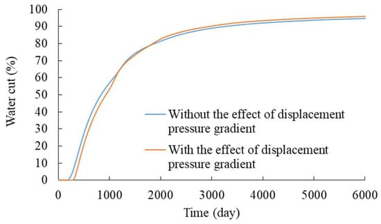
Figure 10. Comparison of water cut with and without the effect of displacement pressure gradient.

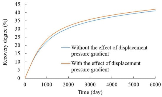
Figure 11. Comparison of recovery factor with and without the effect of displacement pressure gradient.

The comparison of the remaining oil saturation in the third layer grid when the water cut is 20%, 60%, and 90% is shown in Figure 12, Figure 13 and Figure 14. When considering the effect of displacement pressure gradient, due to the large pressure gradient in the near-wellbore area and the injection–production main line, the oil displacement efficiency increases after phase permeability correction and the remaining oil saturation is lower. However, the displacement pressure gradient in the area between production wells is small, and the remaining oil saturation is higher. The remaining oil saturation profile between injection and production wells is compared in Figure 15, Figure 16 and Figure 17. Due to the density stratification between the water and oil, more oil is enriched at the top of the reservoir and more water at the bottom. When considering the effect of displacement pressure gradient, the remaining oil saturation near the injection well in all layers decreases. Differently, the saturation at the bottom near production wells is reduced, while the remaining oil is more abundant in the upper part.

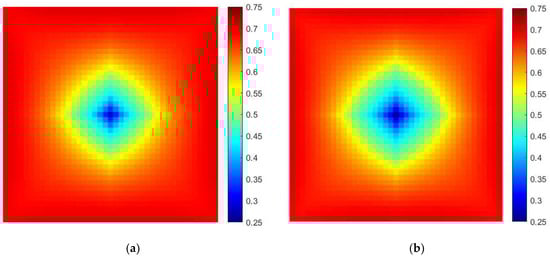
Figure 12. Comparison of the remaining oil saturation in the third layer grid when the water cut is 20%. (a) Without the effect of displacement pressure gradient; (b) with the effect of displacement pressure gradient.

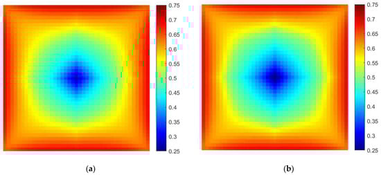
Figure 13. Comparison of the remaining oil saturation in the third layer grid when the water cut is 60%. (a) Without the effect of displacement pressure gradient; (b) with the effect of displacement pressure gradient.

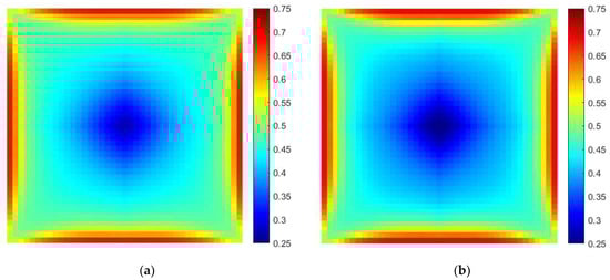
Figure 14. Comparison of the remaining oil saturation in the third layer grid when the water cut is 90%. (a) Without the effect of displacement pressure gradient; (b) with the effect of displacement pressure gradient.

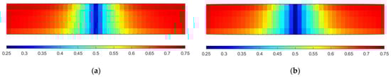
Figure 15. Comparison of remaining oil saturation profiles between injection and production wells when the water cut is 20%. (a) Without the effect of displacement pressure gradient; (b) with the effect of displacement pressure gradient.

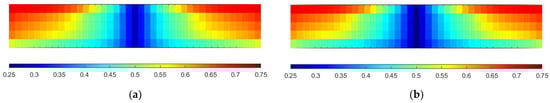
Figure 16. Comparison of remaining oil saturation profiles between injection and production wells when the water cut is 60%. (a) Without the effect of displacement pressure gradient; (b) with the effect of displacement pressure gradient.

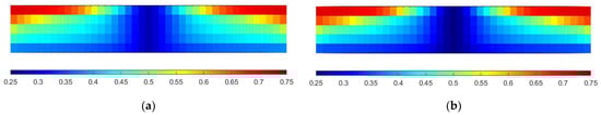
Figure 17. Comparison of remaining oil saturation profiles between injection and production wells when the water cut is 90%. (a) Without the effect of displacement pressure gradient; (b) with the effect of displacement pressure gradient.

5. Conclusions

In this paper, the effect of the displacement pressure gradient on relative permeability is studied through experiment, correction model, and numerical simulation. The following main conclusions were drawn:

(1)

The displacement pressure gradient can have an obvious impact on the relative permeability curve. For the cores from Bohai Oilfield tested in this paper, as the displacement pressure gradient increases, the two-phase span of the relative permeability curve increases, the oil displacement efficiency increases, and the relative water permeability increases.

(2)

The relative permeability curves under different displacement pressure gradients can be characterized by the Willhite model. The variation of model parameters has good regression. The relative permeability curves can be obtained by correcting the parameters of the Willhite model.

(3)

Considering the effect of the displacement pressure gradient on relative permeability will have an obvious impact on numerical simulation results. The conventional method of using a fixed relative permeability curve cannot truly reflect the production performance of the reservoir. The distribution of the remaining oil is also obviously different.

(4)

This paper proposes a set of realization methods including obtaining laws from experiments, utilizing the empirical model to correct, and simulating to characterize reservoir changes. It can provide a reference for those who research the effect of the displacement pressure gradient on relative permeability.

References

- Salmachi, A.; Karacan, C.Ö. Cross-Formational Flow of Water into Coalbed Methane Reservoirs: Controls on Relative Permeability Curve Shape and Production Profile. Environ. Earth Sci. 2017, 76, 200. [Google Scholar] [CrossRef]
- Lian, P.; Cheng, L.; Liu, L. The Relative Permeability Curve of Fractured Carbonate Reservoirs. Shiyou Xuebao/Acta Pet. Sin. 2011, 32, 1026–1030. [Google Scholar]
- Kadkhodaie, A.; Rezaee, R.; Kadkhodaie, R. An Effective Approach to Generate Drainage Representative Capillary Pressure and Relative Permeability Curves in the Framework of Reservoir Electrofacies. J. Pet. Sci. Eng. 2019, 176, 1082–1094. [Google Scholar] [CrossRef]
- Pini, R.; Benson, S.M. Simultaneous Determination of Capillary Pressure and Relative Permeability Curves from Core-Flooding Experiments with Various Fluid Pairs. Water Resour. Res. 2013, 49, 3516–3530. [Google Scholar] [CrossRef]
- Johnson, E.F.; Bossler, D.P.; Bossler, V.O.N. Calculation of Relative Permeability from Displacement Experiments. Trans. AIME 1959, 216, 370–372. [Google Scholar] [CrossRef]
- Li, K. More General Capillary Pressure and Relative Permeability Models from Fractal Geometry. J. Contam. Hydrol. 2010, 111, 13–24. [Google Scholar] [CrossRef] [PubMed]
- Moghadasi, L.; Guadagnini, A.; Inzoli, F.; Bartosek, M. Interpretation of Two-Phase Relative Permeability Curves through Multiple Formulations and Model Quality Criteria. J. Pet. Sci. Eng. 2015, 135, 738–749. [Google Scholar] [CrossRef]
- Lashgari, H.R.; Pope, G.A.; Tagavifar, M.; Luo, H.; Sepehrnoori, K.; Li, Z.; Delshad, M. A New Relative Permeability Model for Chemical Flooding Simulators. J. Pet. Sci. Eng. 2018, 171, 1466–1474. [Google Scholar] [CrossRef]
- Willhite, G.P. Waterflooding; Society of Petroleum Engineers: Richardson, TX, USA, 1986; ISBN 978-1-55563-005-8. [Google Scholar]
- Dana, E.; Skoczylas, F. Gas Relative Permeability and Pore Structure of Sandstones. Int. J. Rock Mech. Min. Sci. 1999, 36, 613–625. [Google Scholar] [CrossRef]
- Wang, L.J.; Bai-Ling, F.U. Analysis of Oil-Water Relative Permeability Curve’s Characteristics. Sci. Technol. Eng. 2012, 12, 2160–2162. [Google Scholar]
- Kanellopoulos, N.K.; Petropoulos, J.H.; Nicholson, D. Effect of Pore Structure and Macroscopic Non-Homogeneity on the Relative Gas Permeability of Porous Solids. J. Chem. Soc. Faraday Trans. 1 Phys. Chem. Condens. Phases 1985, 81, 1183–1194. [Google Scholar] [CrossRef]
- Dicarlo, D.A.; Sahni, A.; Blunt, M.J. The Effect of Wettability on Three-Phase Relative Permeability. Transp. Porous Media 2000, 39, 347–366. [Google Scholar] [CrossRef]
- Spiteri, E.J.; Juanes, R.; Blunt, M.J.; Orr, F.M. A New Model of Trapping and Relative Permeability Hysteresis for All Wettability Characteristics. SPE J. 2008, 13, 277–288. [Google Scholar] [CrossRef]
- Gharbi, O.; Blunt, M.J. The Impact of Wettability and Connectivity on Relative Permeability in Carbonates: A Pore Network Modeling Analysis. Water Resour. Res. 2012, 48, W12513.1–W12513.14. [Google Scholar] [CrossRef]
- Cinar, Y.; Marquez, S.; Orr, F.M. Effect of IFT Variation and Wettability on Three-Phase Relative Permeability. SPE Reserv. Eval. Eng. 2007, 10, 211–220. [Google Scholar] [CrossRef]
- Fatemi, S.M.; Sohrabi, M.; Jamiolahmady, M.; Ireland, S. Experimental and Theoretical Investigation of Gas/Oil Relative Permeability Hysteresis under Low Oil/Gas Interfacial Tension and Mixed-Wet Conditions. Energy Fuels 2012, 26, 4366–4382. [Google Scholar] [CrossRef]
- Shen, P.; Zhu, B.; Li, X.B.; Wu, Y.S. An Experimental Study of the Influence of Interfacial Tension on Water-Oil Two-Phase Relative Permeability. Transp. Porous Media 2010, 85, 505–520. [Google Scholar] [CrossRef]
- Wang, Y.S.; Yang, Y.F.; Wang, K.; Tao, L.; Liu, J.; Wang, C.C.; Yao, J.; Zhang, K.; Song, W.H. Changes in relative permeability curves for natural gas hydrate decomposition due to particle migration. J. Nat. Gas Sci. Eng. 2020, 84, 103634. [Google Scholar] [CrossRef]
- Wang, S.L.; Li, A.F.; Peng, R.G.; Miao, Y.U.; Shi, F.S.; Fang, M.Y. Effect of Oil Water Viscosity Ratio on Heavy Oil-Water Relative Permeability Curve. Sci. Technol. Eng. 2017, 17, 86–90. [Google Scholar]
- Jeong, G.S.; Lee, J.; Ki, S.; Huh, D.G.; Park, C.H. Effects of Viscosity Ratio, Interfacial Tension and Flow Rate on Hysteric Relative Permeability of CO2/Brine Systems. Energy 2017, 133, 62–69. [Google Scholar] [CrossRef]
- Esmaeili, S.; Modaresghazani, J.; Sarma, H.; Harding, T.; Maini, B. Effect of Temperature on Relative Permeability–Role of Viscosity Ratio. Fuel 2020, 278, 118318. [Google Scholar] [CrossRef]
- Alexis, D.A.; Karpyn, Z.T.; Ertekin, T.; Crandall, D. Fracture Permeability and Relative Permeability of Coal and Their Dependence on Stress Conditions. J. Unconv. Oil Gas Resour. 2015, 10, 1–10. [Google Scholar] [CrossRef]
- Al-Quraishi, A.; Khairy, M. Pore Pressure versus Confining Pressure and Their Effect on Oil-Water Relative Permeability Curves. J. Pet. Sci. Eng. 2005, 48, 120–126. [Google Scholar] [CrossRef]
- Yan, J.; Zheng, R.; Chen, P.; Wang, S.; Shi, Y. Calculation Model of Relative Permeability in Tight Sandstone Gas Reservoir with Stress Sensitivity. Geofluids 2021, 2021, 6260663. [Google Scholar] [CrossRef]
- Adenutsi, C.D.; Li, Z.; Xu, Z.; Sun, L. Influence of Net Confining Stress on NMR T2 Distribution and Two-Phase Relative Permeability. J. Pet. Sci. Eng. 2019, 178, 766–777. [Google Scholar] [CrossRef]
- Mahmud, W.M. Impact of Salinity and Temperature Variations on Relative Permeability and Residual Oil Saturation in Neutral-Wet Sandstone. Capillarity 2022, 5, 23–31. [Google Scholar] [CrossRef]
- Chen, X.; Gao, S.; Kianinejad, A.; Di Carlo, D.A. Steady-State Supercritical CO2 and Brine Relative Permeability in Berea Sandstone at Different Temperature and Pressure Conditions. Water Resour. Res. 2017, 53, 6312–6321. [Google Scholar] [CrossRef]
- Yang, L.; Shen, D.; Wang, X.; Li, Z. The Effect of Temperature on the Relative Permeability and Residual Oil Saturation. Pet. Explor. Dev. 2003, 30, 97–99. [Google Scholar]
- Balogun, Y.; Iyi, D.; Faisal, N.; Oyeneyin, B.; Oluyemi, G.; Mahon, R. Experimental Investigation of the Effect of Temperature on Two-Phase Oil-Water Relative Permeability. J. Pet. Sci. Eng. 2021, 203, 108645. [Google Scholar] [CrossRef]
- Ji, S.; Tian, C.; Shi, C.; Ye, J.; Zhang, Z.; Fu, X. New Understanding on Water-Oil Displacement Efficiency in a High Water-Cut Stage. Pet. Explor. Dev. 2012, 39, 362–370. [Google Scholar] [CrossRef]
- Feng, G.; Yu, M. Le Characterization of Pore Volume of Cumulative Water Injection Distribution. Petroleum 2015, 1, 158–163. [Google Scholar] [CrossRef]
- Qi, G.; Zhao, J.; He, H.; Sun, E.; Yuan, X.; Wang, S. A New Relative Permeability Characterization Method Considering High Waterflooding Pore Volume. Energies 2022, 15, 3868. [Google Scholar] [CrossRef]
- Liu, Q.; Wu, K.; Li, X.; Tu, B.; Zhao, W.; He, M.; Zhang, Q.; Xie, Y. Effect of Displacement Pressure on Oil-Water Relative Permeability for Extra-Low-Permeability Reservoirs. ACS Omega 2021, 6, 2749–2758. [Google Scholar] [CrossRef]
- Keshavarz, A.; Vatanparast, H.; Zargar, M.; Asl, A.K.; Haghighi, M. An Experimental Investigation of the Effect of Pressure Gradient on Gas-Oil Relative Permeability in Iranian Carbonate Rocks. Pet. Sci. Technol. 2012, 30, 1508–1522. [Google Scholar] [CrossRef]
- Krause, M.H.; Benson, S.M. Accurate Determination of Characteristic Relative Permeability Curves. Adv. Water Resour. 2015, 83, 376–388. [Google Scholar] [CrossRef]
- Herderson, G.D.; Danesh, A.; Tehrani, D.H. Effect of Positive Rate Sensitivity and Inertia on Gas Condensate Relative Permeability at High Velocity. Pet. Geosci. 2001, 7, 45–50. [Google Scholar] [CrossRef]
- Leverett, M.C. Flow of Oil-Water Mixtures through Unconsolidated Sands. Trans. AIME 1939, 132, 149–171. [Google Scholar] [CrossRef]
- Ehrlich, R.; Crane, F.E. A Model for Two-Phase Flow in Consolidated Materials. Soc. Pet. Eng. J. 1969, 9, 221–231. [Google Scholar] [CrossRef]
- Botset, H.G. Flow of Gas-Liquid Mixtures through Consolidated Sand. Trans. AIME 1940, 136, 91–105. [Google Scholar] [CrossRef]
- Nguyen, V.H.; Sheppard, A.P.; Knackstedt, M.A.; Val Pinczewski, W. The Effect of Displacement Rate on Imbibition Relative Permeability and Residual Saturation. J. Pet. Sci. Eng. 2006, 52, 54–70. [Google Scholar] [CrossRef]
- Rabinovich, A. Analytical Corrections to Core Relative Permeability for Low-Flow-Rate Simulation. SPE J. 2018, 23, 1851–1865. [Google Scholar] [CrossRef]
- GB/T 28912-2012; Test Method for Two Phase Relative Permeability in Rock. National Petroleum Standardization Technical Committee: Beijing, China, 2012.
- Lie, K.A. An Introduction to Reservoir Simulation Using MATLAB/GNU Octave: User Guide for the MATLAB Reservoir Simulation Toolbox (MRST); Cambridge University Press: Cambridge, UK, 2019; Available online: https://www.cambridge.org/9781108492430 (accessed on 13 December 2016).
Disclaimer/Publisher’s Note: The statements, opinions and data contained in all publications are solely those of the individual author(s) and contributor(s) and not of MDPI and/or the editor(s). MDPI and/or the editor(s) disclaim responsibility for any injury to people or property resulting from any ideas, methods, instructions or products referred to in the content. |
© 2024 by the authors. Licensee MDPI, Basel, Switzerland. This article is an open access article distributed under the terms and conditions of the Creative Commons Attribution (CC BY) license (https://creativecommons.org/licenses/by/4.0/).