Research on Numerical Simulation Methods for Reservoirs of Loose Sandstone Considering the Equilibrium Time of Vertical Seepage Flow

Abstract

Due to their high porosity and permeability characteristics, reservoirs of loose sandstone have great development potential. Under weak dynamic conditions, the vertical migration and mass exchange of oil–water two-phase fluids in loose sandstone reservoirs occur very easily. The phenomenon of vertical seepage flow equilibrium has a significant impact on the distribution of oil–water two-phase fluids in the reservoir. However, existing mainstream numerical simulators cannot accurately describe the phenomenon of vertical migration of oil–water two-phase fluids under weak dynamic conditions. In this study, using 3D printing technology, multiple transparent rock core holders were constructed to conduct experiments on the vertical seepage flow equilibrium time of different viscosities and contents of crude oil under different permeabilities of rock cores. Through the analysis and regression of experimental results, a predictive formula for the vertical seepage flow equilibrium time of loose sandstone reservoirs was established. Based on the time-prediction discriminant formula, a multi-scale numerical simulation method for vertical seepage flow equilibrium was constructed. A comparison between the new method and experimental results showed that the numerical simulation method, considering vertical seepage flow equilibrium, is closer to experimental phenomena than traditional numerical simulation methods. This indicates that the method can more accurately reveal the characteristics and distribution laws of the vertical seepage flow of oil–water two-phase fluids in loose sandstone reservoirs.

1. Introduction

Loose sandstone reservoirs possess characteristics such as natural high energy, strong heterogeneity, high porosity, high permeability, and significant liquid production intensity [1]. These reservoirs have a wide distribution globally, being found on nearly every continent, including the United States, Canada, Indonesia, Venezuela, and predominantly in the Sichuan Basin in China. Due to their large pore spaces, the micro-pore structure and clay content of loose sandstone reservoirs are prone to change after prolonged water flooding, thereby affecting the distribution of oil and water [2,3,4,5]. Logging data from different development stages of oilfields such as Daqing and Shengli indicates that the permeability of medium- to high-permeability sandstone reservoirs tends to increase gradually during water flooding processes [6,7]. Throughout the water flooding development process, variations in reservoir permeability and relative permeability curves significantly impact field production rates. In numerical simulations, these parameters are crucial for controlling the migration of oil and water [8,9].

When conducting numerical simulations of loose sandstone reservoirs, considering their loose structure and susceptibility to external forces, researchers often employ time-varying parameter methods for characterization. However, the representation of time-varying parameter changes poses several challenges. For instance, during the high-water-cut development phase of a reservoir, although the water-cut variation may be minor, the injection of water exerts significant scouring effects on the reservoir. Consequently, the parameters for simulating the time-varying reservoir behavior change significantly, leading to large simulation errors [8]. Traditional commercial reservoir simulators do not account for the time-varying characteristics of reservoirs. To address this, some approximation methods have been proposed to capture time-varying phenomena [10,11,12]. These methods divide the simulation process into several time intervals and approximate the time-varying behavior by setting different attribute values in each interval. However, this approach results in discontinuous computation and convergence issues. Additionally, due to low computational efficiency and incomplete descriptions of physical models, it is challenging to apply these methods in field situations [13,14].

The current equivalent principle overlooks the vertical equilibrium of fluids. In reservoirs of loose sandstone, the pore geometry is relatively large, and capillary forces have low numerical values within the reservoir. Fluid flow in the vertical direction is relatively easy, and gravity and capillary forces reach equilibrium in the vertical direction within a relatively short time. In current numerical simulation methods, the vertical movement of fluid is simulated using vertical grid conductivity and pressure differentials, neglecting the vertical equilibrium within individual grid cells. When the vertical numerical simulation grid size is small or the vertical flow capability of the reservoir is poor, neglecting the vertical equilibrium within individual grid cells does not significantly affect the results of numerical simulation experiments. However, when the thickness of the loose sandstone reservoir is large and the vertical permeability is high, ignoring the vertical equilibrium within individual grid cells can have a significant impact on the results of the numerical simulation.

The vertical equilibrium theory for fluid seepage has been widely applied in the petroleum industry. The theory of vertical equilibrium began to be popularized in the 1950s, with scholars utilizing it to study the vertical segregation phenomenon of two-phase or three-phase fluids in reservoirs [15]. In 1967, K. H. Coats et al. established a three-dimensional analytical formula for vertical fluid flow of two-phase fluids, but this formula is only applicable to reservoirs with sufficiently high permeability in the vertical direction [16]. In 1968, J. C. Martin et al. developed three-dimensional compressible non-mixing fluid flow equations considering capillary pressure by integrating the control equations vertically to reduce the equation dimensions, but this approach is only suitable for reservoirs with small thicknesses [17]. In 1985, C. H. Neuman et al. proposed motion equations to describe rapid steam ascent based on the theory of vertical equilibrium [18]. In 1994, R. R. Godderij et al. established a steam drive numerical simulator based on the theory of vertical seepage flow equilibrium to describe the fluid motion law of steam drive [19]. In recent years, the theory of vertical seepage flow equilibrium has mainly been applied in CO₂ storage and oil recovery fields [20]. In 2009, Christopher W. et al. studied the diffusion law of CO₂ after injection into reservoirs using numerical simulation methods based on the theory of vertical equilibrium [21]. In 2014, Bo Guo et al. proposed a sequential solution numerical simulation method based on the theory of vertical equilibrium, dividing the grid into fine grids in the horizontal direction and coarse grids in the vertical direction, providing a new solution for large-scale CO₂ storage problems [22]. In 2017, Bo Guo simplified the model proposed in 2014 by simplifying the numerical solution in the vertical direction to an analytical solution, using pseudo-capillary pressure curves and pseudo-relative permeability curves to solve saturation in the vertical direction [22]. In 2019, Olav proposed a new flexible handling method for vertical seepage flow equilibrium grids, solving complex calculation problems adjacent to conventional grids and adjacent to grids with vertical seepage flow equilibrium [23]. The core of the numerical simulation method for vertical seepage flow equilibrium is the judgment of the vertical seepage flow equilibrium condition. The vertical equilibrium calculation can only be initiated when the grid meets the vertical seepage flow equilibrium condition. Currently, the judgment conditions for vertical seepage flow equilibrium mainly include velocity discrimination conditions and time discrimination conditions. The velocity discrimination condition is that the velocity of vertical flow is one order of magnitude higher than the velocity of horizontal flow, while the time discrimination condition is that the numerical simulation calculation time step is greater than the vertical equilibrium time. Strictly speaking, the time discrimination condition is more consistent with physical significance [22,23].

The determination of vertical seepage flow equilibrium conditions currently relies primarily on laboratory experimentation for validation. Munn [24] was among the first to investigate the impact of flowing water on the distribution of oil in geological formations through physical simulation experiments, which led to the emergence of visualization techniques for secondary migration of oil and gas. In recent years, significant progress has been made in studies on vertical migration simulation, facilitated by the establishment of advanced physical simulation laboratories both domestically and internationally. Emmons et al. [25,26,27,28,29,30,31,32,33,34] have conducted corresponding visual-physical simulation experiments on vertical equilibrium for various experimental purposes. For instance, Emmons [25] studied the influence of buoyancy on oil accumulation, while Chuanliang L. et al. [26] investigated the infiltration mechanism of water and oil through alternating coarse and fine sand layers. Dembicki et al. [29] conducted experiments on the vertical migration of oil and gas in glass tubes filled with hydrophilic sediments measuring 60.0 cm × 2.5 cm, suggesting that in most cases, oil may migrate along limited channels in porous and permeable sedimentary formations, with only a small amount of oil lost in the migration channels in the form of residual oil. Ping H. et al. [33], using a glass tube model filled with glass microbeads, observed the process where oil forms preferential migration pathways by buoyancy in pore media saturated with water under static conditions and subsequent migration along these pathways. The research revealed that oil and gas migration exhibit strong non-uniformity, with the presence of primary migration pathways; phenomena of front-edge jumping and segmented migration during migration; and once formed, the morphology and spatial distribution characteristics of migration pathways remain relatively stable. Catalan et al. [30] utilized glass tubes filled with glass beads or sand grains to conduct oil or gas displacement experiments by adjusting parameters such as glass bead size, oil density, oil–water interfacial tension, and glass tube inclination angle to study the vertical migration of oil under static water conditions. Several important laws governing vertical oil and gas migration were proposed, including the existence of a critical migration height for continuous oil phase migration, migration along limited fixed channels, greater efficiency of oil and gas migration in inclined strata compared to vertical strata, and the dependency of secondary migration speed on pore structure, oil and gas density, and initial migration height. Lenormand et al. [35] investigated the secondary migration modes in porous media, categorizing the effects of capillary and viscous forces on oil and gas migration into three phenomena: viscous fingering, capillary fingering, and stable displacement. Thomas M. M. et al. [31] studied the forces involved in secondary migration and proposed two distinct displacement patterns for oil and gas accumulation: Type A overall displacement and Type B fingering displacement. Type A is characterized by high Ca/Bo values (where Ca represents the ratio of the displacing fluid’s viscosity force to the capillary force of the system, and Bo represents the ratio of buoyancy force experienced by the displacing fluid in the displaced fluid to the capillary force). Type B exhibits low Ca/Bo values. Zhou B. et al. [34] employed a hydrophilic model filled with glass microspheres to systematically observe the migration process of dyed kerosene at different original oil column heights and injection rates within water-saturated porous media, discussing the patterns and conditions of vertical oil migration pathways. Hubbert M. K. et al. investigated the influence of flowing water on the distribution of oil in subsurface formations, proposing the hydraulic theory of oil migration as a controlling factor for the distribution of oil, gas, and water interfaces [27]. Hill et al. studied the formation processes under the influence of oil buoyancy [28], while Dembicki H. et al. conducted simulation experiments on oil and gas migration under anticlinal trap conditions [29]. Jianhui Z. conducted two-dimensional simulation experiments on the vertical formation of lithologic oil reservoirs beneath source rocks, proposing two necessary geological conditions for the formation of such reservoirs: overpressure in the source rock layer and faults connecting the source rock layer to underlying sand bodies. Sufficient overpressure provides the driving force for downward oil and gas migration, while faults serve as conduits for downward migration [32]. Yu Y. J. investigated the thermal effects on oil migration through two-dimensional physical modeling experiments [36]. Wei-Wei Z. conducted nuclear magnetic resonance experiments to observe the accumulation and quantitatively simulate the oil content in sand bodies under different conditions within lithologic traps [37]. Zhang B. et al. conducted a study on the migration patterns of gas underground following high-pressure gas well leakage [38]. Through the aforementioned research, it was found that most scholars primarily focus on the migration pathways of fluids in reservoirs and their associated influencing factors, with less attention given to migration equilibrium time.

This study utilized 3D printing technology to create two visualization models and tested the time taken for vertical equilibrium to occur in loose sandstone reservoirs under conditions without displacement pressure gradients. Various factors such as core permeability, crude oil viscosity, and crude oil content were varied, and a graph of the time taken for vertical seepage flow equilibrium in loose sandstone reservoirs was established. Furthermore, the results of vertical seepage flow equilibrium time calculations were incorporated into numerical simulation methods to establish a numerical simulation approach for loose sandstone reservoirs that considers the mechanism of vertical seepage flow equilibrium. A comparison revealed that considering vertical seepage flow equilibrium significantly affected the numerical simulation results in loose sandstone reservoirs. Comparisons with physical simulation experiment results showed that numerical simulation results considering vertical seepage flow equilibrium were closer to those obtained from physical simulations.

2. The Mechanism and Evaluation Methods of Vertical Equilibrium under Weak Dynamic Conditions

In 1863, the French scientist J. Darcy proposed an assumption for calculating the generalized flow of groundwater. This assumption states that under conditions of slow and steady flow, the vertical component of groundwater velocity can be neglected. Specifically, when the slope of the water table is small, the vertical seepage velocity is much smaller than the horizontal seepage velocity. Thus, it can be approximated that the equipotential surface is a vertical plane. Based on this assumption, formulas for calculating the horizontal flow and radial flow (well flow) of groundwater can be derived. In 1967, K. H. Coats and others introduced the Dupuit assumption into the field of reservoir engineering, leading to the gradual popularization of vertical equilibrium theory. Scholars began to utilize vertical equilibrium theory to investigate the vertical segregation phenomenon of two-phase or three-phase fluids in reservoirs.

Vertical permeability equilibrium refers to the gravitational differentiation phenomenon that occurs in the vertical direction of a reservoir under the combined action of buoyancy and gravity, involving two-phase or three-phase fluids such as oil, gas, and water. Oil or gas, driven by buoyancy resulting from density differences, gradually moves upward in the reservoir, while water spontaneously moves downward under the influence of gravity. Vertical permeability equilibrium occurs within each numerical simulation grid and between numerical simulation grids. If vertical permeability equilibrium occurs within a numerical simulation grid, it will affect the distribution of gas, water, or oil and water within that grid.

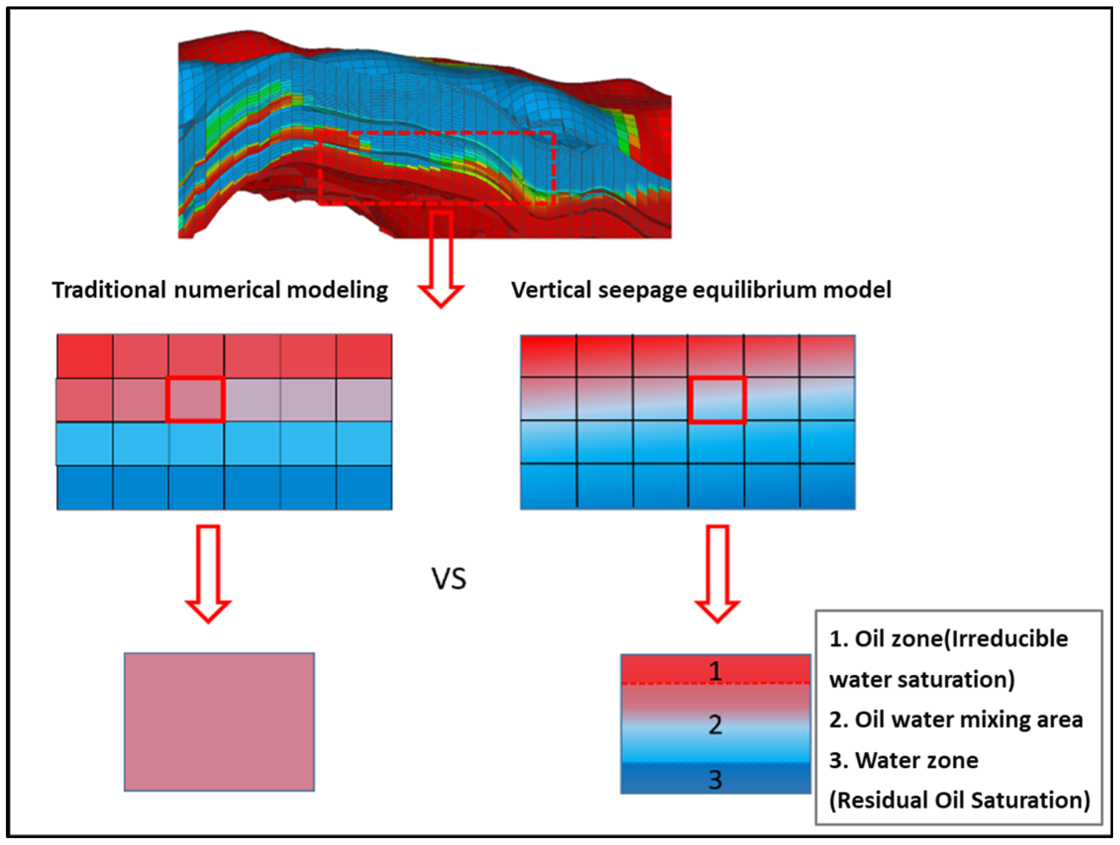
As shown in Figure 1, the diagram represents the difference between the vertical permeability equilibrium model and the ordinary model within numerical simulation grids. In numerical simulation models of gas–water or oil–water systems, it is assumed that the water saturation at the gas–water or oil–water interface grid is equal to 50%. If vertical permeability equilibrium occurs within a grid, the gas–water or oil–water mixture within the grid will be divided into two parts: the upper part of the grid will have a gas or oil saturation equal to the maximum gas or oil saturation (1—bound water saturation), while the lower part of the grid will have a water saturation equal to the maximum water saturation (1—residual gas or residual oil saturation). However, the average water saturation within the grid remains at 50%.

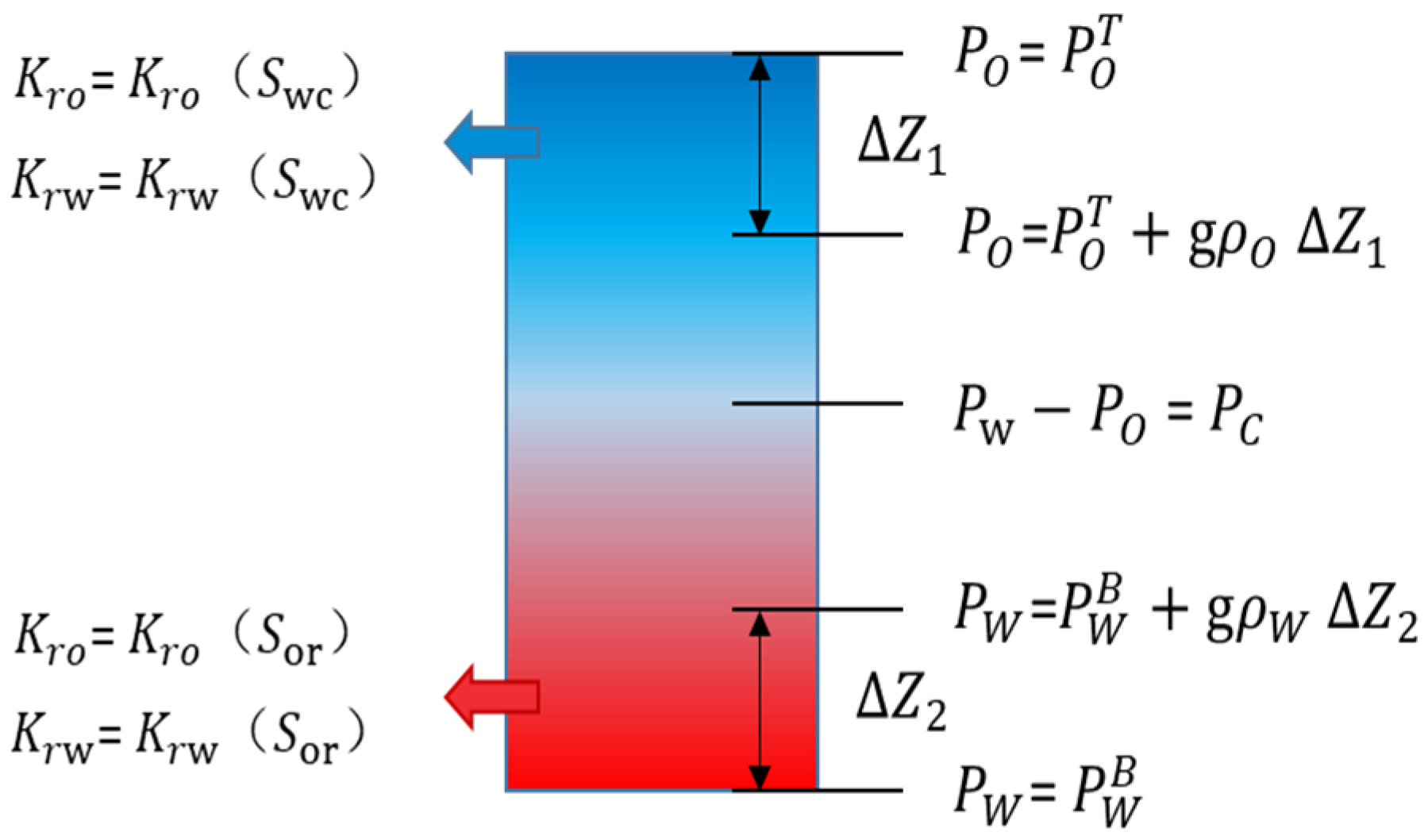
In the numerical model, when a single grid satisfies the vertical flow equilibrium condition and achieves vertical flow equilibrium, the overall saturation of the single grid appears as a fixed value. However, the internal fluid distribution within the grid has changed, leading to alterations in fluid pressure distribution and relative permeability distribution, as illustrated in Figure 2. Upon satisfying the vertical flow equilibrium, the grid undergoes mass exchange with its surroundings under external forces. When fluid moves upwards, the relative permeability of gas, water, or oil–water equals that of the bound water state. Conversely, when fluid moves downwards, the relative permeability of gas, water, or oil–water equals that of the residual gas or residual oil state. Additionally, there are differences in the pressure distribution between the vertical flow equilibrium grid and the conventional grid. Due to varying fluid densities above and below the gas, water, or oil–water interface, gas-phase or oil-phase density is selected for calculating pressure gradients in the upper part of the gas, water, or oil–water interface, while water-phase density is chosen for computing pressure gradients in the lower part of the gas, water, or oil–water interface.

The discriminant conditions for the vertical equilibrium assumption determine the prerequisites for the application of vertical equilibrium numerical models. There are two methods to determine whether the numerical model reaches vertical equilibrium, namely the velocity discriminant condition and the time discriminant condition. Although Becker [22] pointed out that the two commonly used discriminant conditions for vertical equilibrium have obvious shortcomings and local discriminant conditions for near-well and middle reservoir regions have been established, they have not been widely applied. Among them, the velocity discriminant condition can be further categorized into geometric number condition, gravity number condition, and capillary number condition, as follows:

Gravity number condition:

$$N_G=H{k}_h({\rho }_w-{\rho }_o)/L{\mu }_{o}q\approx 1$$

(1)

Capillary number condition:

$$N_{CT}=\sqrt{K_V}/H{N}_{ca}\ge \frac{\delta }{\epsilon },\epsilon =H/L,\sigma =K_v/K_H$$

(2)

Calculation method for the time criterion [39]:

$$t_{seg}=\frac{H\varphi (1-s_{wr}){\mu }_w}{k_{rw}{k}_{v}g({\rho }_w-{\rho }_n)}$$

(3)

where $H$ is the vertical length of the grid; ϕ is reservoir porosity; $s_{wr}$ is wetting phase residual saturation; ${\mu }_w$ is wetting phase viscosity; $k_{rw}$ is wetting phase relative permeability; $k_v$ is vertical absolute permeability; g is gravitational acceleration; ${\rho }_w$ is wetting phase density; and ${\rho }_n$ is non-wetting phase density. If the time step in the numerical simulation is longer than $t_{seg}$, vertical equilibrium occurs.

From a strict standpoint, the time discrimination condition aligns better with physical significance [22,23]. Hence, in this study, we select the C14 block in the Shengli Oilfield as the object to establish the geological model. We calculate the vertical equilibrium time for each grid using the time discrimination condition formula. The C14 block was developed in 1964 and has been in operation for 60 years. In 1993, it entered a high-water cut development period, and by 2011, it had reached the late stage of high-water cut development. In 2018, some blocks had a comprehensive water cut of 98.5%, leading to the shutdown of 173 wells due to high water content, and some reservoir units were close to abandonment. In July 2007, during on-site well inspection, it was discovered that the casing valve of well C14-51 was leaking, resulting in crude oil leakage. Inspired by this incident, oil was directly released from the annular space and transported using tankers, a method later referred to as casing replacement oil production technology. C14-51 started using casing replacement oil production in 2007, and to date, it has produced approximately 10,000 tons of oil with a comprehensive water cut of only 31.3%. Compared to traditional pump extraction, although casing replacement oil production has produced only one-tenth of the oil volume in half the time, it has transformed from being ineffective to effective and highly profitable. C14-51 is a typical example of casing replacement oil production, but not an exception. In this oilfield, casing replacement oil production technology has been used to reuse 20 shut-in wells, resulting in a cumulative oil production of 40,000 tons over 10 years with a comprehensive water cut of 30%.

2.1. Experimental Testing for Determining the Vertical Seepage Equilibrium Time of Porous Sandstone Reservoirs

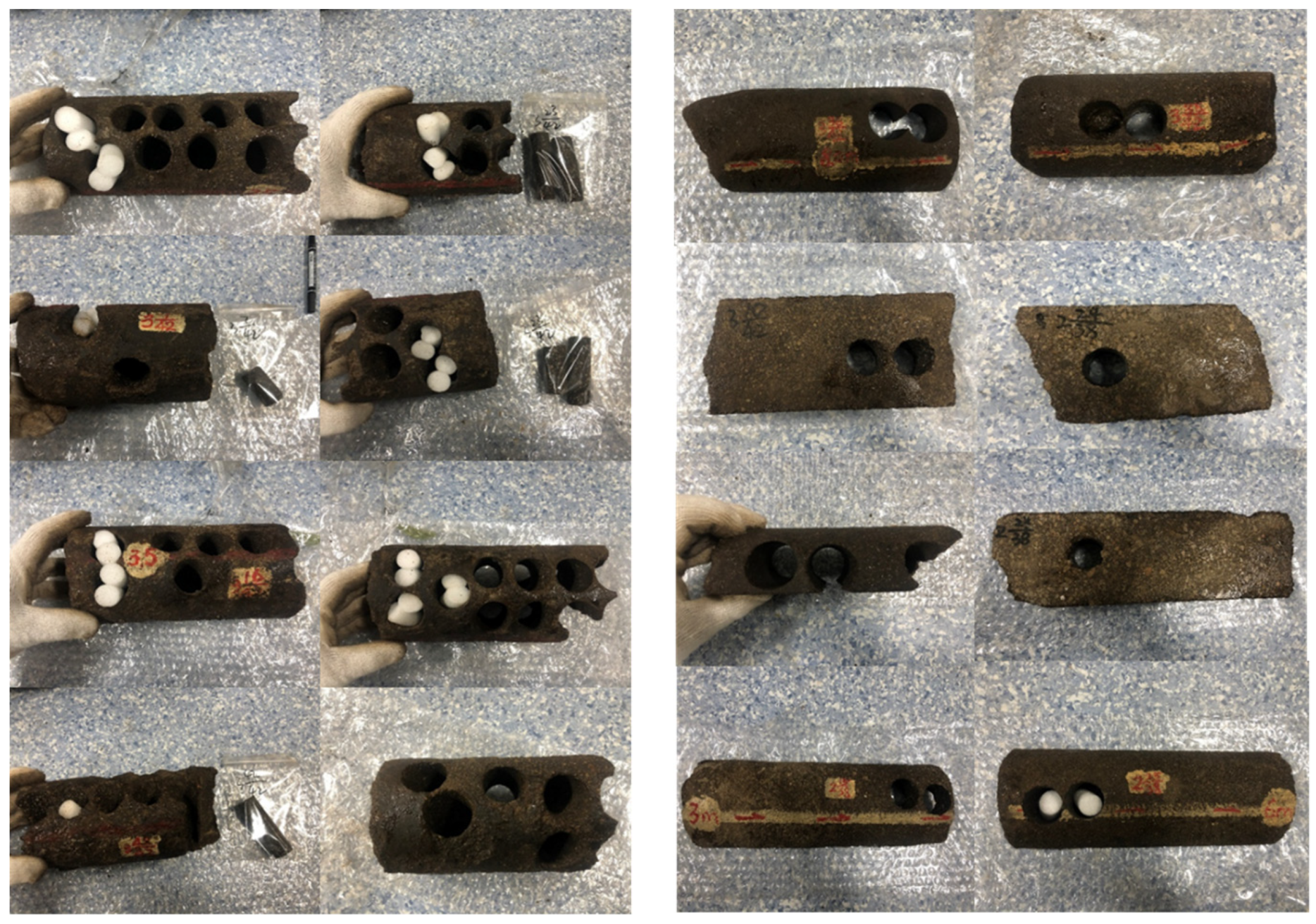
The porous sandstone reservoirs in Shengli Oilfield exhibit significant vertical heterogeneity. Due to the notable differences in permeability along the vertical direction, the vertical migration behavior of oil and water differs greatly from that of conventional reservoirs. The process and conditions required to achieve vertical equilibrium are inevitably different from those of conventional reservoirs. Therefore, relying solely on traditional, time-discriminant methods to determine whether porous sandstone reservoirs meet vertical equilibrium standards is challenging. Addressing the lack of basis for calculating the vertical seepage equilibrium time in porous sandstone reservoirs, this paper conducts vertical seepage equilibrium experiments on five representative core samples selected from real cores at different depths in Shengli Oilfield (see Figure 3). The specific parameters of the five cores are shown in

Table 1. Core parameter value table.

Number	Drilling Core Depth	Logging Depth	Permeability (mD)
1	1189.47	1189.65	2523.24
2	1210.64	1210.82	2291.40
3	1235.26	1235.44	2009.56
4	1256.16	1256.34	1857.72
5	1277.25	1277.43	1695.88

.

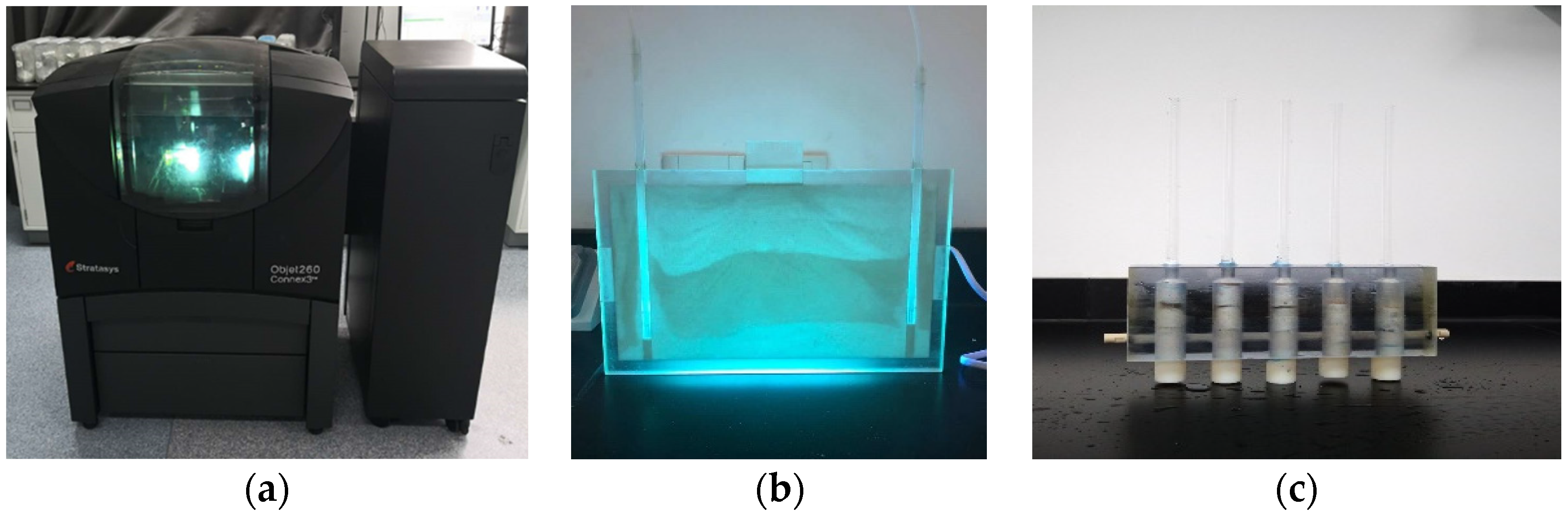
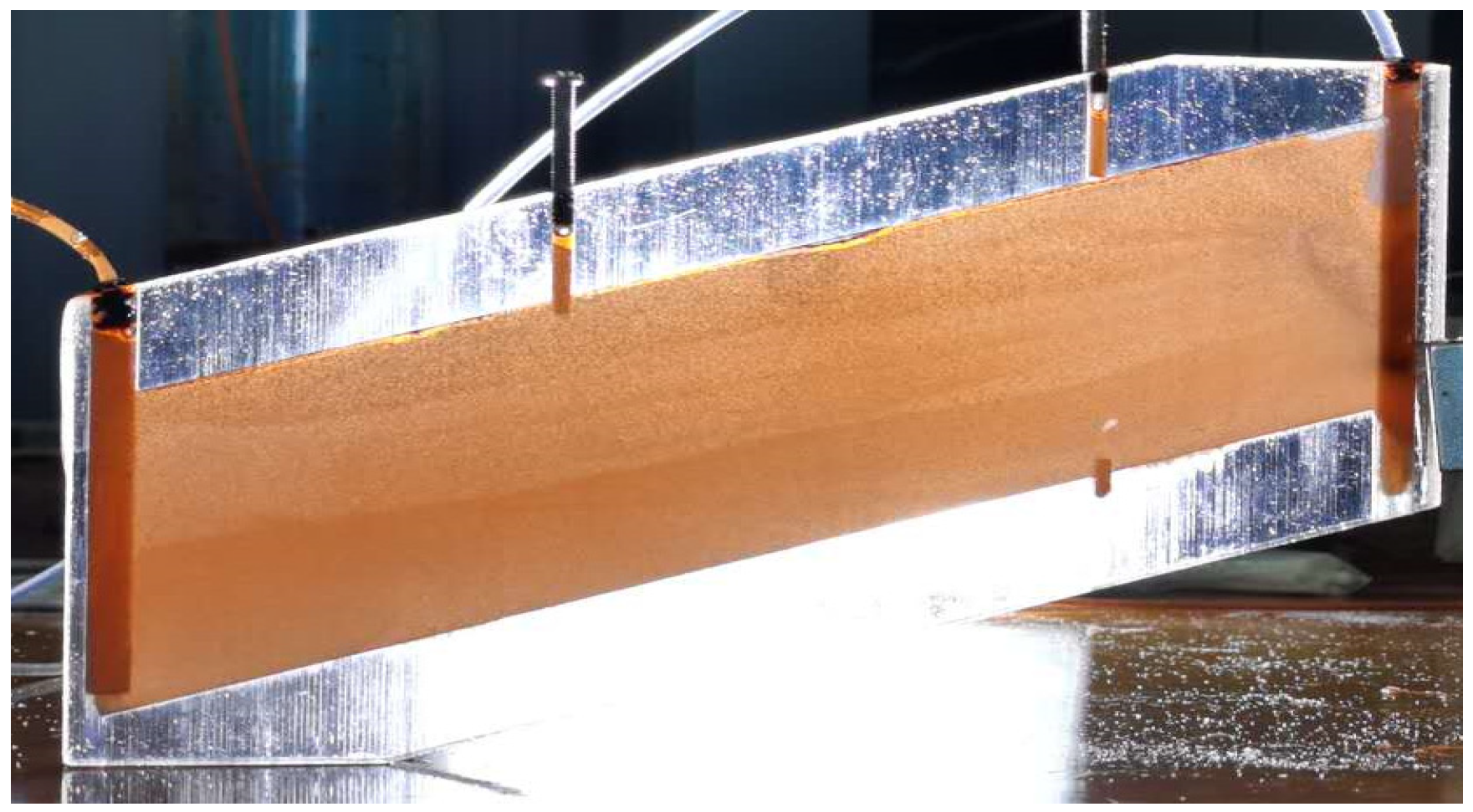
In order to more accurately observe the oil-water migration process, this paper used the EDEN260 CONNEX3 3D printer produced by STRATASYS, Rehovot, Israel, to create a 3D visual unconsolidated sandstone gripper. The model resolution of this 3D printer is 16 microns. The OBJET EDEN260 employs PolyJet, the most advanced 3D printing technology available. This technology involves layer-by-layer jetting of photosensitive resin material onto the print tray, using ultraviolet light to cure each layer during the jetting process until the component is completely manufactured. The printer supports various printing materials, including rigid, opaque materials, rubber-like materials (elastic), transparent materials, high-temperature-resistant materials, polypropylene-like materials, and biocompatible materials. The materials used in this experiment are VeroClear Fullcure 810 high-transparent photosensitive resin and SUP705B soluble support material produced by the Israeli company STRATASYS. The 3D printer and experimental model are shown in Figure 4.

Experimental procedure and steps:

(1)

Select 5 natural cores with consistent lengths but varying permeabilities from the eight cores available.

(2)

Utilize a 3D printer to print a model capable of holding the five cores with different permeabilities. Ensure that channels are created at the top and sides of the model to allow for fluid inflow and outflow.

(3)

Evacuate the cores to absolute vacuum and saturate them with water until they are completely filled. Then, displace the water with oil of varying viscosities to achieve oil saturation, followed by water flooding until reaching residual oil saturation. Place the cores into the holder.

(4)

Inject oil through the channels at the side of the model, targeting the bottom of the cores. Allow the model to settle and observe the upward movement of oil in the glass tube connected to each core to assess the impact of permeability on oil–water migration and draw conclusions.

2.2. Analysis of Vertical Flow Equilibrium Time Test Results in Loose Sandstone Reservoirs

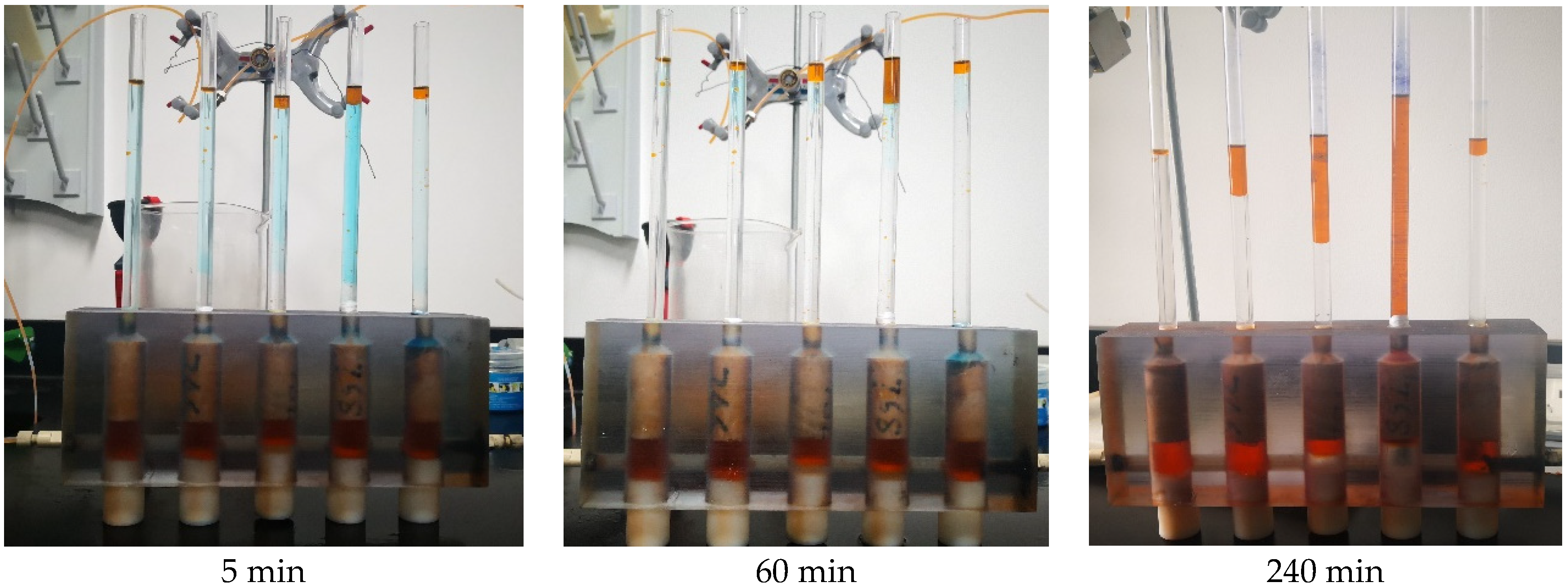
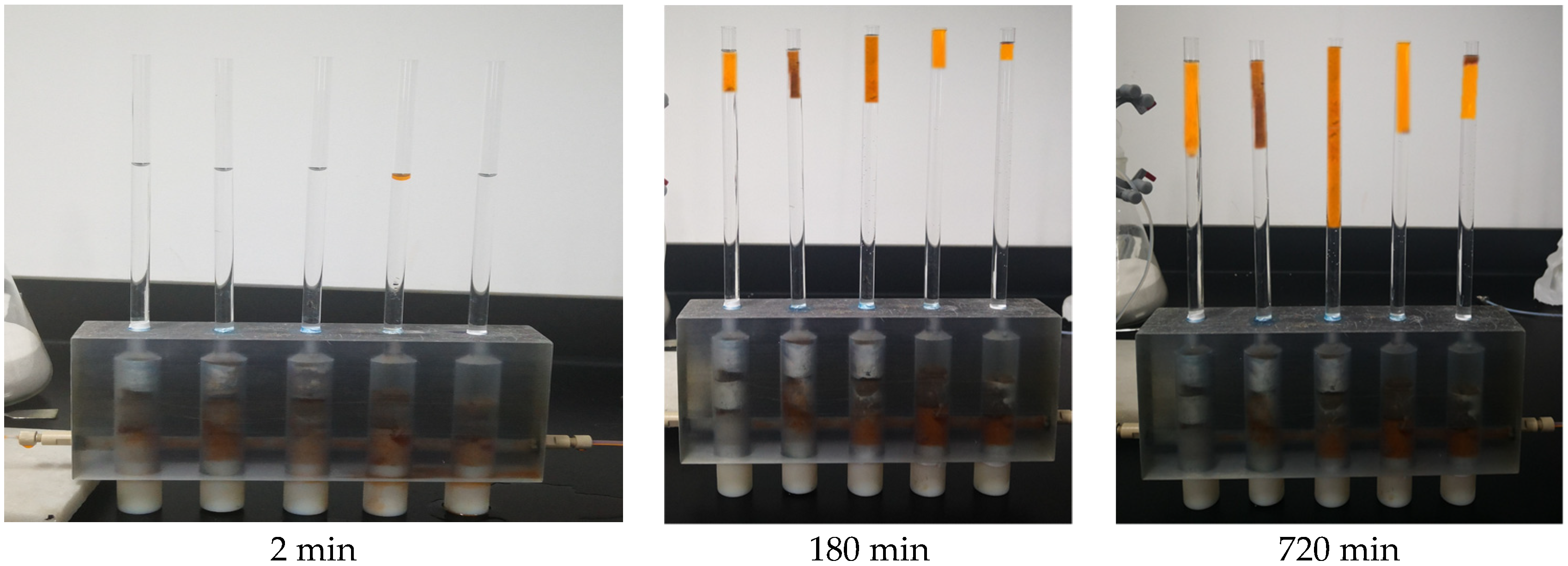
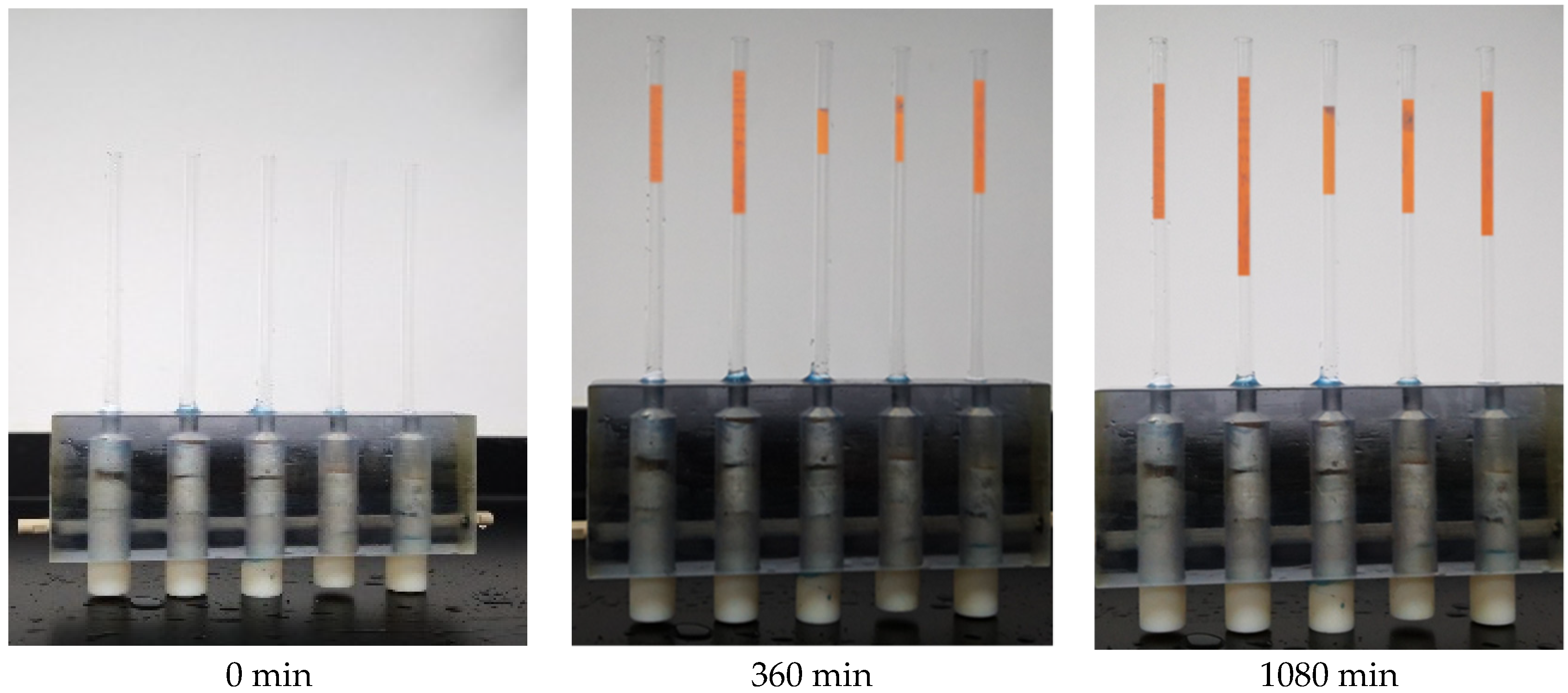
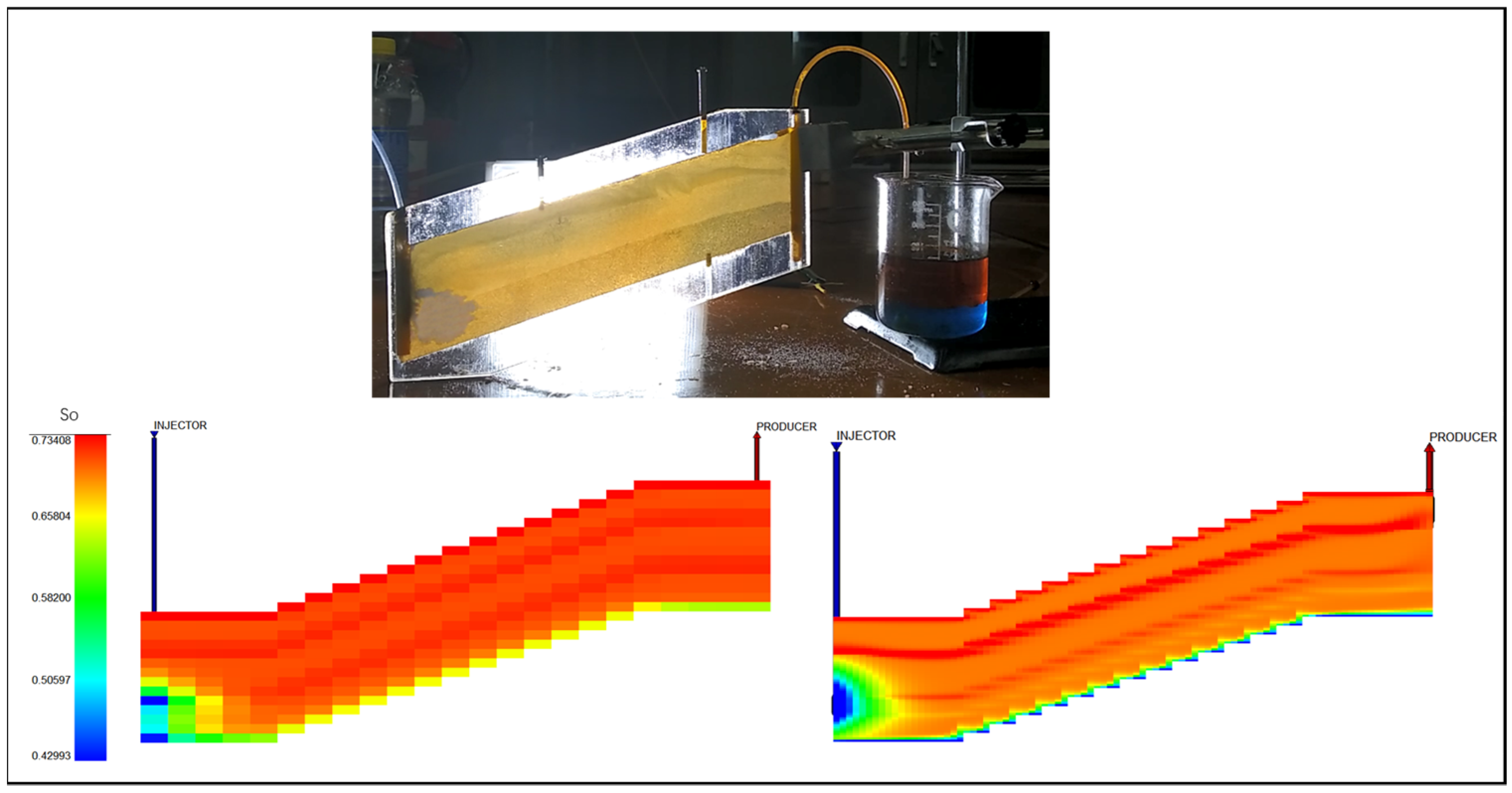
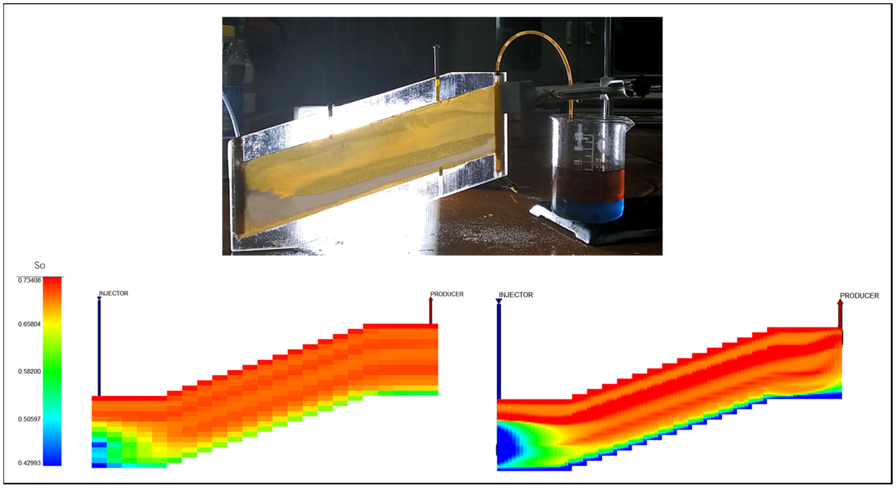
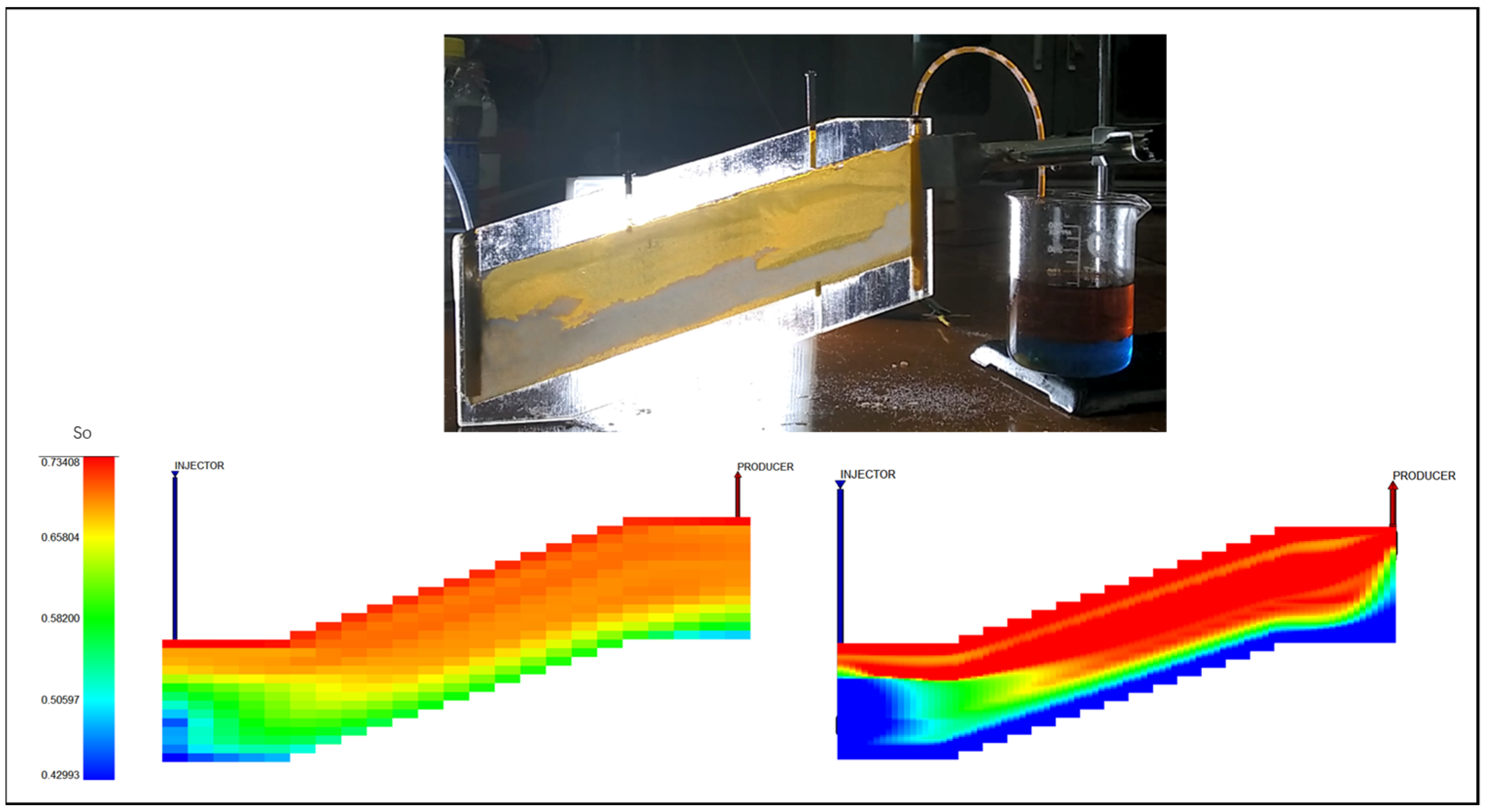
The vertical equilibrium process images of the loose sandstone model with original oil viscosities of 5, 10, and 15 mPa·s and an original oil content of 20 mL during the vertical equilibrium time test experiment for five different permeability loose sandstone cores are shown in Figure 5, Figure 6 and Figure 7, respectively. From the experimental images, it can be observed that the vertical equilibrium process in the loose sandstone reservoir occurs rapidly, and the equilibrium time of oil–water two-phase fluids increases with decreasing core permeability.

Through vertical equilibrium experiments with cores of different permeabilities, the equilibrium time of oil and water in the vertical direction under different viscosities and concentrations of crude oil can be obtained. The specific experimental results are shown in

Table 2. Vertical seepage equilibrium test results.

Number	Permeability (mD)	Viscosity of Crude Oil (mPa·s)	Crude Oil Content (mL)	Vertical Seepage Equilibrium Time (h)
1	2523.24	5	10	3.45
2	2523.24	10	10	7.24
3	2523.24	15	10	10.5
4	2523.24	5	20	4.63
5	2523.24	10	20	12.32
6	2523.24	15	20	18.88
7	2291.40	5	10	3.85
8	2291.40	10	10	7.75
9	2291.40	15	10	11.2
10	2291.40	5	20	5.82
11	2291.40	10	20	13.83
12	2291.40	15	20	20.81
13	2009.56	5	10	4.46
14	2009.56	10	10	8.56
15	2009.56	15	10	12.12
16	2009.56	5	20	7.48
17	2009.56	10	20	15.89
18	2009.56	15	20	23.06
19	1857.72	5	10	4.81
20	1857.72	10	10	9.14
21	1857.72	15	10	12.93
22	1857.72	5	20	8.47
23	1857.72	10	20	17.36
24	1857.72	15	20	25.02
25	1695.88	5	10	5.27
26	1695.88	10	10	9.77
27	1695.88	15	10	13.82
28	1695.88	5	20	9.83
29	1695.88	10	20	19.04
30	1695.88	15	20	27.25

. It can be observed from the experiments that as the viscosity of the crude oil increases, the interfacial tension between oil and water increases, making vertical movement more difficult and resulting in a longer time for complete vertical equilibrium to occur. Additionally, as the concentration of crude oil increases, the distance required for the vertical equilibrium movement of oil and water increases, resulting in a longer time for complete vertical equilibrium to occur. Furthermore, the lower the permeability of the core, the more difficult the vertical movement of oil and water is, leading to a longer time for complete vertical equilibrium to occur.

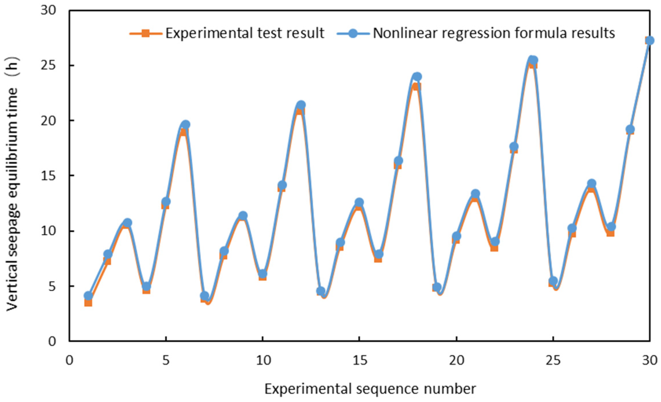
Based on the results of 30 sets of experiments on vertical seepage equilibrium time, a formula for calculating the vertical seepage equilibrium time was obtained using a multivariate nonlinear regression method, as shown in Equation (4).

y = −0.66 − 0.006x₁ + 0.864x₂ + 1.298x₃ − 0.00027x₁x₂ − 0.0004975x₁x₃ + 0.08x₂x₃ + 0.00000255x₁² − 0.016x₂² − 0.012x₃²

(4)

In the above equation, y represents the vertical equilibrium time in hours; x₁ denotes the reservoir permeability in millidarcies (mD); x₂ stands for the viscosity of crude oil in millipascal-seconds (mPa·s); and x₃ represents the volume of crude oil in milliliters (mL). By plotting the results of the 30 sets of vertical seepage equilibrium time experiments against the calculated results from Equation (4) in Figure 8 it can be observed that Equation (4) exhibits a high degree of fitting accuracy, with a correlation coefficient reaching 0.999.

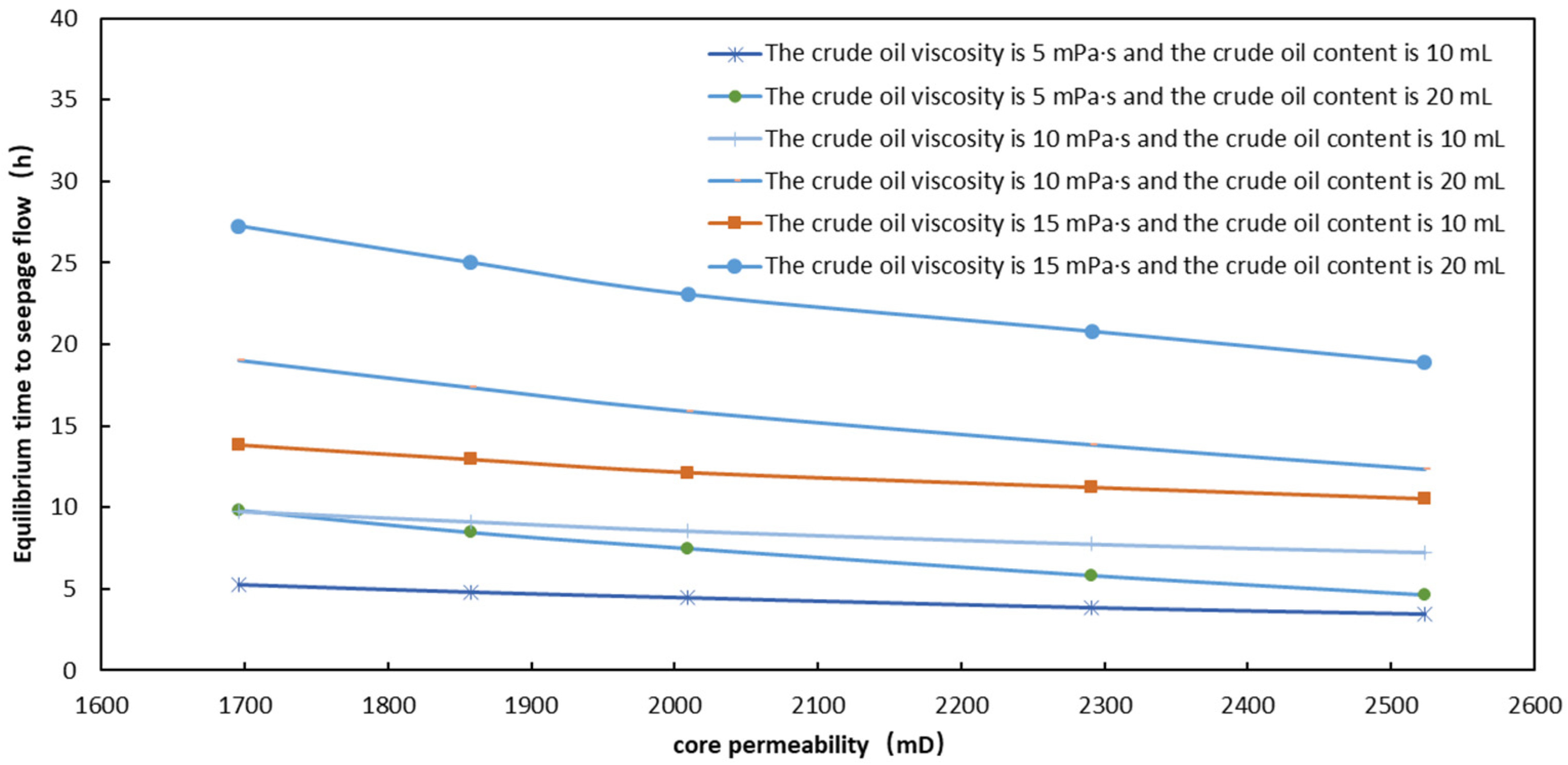
Using the multivariate nonlinear regression method, the formula for calculating the vertical seepage equilibrium time in loose sandstone reservoirs was derived. Through this formula, the vertical seepage equilibrium time for different viscosities and volumes of crude oil in various permeability cores can be obtained, as shown in Figure 9. In the simulation model of the Victory Oilfield, the vertical grid height ranges from 2 m to 5 m, and the viscosity of the crude oil is 5 cp. The calculation reveals that the time for vertical equilibrium is approximately 15 days, which is significantly shorter than the time step of 30 days used in numerical simulations. Additionally, it is also shorter than the calculation results obtained using existing theoretical formulas.

3. Numerical Simulation Method for Loose Sandstone Reservoirs Considering Vertical Seepage Equilibrium Mechanism

The basic equations of the numerical simulation model for loose sandstone reservoirs considering the mechanism of vertical seepage equilibrium are divided into three parts: governing equations, transport equations, and auxiliary equations. Building upon the gas–water two-phase grid reconstruction method developed by Guo et al. [22], this study established a numerical simulation method suitable for oil–water two-phase flow in loose sandstone reservoirs.

3.1. Non-Miscible Vertical Seepage Equilibrium Numerical Simulation Method

If the dissolution process of one fluid in another is ignored, the governing equation for immiscible fluids in porous media is as follows:

$$\frac{\partial {\rho }_w\varphi s_w}{\partial t}+\nabla \cdot ({\rho }_w{\overrightarrow{u}}_w)={\rho }_w{q}_w$$

(5)

$$\frac{\partial {\rho }_o\varphi s_o}{\partial t}+\nabla \cdot ({\rho }_o{\overrightarrow{u}}_o)={\rho }_o{q}_o$$

(6)

Considering rigid solids and incompressible fluids, the governing equation can be simplified into the following:

$$\frac{\partial \varphi s_w}{\partial t}+\nabla \cdot {\overrightarrow{u}}_w=q_w$$

(7)

$$\frac{\partial \varphi s_o}{\partial t}+\nabla \cdot {\overrightarrow{u}}_o=q_o$$

(8)

The equation of motion of the oil phase and the water phase is as follows:

$${\overrightarrow{u}}_o=-\frac{k{k}_{ro}}{{\mu }_o}\nabla (p_o-{\rho }_{o}g\Delta z)$$

(9)

$${\overrightarrow{u}}_w=-\frac{k{k}_{rw}}{{\mu }_w}\nabla (p_w-{\rho }_{w}g\Delta z)$$

(10)

The auxiliary equation is as follows:

$$s_w+s_o=1$$

(11)

$$p_o=p_w+p_c(s_w)$$

(12)

If vertical seepage equilibrium occurs, then the two-phase fluid of gas and water or oil and water will achieve complete gravitational separation in the vertical direction, with capillary force and gravity in equilibrium. Once vertical equilibrium occurs in a numerical simulation grid, the saturation distribution and pressure distribution within the grid no longer need to be numerically solved; they can be calculated based on the conservation of mass equation.

By integrating the governing equation along the vertical direction as follows:

$${\int }_{z_B}^{z_T}[\frac{\partial s_{\alpha {\rho }_{\alpha }\varphi }}{\partial t}+\nabla \cdot (\alpha {\overrightarrow{u}}_{\alpha })]dz={\int }_{z_B}^{z_T}{\rho }_{\alpha }{q}_{\alpha }dz$$

(13)

where α = w,o is the phase, and the subscripts T and B represent the top and bottom, respectively.

Assuming that both fluid and rock are incompressible, ignoring the vertical change in fluid density, the above formula is expanded and simplified to obtain the following:

$$\begin{array}{c}{\int }_{z_B}^{z_T}\frac{\partial s_{\alpha {\rho }_{\alpha }\varphi }}{\partial t}dz={\rho }_{\alpha }\frac{\partial }{\partial t}{\int }_{z_B}^{z_T}{s}_{\alpha }\varphi dz+{\int }_{z_B}^{z_T}\varphi s_{\alpha }\frac{\partial {\rho }_{\alpha }}{\partial t}dz{\int }_{z_B}^{z_T}\frac{\partial s_{\alpha {\rho }_{\alpha }\varphi }}{\partial t}dz\\ {=\rho }_{\alpha }\frac{\partial }{\partial t}{\int }_{z_B}^{z_T}{s}_{\alpha }\varphi dz+\frac{\partial {\rho }_{\alpha }}{\partial t}{\int }_{z_B}^{z_T}\varphi s_{\alpha }dz{\int }_{z_B}^{z_T}\frac{\partial s_{\alpha {\rho }_{\alpha }\varphi }}{\partial t}dz\\ ={\rho }_{\alpha }\frac{\partial }{\partial t}{\int }_{z_B}^{z_T}{s}_{\alpha }\varphi dz+{\rho }_{\alpha }{c}_{\alpha }{\int }_{z_B}^{z_T}\varphi s_{\alpha }dz\end{array}$$

(14)

$$\begin{array}{c}{\int }_{z_B}^{z_T}\nabla \cdot \left(\alpha {\overrightarrow{u}}_{\alpha }\right)dz={\int }_{z_B}^{z_T}\left(\nabla {\rho }_{\alpha }{\overrightarrow{u}}_{\alpha }+{\rho }_{\alpha }\nabla {\overrightarrow{u}}_{\alpha }\right)dz={\rho }_{\alpha }{\int }_{z_B}^{z_T}\left({\nabla }_{\parallel }{\overrightarrow{u}}_{\alpha ,\parallel }+{\nabla }_{\perp }{\overrightarrow{u}}_{\alpha ,\perp }\right)dz\\ ={\rho }_{\alpha }({\nabla }_{\parallel }{\int }_{z_B}^{z_T}{\overrightarrow{u}}_{\alpha ,\parallel }dz+u_{\alpha ,\perp }-u_{\alpha ,B})\end{array}$$

(15)

$$\frac{\partial }{\partial t}{\int }_{z_B}^{z_T}{s}_{\alpha }\varphi dz+c_{\alpha }{\int }_{z_B}^{z_T}\varphi s_{\alpha }dz+{\nabla }_{\parallel }{\int }_{z_B}^{z_T}{\overrightarrow{u}}_{\alpha ,\parallel }dz+u_{\alpha ,\perp }-u_{\alpha ,B}={\int }_{z_B}^{z_T}{q}_{\alpha }dz$$

(16)

where $c_{\alpha }=\frac{1}{{\rho }_{\alpha }}\frac{d{\rho }_{\alpha }}{d{P}_{\alpha }}$ is the fluid compression coefficient and $u_{\alpha ,T}$ and $u_{\alpha ,B}$ are the top and bottom flow rates of the α phase, respectively. $\parallel$ is the (x,y) plane and is perpendicular; $P_{\alpha }$ is the pressure of α phase in the coarse grid, and the pressure at $z_B$ at the bottom of the grid is taken here.

According to the vertical equilibrium hypothesis, the fluid phase pressure has a hydrodynamic static equilibrium relationship, as shown in the following equation:

$$p_{\alpha }(x,y,z,t)=P_{\alpha }(x,y,t)+{\rho }_{\alpha }g(z-z_B)$$

(17)

The sagging integral variables are expressed as follows:

$$\Phi (x,y)={\int }_{z_B}^{z_T}\varphi (x,y,z)dz$$

(18)

$$S_{\alpha }(x,y,t)=\frac{1}{\Phi }{\int }_{z_B}^{z_T}\varphi (x,y,z)s_{\alpha }(x,y,z,t)dz$$

(19)

$${\overrightarrow{U}}_{\alpha }={\int }_{z_B}^{z_T}{\overrightarrow{u}}_{\alpha ,\parallel }dz$$

(20)

$$Q_{\alpha }={\int }_{z_B}^{z_T}{q}_{\alpha }dz$$

(21)

$$K={\int }_{z_B}^{z_T}{k}_{\parallel }dz$$

(22)

$${\mathsf{\Lambda }}_{\alpha }=K^{-1}{\int }_{z_B}^{z_T}{k}_{\parallel }{\lambda }_{\alpha }dz$$

(23)

where ${\lambda }_{\alpha }=\frac{k_{r\alpha }}{{\mu }_{\alpha }}$ is the fluidity of α phase.

After substituting the above integral variables into the governing equation and the equation of motion and sorting them out, we can obtain the following:

$$\frac{\partial (\Phi S_{\alpha })}{\partial t}+c_{\alpha }\Phi S_{\alpha }\frac{\partial P_{\alpha }}{\partial t}+{\nabla }_{\parallel }\cdot {\overrightarrow{U}}_{\alpha }=Q_{\alpha }-(u_{\alpha ,T}-u_{\alpha ,B})={\Psi }_{\alpha }$$

(24)

$${\overrightarrow{U}}_{\alpha }=-K{\mathsf{\Lambda }}_{\alpha }({\nabla }_{\parallel }{P}_{\alpha }-{\rho }_{\alpha }g\Delta z)$$

(25)

By solving the above vertical integral two-dimensional equations, the saturation Sα and phase pressure P_α of the coarse mesh can be obtained, and the corresponding phase saturation and phase pressure distributions of the fine mesh can be reconstructed by vertical equilibrium calculation.

The vertical equilibrium model assumes that the fluid instantaneously reaches gravitational equilibrium, so its application depends on the relationship between the actual vertical equilibrium time $t_{seg}$ and the numerical simulation time step T. If $t_{seg}$ is much smaller than T, then the vertical equilibrium model usually provides a good approximation; otherwise, the vertical equilibrium model is not applicable. The vertical equilibrium model has the advantage of high computational efficiency. To extend its applicability, this paper proposes an anisotropic multiscale vertical equilibrium calculation model, which still adopts the vertical integration concept but considers the dynamic changes of the anisotropy of the two-phase fluid in both the plane and vertical directions. This is referred to as the dynamic anisotropic vertical equilibrium method. In this section, we first introduce the grid reconstruction method, then derive the control equations for the anisotropic coarse scale and fine scale, and finally provide the numerical solution process.

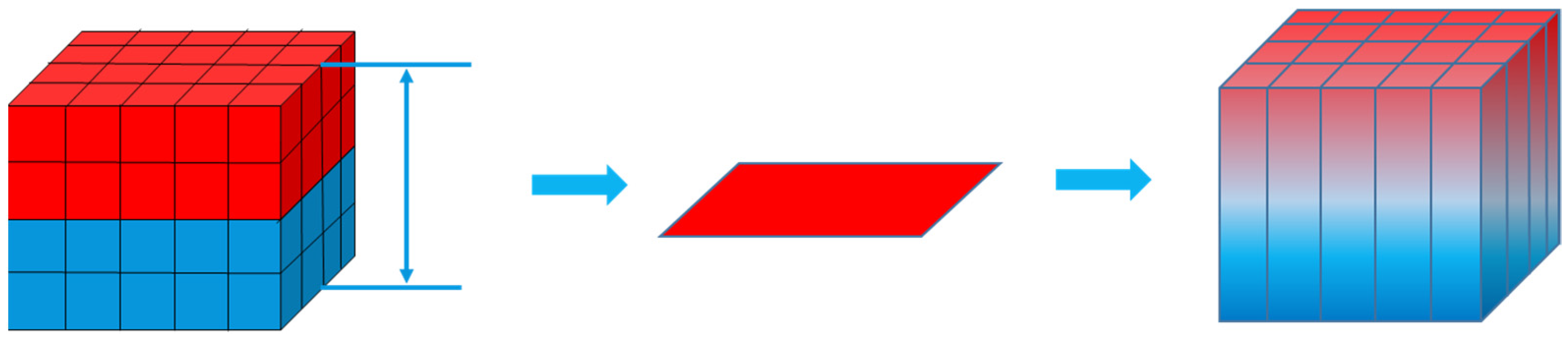
The grid reconstruction method involves two scales: the plane two-dimensional domain after coarse-scale vertical integration and the one-dimensional domain within the fine-scale vertical range, as shown in Figure 10.

Under the coarse-scale model, the coarse-scale phase pressure is $P_{\alpha }(x,y,t)$. Can be obtained by solving the vertical integral equation. On this basis, the fine-scale phase saturation can be obtained by solving the phase saturation equation (shunt equation).

The governing equations of the whole grid reconstruction method are divided into two parts: the vertical integral two-dimensional equation for coarse-scale phase pressure and a series of one-dimensional equations for fine-scale state quantities. The following coarse-scale equation is the result of the addition of two-phase vertical integral equations:

$$(c_{\varphi }H+c_w\Phi )S_w\frac{\partial P_w}{\partial t}+(c_{\varphi }H+c_o\Phi )S_o\frac{\partial P_o}{\partial t}+{\nabla }_{\parallel }\cdot ({\overrightarrow{U}}_w+{\overrightarrow{U}}_o)={\Psi }_w+{\Psi }_o$$

(26)

where $H$ is the thickness of coarse-scale mesh and $c_{\varphi }=\frac{d\varphi }{dp}$ is the pore compression factor of the rock.

It is important to note that the mobility in the grid reconstruction model is defined the same as in the traditional vertical equilibrium model. However, unlike the traditional vertical equilibrium model, in the grid reconstruction model, mobility requires numerical integration to account for the fine-scale mobility. Additionally, the coarse-scale capillary force in the grid reconstruction model differs from the pseudo-capillary force used in the traditional vertical equilibrium model. In the traditional vertical equilibrium model, strict hydrodynamic static equilibrium assumptions are imposed on the two-phase fluids to reconstruct the vertical pressure profile. Due to the restrictive nature of these assumptions, a more general pressure reconstruction method is proposed in this paper. Based on the vertical equilibrium concept, the pressure reconstruction function is defined as follows:

$$p_{\alpha }(x,y,z,t)=P_{\alpha }(x,y,t)+{\pi }_{\alpha }(x,y,z,t)$$

(27)

Using this reconstructed pressure, the integral flow rate $U_{\alpha }$ can be calculated by computing the gradient of the function $p_{\alpha }$ in the horizontal direction, thereby solving the integral control equation to obtain the coarse-scale phase pressure $P_{\alpha }$. The specific calculation process will be discussed in the next section. Here, we focus on introducing the reconstruction function ${\pi }_{\alpha }$.

Taking into account practical applications, the reconstruction function should meet the following requirements: ease of computation, physical significance, and the ability to revert to the vertical equilibrium model under certain conditions. After multiple experiments, the current preferred method is the saturation-weighted pressure function for two phases, as shown below:

$$\frac{\partial p_o}{\partial z}=-(s_w{\rho }_w+s_o{\rho }_o)g+s_w\frac{\partial p_c(s_w)}{\partial z}$$

(28)

$$\frac{\partial p_w}{\partial z}=-(s_w{\rho }_w+s_o{\rho }_o)g-s_o\frac{\partial p_c(s_w)}{\partial z}$$

(29)

Taking the water phase as an example, the pressure reconstruction equation is as follows:

$$p_w(x,y,z,t)=P_w(x,y,t)-{\int }_{z_B}^z[(s_w{\rho }_w+s_o{\rho }_o)g+s_o\frac{\partial p_c(s_w)}{\partial z}]dz$$

(30)

In the fine-scale model, the material conservation equation is reconstituted as follows:

$$\frac{\partial ({\rho }_{\alpha }\varphi s_{\alpha })}{\partial t}+\frac{\partial ({\rho }_{\alpha }{u}_{\alpha ,z})}{\partial z}={\rho }_{\alpha }{q}_{\alpha }-{\nabla }_{\parallel }\cdot ({\rho }_{\alpha }{\overrightarrow{u}}_{\alpha ,\parallel })$$

(31)

In the equation, $u_{\alpha ,z}$ represents the vertical velocity of phase $\alpha$, and ${\overrightarrow{u}}_{\alpha ,\parallel }$ represents the horizontal velocity of phase$\alpha$. Under different flow velocities, the shape of the relative permeability curve for oil–water two-phase flow varies. However, using a single set of permeability curves to represent the migration behavior of oil and water in traditional vertical equilibrium models is inaccurate. Building upon the relevant research findings from the team led by Wang Shuoliang, this study incorporates dynamic relative permeability curves to characterize the migration behavior of oil and water in reservoirs with different permeabilities.

After solving the coarse scale model and reconstructing the fine scale pressure profile, ${\overrightarrow{u}}_{\alpha ,\parallel }$ can be obtained by the following formula:

$${\overrightarrow{u}}_{\alpha ,\parallel }=-k_{\parallel dynamic}{\lambda }_{\alpha dynamic}{\nabla }_{\parallel }{p}_{\alpha }$$

(32)

The relative permeability of oil and water is affected by velocity. In this paper, $k_{\parallel dynamic}$ of the above formula is written as a function of velocity and saturation when dealing with dynamic permeability.

The governing equation of the fine-scale model is expanded and organized into the following:

$$\varphi \frac{\partial s_{\alpha }}{\partial t}+(c_{\varphi }+\varphi c_{\alpha })s_{\alpha }\frac{\partial p_{\alpha }}{\partial t}+\frac{\partial u_{\alpha ,z}}{\partial z}=q_{\alpha }-{\nabla }_{\parallel }\cdot {\overrightarrow{u}}_{\alpha ,\parallel }$$

(33)

By adding the governing equations of the two phases and eliminating the saturation, the pressure equation can be obtained as follows:

$$(c_{\varphi }+\varphi c_w)s_w\frac{\partial p_w}{\partial t}+(c_{\varphi }+\varphi c_o)s_o\frac{\partial p_o}{\partial t}+\frac{\partial u_{TOT,z}}{\partial z}=q_w+q_o-{\nabla }_{\parallel }\cdot ({\overrightarrow{u}}_{w,\parallel }+{\overrightarrow{u}}_{o,\parallel })$$

(34)

By solving this equation, the total vertical velocity can be obtained as follows:

$$u_{TOT,z}=u_{w,z}+u_{o,z}$$

(35)

The flow velocity of the oil and water phases can be obtained separately in the form of the diverting quantity of Darcy’s law, as follows:

$$u_{w,z}=f_w\cdot (u_{TOT,z}-k_z{\lambda }_o\Delta \rho g+k_z{\lambda }_o\frac{\partial p_c}{\partial z})$$

(36)

$$u_{o,z}=f_o\cdot (u_{TOT,z}+k_z{\lambda }_w\Delta \rho g-k_z{\lambda }_w\frac{\partial p_c}{\partial z})$$

(37)

where $f_{\alpha }=\frac{{\lambda }_{\alpha }}{{\lambda }_w+{\lambda }_o}$ is the shunt function and $\Delta \rho ={\rho }_o-{\rho }_w$ is the difference between oil and water density.

After obtaining$u_{\alpha ,z}$, ${\overrightarrow{u}}_{\alpha ,\parallel }$, and $p_{\alpha }$, the fine-scale saturation distribution $s_{\alpha }$ can be reconstructed by solving the governing equation of the fine-scale model.

3.2. Calculation Method

The spatial discretization of the dynamic anisotropic vertical equilibrium model was performed using the standard cell-centered finite volume method. For temporal discretization, a method similar to the Implicit Pressure Explicit Saturation (IMPES) method was adopted: pressure was implicitly handled at the coarse scale, while saturation was explicitly handled at the fine scale, decoupling the two scales. Therefore, the coarse-scale pressure was first solved implicitly, followed by an explicit computation of the fine-scale saturation.

The governing equation of the coarse-scale model is numerically discretized as follows:

$$\begin{array}{l}(c_{\varphi }H+c_w\Phi S_w^n+c_o\Phi S_o^n)\frac{P_w^{n+1}-P_w^n}{\Delta t}+(c_{\varphi }H+c_o\Phi )S_o^n\frac{P_c^n-P_c^{n-1}}{\Delta t}\\ -{\nabla }_{\parallel }\cdot \left\{K\right[({\mathsf{\Lambda }}_w^n+{\mathsf{\Lambda }}_o^n)\cdot {\nabla }_{\parallel }{P}_w^{n+1}+{\mathsf{\Lambda }}_o^n{\nabla }_{\parallel }{P}_c^n]+{\int }_{z_B}^{z_T}{k}_{\parallel }({\mathsf{\Lambda }}_w^n{\nabla }_{\parallel }{\pi }_w^n+{\mathsf{\Lambda }}_o^n{\nabla }_{\parallel }{\pi }_o^n)dz\}={\Psi }_w^{n+1}+{\Psi }_o^{n+1}\end{array}$$

(38)

where n represents time $t^n$. This system of equations is linear and can be solved directly to obtain $P_w^{n+1}$.

In order to solve the governing equation of the fine-scale model, it is necessary to first calculate the horizontal phase flow rate as follows:

$${\overrightarrow{u}}_{\alpha ,\parallel }^{n+1,\ast }=-k_{\parallel }{\lambda }_{\alpha }^n\cdot {\nabla }_{\parallel }{p}_{\alpha }^{n+1,\ast }$$

(39)

Use $p_{\alpha }^{n+1,\ast }(x,y,z,t)=P_{\alpha }^{n+1}(x,y,t)+{\pi }_{\alpha }^n(x,y,z,t)$ for reconstructing fine scale pressure. Moreover, the superscript * is expressed as an approximation at time $t^{n+1}$.

Discretize the pressure equation on a fine scale as follows:

$$\frac{\partial u_{TOT,z}^{n+1,\ast }}{\partial z}=-{\nabla }_{\parallel }\cdot {\overrightarrow{u}}_{TOT,\parallel }^{n+1,\ast }+q_w^{n+1}+q_o^{n+1}-(c_{\varphi }+\varphi c_w)s_w^n\frac{p_w^{n+1,\ast }-p_w^n}{\Delta t}-(c_{\varphi }+\varphi c_o)s_o^n\frac{p_c^{n+1,\ast }-p_c^n}{\Delta t}$$

(40)

Use $u_{TOT,\parallel }^{n+1,\ast }=u_{w,\parallel }^{n+1,\ast }+u_{o,\parallel }^{n+1,\ast }$ by the fine-scale model of the vertical velocity of $u_{TOT,z}^{n+1,\ast }$, and then calculate the oil–water two-phase shunt volume:

$$u_{w,z}^{n+1,\ast }=f_w^n\cdot (u_{TOT,z}^{n+1,\ast }-k_z{\lambda }_o^n\Delta \rho g+k_z{\lambda }_o^n\frac{\partial p_c^n}{\partial z})$$

(41)

$$u_{o,z}^{n+1,\ast }=f_o^n\cdot (u_{TOT,z}^{n+1,\ast }+k_z{\lambda }_w^n\Delta \rho g-k_z{\lambda }_w^n\frac{\partial p_c^n}{\partial z})$$

(42)

Plug it into the governing equation of the fine-scale model as follows:

$$\varphi \frac{s_{\alpha }^{n+1}-s_{\alpha }^n}{\Delta t}+(c_{\varphi }+\varphi c_{\alpha })s_{\alpha }^n\frac{p_{\alpha }^{n+1,\ast }-p_{\alpha }^n}{\Delta t}+\frac{\partial u_{\alpha ,z}^{n+1,\ast }}{\partial z}=q_{\alpha }^{n+1}-{\nabla }_{\parallel }\cdot {\overrightarrow{u}}_{\alpha ,\parallel }^{n+1,\ast }$$

(43)

The fine-scale phase saturation distribution $s_{\alpha }^{n+1}$ can be calculated.

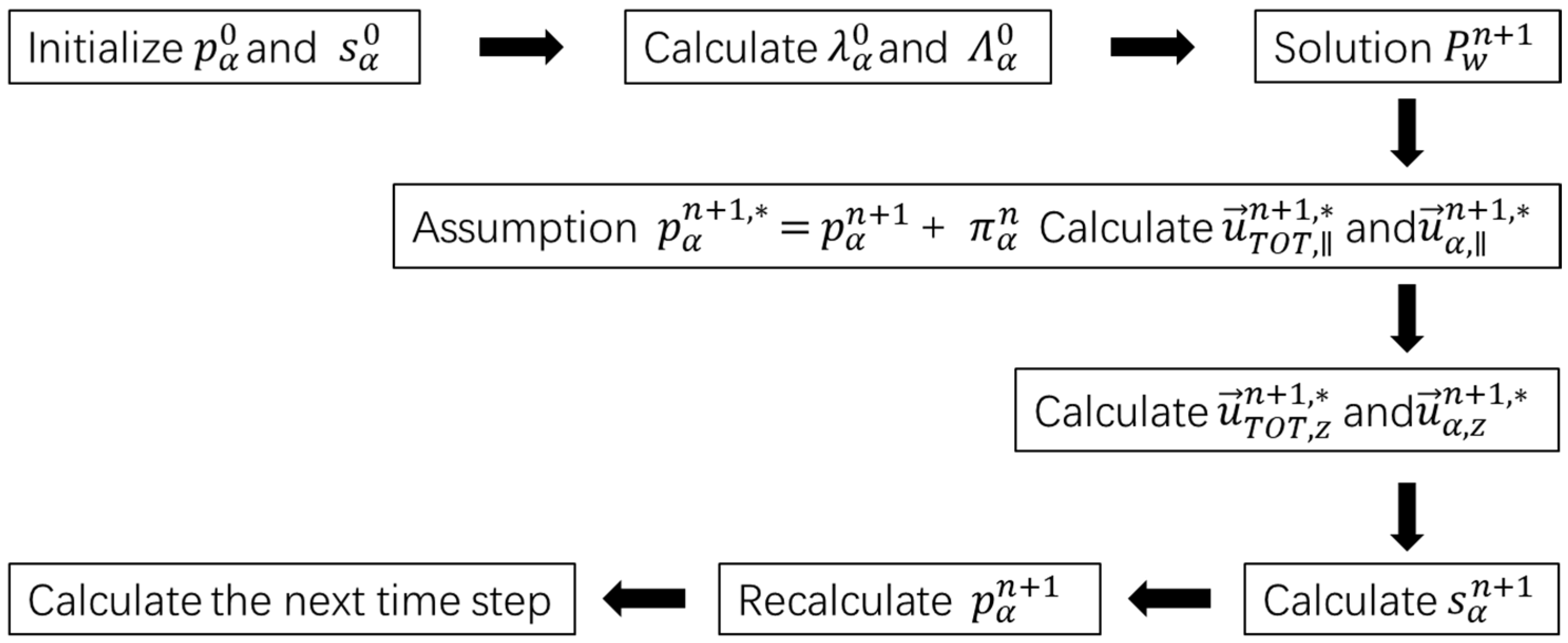
Finally, an updated vertical pressure distribution can be obtained as follows:

$$p_w^{n+1}=P_w^{n+1}-{\int }_{z_B}^z[(s_w^{n+1}{\rho }_w+s_o^{n+1}{\rho }_o)g+s_o^{n+1}\frac{\partial p_c(s_w^{n+1})}{\partial z}]dz$$

(44)

$$p_o^{n+1}=P_w^{n+1}+P_c^{n+1}-{\int }_{z_B}^z[(s_w^{n+1}{\rho }_w+s_o^{n+1}{\rho }_o)g-s_w^{n+1}\frac{\partial p_c(s_w^{n+1})}{\partial z}]dz$$

(45)

The entire calculation process is as follows (Figure 11):

4. The Impact of Vertical Seepage Equilibrium Time on Numerical Simulation Methods: Experimental Comparison and Accuracy Analysis

The Mutual Verification of Numerical Simulation Results and Physical Simulation Results

To validate the applicability and accuracy of the numerical simulation method proposed in this paper, considering the dynamic anisotropic vertical equilibrium mechanism, physical simulation experiments of one injection and one production displacement in loose sandstone were conducted. A three-dimensional numerical simulation model with dimensions consistent with the experimental results and a physical simulation model were established for comparison. By comparing the results of the physical simulation experiments with the numerical simulation calculations, the differences between traditional numerical simulation methods and numerical simulation methods considering vertical equilibrium were analyzed to verify the accuracy of the latter.

In the physical simulation experiments, a 3D-printed visualized sand-filled model was utilized. The model’s bottom end served as the injection end, while the middle of the other end served as the production end, conducting one-injection and one-production displacement experiments. The experimental model is shown in Figure 12. The displacement employed the same oil as mentioned earlier, with a viscosity of 5 mPa·s, and deionized water was used for injection (Figure 12).

The specific experimental steps were as follows:

• Open the injection end and production end of the model. Utilize a constant-speed cross-flow pump to inject oil into the model’s injection end at a rate of 1 mL/min until the model is fully saturated with oil.
• Replace the fluid at the injection end with water and inject water into the model at a rate of 1 mL/min. Record the amount of produced water and oil at the production end.
• Continuously take photographs using a camera and record the entire process with a video recorder to document the water-oil displacement at different time points.

In this study, two numerical simulation methods were employed: the traditional oil–water two-phase numerical simulation method and the numerical simulation method considering vertical equilibrium. The specific parameters of the numerical simulation model are shown in

Table 3. Physical simulation model basic parameter value table.

Parameter	Value of Number	Parameter	Value of Number
Number of model grids	10 × 3 × 10	Horizontal X-direction grid step size (cm)	2.6
Vertical step length (cm)	1.1	Model initial oil saturation	1
Model initial pressure (MPa)	0.1	Model injection–production well	Bottom injection, top mining
Model porosity	0.3	Model permeability (μm2)	1000, 1500, and 2000

.

Comparisons between the results of the two numerical simulation methods and the observed photos from the physical experiments are presented together in Figure 13, Figure 14 and Figure 15.

By comparing the numerical simulation results with the physical experiment results at the same time points, it can be observed that the numerical simulation model considering the anisotropic vertical flow equilibrium is more consistent with the actual physical experiment results. After water injection into the reservoir, rapid gravitational segregation of oil and water occurs at the front of the water drive, with water flowing along the bottom of the model while the top layer of oil remains largely unaffected. In contrast, the traditional numerical simulation model of oil–water two-phase flow exhibits significant discrepancies in the longitudinal distribution of oil and water due to the lack of consideration for the anisotropic vertical equilibrium of the reservoir. Particularly around the injection and production wells, the differences in oil–water distribution are most pronounced, with the traditional numerical model failing to reflect the movement pattern of the oil–water interface. A comparison of the mid-section grids reveals that in the model, considering the anisotropic vertical equilibrium of the reservoir, injected water primarily migrates through the lower part of the reservoir. In contrast, in the traditional numerical simulator, the range of water penetration in the vertical direction is significantly greater than that in the model considering vertical equilibrium, resulting in the displacement and penetration of oil in the vertical direction, which is inconsistent with the actual physical simulation results. Therefore, considering the numerical simulation method for vertical equilibrium can more accurately describe the movement laws of oil and water phases in porous sandstone reservoirs.

5. Conclusions

(1)

This study utilized 3D printing technology to fabricate a visualized core holder and sand-filled model, obtaining the vertical equilibrium time of oil and water phases in porous sandstone models. Through multivariate nonlinear regression, a calculation method for the vertical equilibrium time of porous sandstone reservoirs was established.

(2)

Starting from the vertical seepage equilibrium mechanism of fluids, a mathematical model for the two-phase flow of oil and water in porous sandstone reservoirs was established. Additionally, a multi-scale vertical seepage equilibrium grid reconstruction method was introduced, enabling the decoupled calculation of fluid saturation and pressure profiles on coarse and fine-scale grids.

(3)

A three-dimensional numerical model consistent with the visualized physical model of porous sandstone reservoirs was established. The oil–water profiles calculated using this method were compared with the results of a single injection and a single production experiment. The results indicate that the vertical seepage equilibrium model can more accurately describe the distribution patterns and migration states of oil–water two-phase fluids in the longitudinal direction of the reservoir, validating the reliability of the method.