Numerical Investigation on the Aerodynamic and Aeroacoustic Characteristics in New Energy Vehicle Cooling Fan with Shroud

Abstract

The cooling fan is one of the important noise sources for new energy vehicles, and the research on its aerodynamic and aeroacoustic characteristics is of great help to improve the noise, vibration and harshness performance of new energy vehicles. However, most of these studies focus on the impeller, and little consideration has been given to the study of the shroud. Based on the coupling calculation method of large eddy simulation and the Ffowcs-Williams and Hawkings acoustics model, the aerodynamic and aeroacoustic characteristics in a cooling fan with the shroud are investigated at flow rates from 0.623 kg/s to 1.019 kg/s (where 0.865 kg/s is the flow rate corresponding to the best efficiency point). The accuracy of numerical simulation results is verified by the grid independence verification and the comparison of experimental data. Research shows that several large-scale vortex structures are observed in the clearance between the impeller and the shroud. The maximum peak-to-peak values of pressure fluctuation at different flow rates occur in the intermediate section or outlet section of the shroud. Although the shroud contributes relatively less to the far field noise, its different distribution may change the position of the maximum sound pressure level. The dominant frequency of pressure fluctuation equals the blade passage frequency (BPF) and the maximum SPL is around the BPF, both of which are independent of flow rates. The maximum SPL and the amplitude of the dominant frequency decrease as the flow rate increases.

1. Introduction

New energy vehicles are an important means of transport for environmental protection and energy conservation and can be an effective alternative to conventional vehicles. New energy vehicles, especially pure electric vehicles, omit the exhaust device and a large number of transmission components are driven by electric motors. As a result, the requirements for the performance of noise, vibration and harshness (NVH) are significantly improved, which has become a hot research direction for new energy vehicles. The present study focuses on the research of noise sources and noise mechanisms.

The cooling fan is one of the main noise sources of new energy vehicles [1,2]. The aeroacoustic characteristics of cooling fans are determined by their aerodynamics, such as flow separation, secondary flow and other special flow structures. A large number of studies have been performed on aerodynamic characteristics [3,4,5,6,7,8,9] and aeroacoustic characteristics [10,11,12,13,14,15,16]. For example, Nashimoto et al. [3] used phase-averaged PIV measurement and found that the separation and reattachment of the flow occurred on the suction surface at the leading edge of the blade. Marcus et al. [4] found that the clearance flow flows out of the clearance and then towards the blade, resulting in strong pressure fluctuations at the tip of the blade. Bo et al. [5] found that there is leakage flow in the tip clearance and high-velocity region on the suction side near the blade tip. Zhao et al. [6] compared the vortex strength of the blade tips with different tip clearances and found that the proximity of a shroud mitigates tip vortices. Mo et al. [10] found that there is a strong tonal noise at the leading edge of the blades with a high sound pressure level (SPL). Wang et al. [11] found that the vortex at the trailing edge of the blades has high turbulent kinetic energy and the vortex noise generated is also of great concern. Park et al. [12] used a hybrid approach with a URANS CFD and acoustic analogy and found a significant low-frequency broadband noise at the leading edge of the blade tip. In addition, components adjacent to the blades can also be affected to produce higher noise. Lim et al. [13] found that the clearance between the blades and the casing created tip vortices, which generate high SPLs at the surfaces of the struts of the casing.

Since the cooling fan is one type of axial fan, several investigations also have been concentrated on high-speed axial fans [17], low-speed axial fans [18,19,20], low-pressure axial fans [21,22], and hollow blade axial fans [23,24]. Hu et al. [25] conducted an FW-H acoustic simulation on high-speed axial flow fans, and the results showed that the noise on the blade pressure surface was greater than that on the suction surface. Moosania et al. [18] analyzed the flow structure of a low-speed partially shrouded fan and found that there are low-speed zones at the hub and blade tip. This phenomenon causes higher noise to be generated in the outer part of the blades [21]. However, Eberlinc et al. [23] reduced the adverse flow phenomenon at the trailing edge of the blade tip by using hollow blades.

Although the aerodynamic and aeroacoustic characteristics of cooling fans (even axial fans) have been studied, most of them are concentrated on the fan impeller. Few studies have considered the impact of shroud [25,26], whose mechanism has not been clearly revealed. A detailed understanding requires data regarding the cooling fan with the shroud. With the development of computational fluid dynamics, large-eddy simulation (LES) is used in the community because it is a powerful tool to obtain abundant flow field and pressure fluctuation [10,22]. Combined with the FW-H model method, detailed and accurate noise data can be obtained also.

Therefore, the present study takes a cooling fan with a shroud used in new energy vehicles as the research object. Then, numerical simulations of the research object under flow rates of 0.623 kg/s to 1.019 kg/s (where 0.865 kg/s is the flow rate corresponding to the best efficiency point) are performed. The influence of flow rate on the aerodynamic and aeroacoustic characteristics is investigated in detail.

2. Geometric Model and Numerical Descriptions

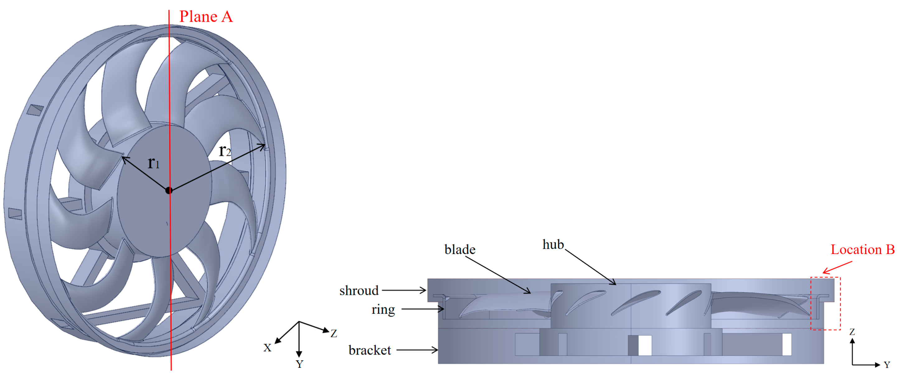
2.1. Geometric Model of Cooling Fan

This model is a simplified cooling fan for new energy vehicles, consisting of blades, hub, ring, bracket and shroud, as shown in Figure 1.

Table 1. Main parameter of the cooling fan.

Specification	Value
r1 (mm)	80
r2 (mm)	180
Rotation speed of impeller (rpm)	2770
Number of blades, Z	9

lists the specifications of the cooling fan. The fan has a total of nine forward swept blades with radii of 80 mm and 180 mm from center to hub and blade tip, respectively. The fan has a total of nine forward swept blades with radii of 80 mm and 180 mm from center to hub and blade tip, respectively. The fan speed is 2770 rev/min.

A part (location B) of the meridian section (plane A) on the fan is designated to observe the flow quantities in the subsequent analysis.

For the convenience of subsequent analysis of pressure fluctuation and noise, Figure 2 shows the locations of monitoring points and acoustic receivers. There are 12 monitoring points (P1~P12) on the shroud wall at location B, which can be divided equally into three parts according to the positions of shroud corners Cl and C2, with the monitoring points evenly spaced in each part. In addition, acoustic receivers are arranged in the far field of the fan. The direction of R3 is the fan inlet, and R9 is the fan outlet. The acoustic receivers are located at 30° intervals, each 1 m from the center of the fan, for a total of 12 acoustic receivers to measure the SPL in the far field of the fan.

For the numerical calculation of the cooling fan, the inlet and outlet domains have been added to the cooling fan, see Figure 3. The inlet field is a hemisphere with a radius of 1200 mm and the outlet field is a rectangle of 2500 mm × 1600 mm × 1500 mm (length × width × height).

2.2. Computational Fluid Dynamics (CFD) Method

With the development of computational fluid dynamics, numerical simulations are widely used in the study of cooling fans. At present, the governing equations are the Navier–Stokes equations for a compressible fluid. The governing equations of continuity and momentum equations in the conservation form are generally written as follows [11]:

$$\frac{\partial \rho }{\partial t}+\frac{\partial }{\partial x_i}\left(\rho u_i\right)=0$$

(1)

$$\frac{\partial \left(\rho u_i\right)}{\partial t}+\frac{\partial \left(\rho u_i{u}_j\right)}{\partial x_j}=F_i-\frac{\partial p}{\partial x_i}+\frac{\partial {\tau }_{ij}}{\partial x_j}$$

(2)

where $\rho$ is the density, $p$ is the pressure, $u_i$ is the velocity vector, $F_i$ is the volume force acting on the fluid and ${\tau }_{ij}$ is the stress tensor.

The steady turbulence is first simulated using the $k-\epsilon$ model [27,28]. Subsequently, using the steady results as the initial flow field, a Large Eddy Simulation based on Smagorinsky–Lilly Model is used to obtain the unsteady turbulence of the cooling fan. This setup has been tested in several studies on rotating machinery [10,29,30].

(1)

$k-\epsilon$ model

The $k-\epsilon$ model is a semi-empirical model, which is a numerical model based on the turbulent kinetic energy k of the model transport equation and its dissipation rate ε [31]. The transport equations for $k$ and $\epsilon$ in the $k-\epsilon$ model are introduced as follows:

$$\begin{array}{c}\frac{\partial }{\partial t}\left(\rho k\right)+\frac{\partial }{\partial x_i}\left(\rho k{u}_i\right)=\frac{\partial }{\partial x_j}\end{array}\left[\left(\mu +\frac{{\mu }_t}{{\sigma }_k}\right)\frac{\partial k}{\partial x_i}\right]+G_k-\rho \epsilon$$

(3)

$$\begin{array}{c}\frac{\partial }{\partial t}\left(\rho \epsilon \right)+\frac{\partial }{\partial x_i}\left(\rho \epsilon u_i\right)=\frac{\partial }{\partial x_i}\end{array}\left[\left(\mu +\frac{{\mu }_t}{{\sigma }_{\epsilon }}\right)\frac{\partial k}{\partial x_i}\right]+C_1\rho S_1-C_2\rho \frac{{\epsilon }^2}{\sqrt{k+\epsilon }}$$

(4)

where, $C_1$ and $C_2$ are constant parameters, ${\sigma }_k$ and ${\sigma }_{\epsilon }$ are the turbulent Prandtl numbers for $k$ and $\epsilon$, $G_k$ refers to the turbulent kinetic energy due to the mean velocity gradient, which is defined by Equation (4) according to the exact transport equation:

$$G_k=-\rho {\overline{u_i}}^{\prime }{\overline{u_j}}^{\prime }\frac{\partial u_j}{\partial x_i}$$

(5)

(2)

Smagorinsky–Lilly Model

Large eddy simulation generates a subgrid stress model for calculation when dealing with small-scale vortices. Using the Smagorinsky–Lilly subgrid stress model, the interaction between the subgrid scale and the grid scale can be likened to the molecular viscosity of Brownian motion so that the eddy-viscosity is modeled by

$${\mu }_t=\rho {L_S}^2\left|\overline{S}\right|$$

(6)

where $\left|\overline{S}\right|=\sqrt{2\overline{S_{ij}} \overline{S_{ij}}}$, $S_{ij}$ is the rate of strain tensor for the resolved scale. $L_S$ is the mixing length for subgrid scales and is defined as follows

$$L_S=\min \left(\kappa d,C_S{V}^{1/3}\right)$$

(7)

where $\kappa$, $d$, $C_S$ is the von Kármán constant, the distance to the closest wall and the Smagorinsky constant, respectively, and $V$ is the volume of the computational cell. For most numerical calculations of fluid flow, $C_S=1$ is ideal in order to reduce the diffusion effects of subgrid stresses [32].

2.3. Ffowcs-Williams and Hawkings (FW-H) Equation

The aerodynamic noise generated from the unsteady flow is predicted by a hybrid approach. In this approach, the LES is coupled with the FW-H acoustics model. The FW-H formulation adopts the most general form of the Lighthill acoustic analogy, which describes the sound generation mechanism of an object moving through a fluid and is able to make predictions about the sound generation of an equivalent acoustic source [33]. The FW-H equation is written in the following form:

$$\begin{array}{r}\frac{1}{a_0^2}\cdot \frac{{\partial }^2{\rho }^{\prime }}{\partial t^2}-{\nabla }^2{p}^{\prime }=\frac{\partial }{\partial t}\left\{\left[{\rho }_0{v}_n+\rho \left(u_n-v_n\right)\right]\delta \left(f\right)\right\}\\ \begin{array}{c}-\frac{\partial }{\partial x_i}\left\{\left[P_{ij}{n}_j+\rho u_i\left(u_n-v_n\right)\right]\delta \left(f\right)\right\}+\frac{{\partial }^2}{\partial x_{i}x}\left(T_{ij}H\left(f\right)\right)\end{array}\end{array}$$

(8)

The first term on the right-hand side of Equation (8) represents the monopole source, determined by the amount of variation in blade surface thickness, the second term represents a dipole source, generated by surface stresses between the fluid and the wall, and the third term represents a quadrupole source, generated by internal stresses in the flow, where quadrupole noise is usually neglected at Mach numbers less than 0.3.

Where $u_n$ is the fluid velocity component perpendicular to the source plane S = 0, $v_n$ is the source plane velocity component in the vertical source plane direction, $a_0^2$ is the far-field sound velocity, $p^{\prime }$ is the sound pressure at the observation point, $\delta \left(f\right)$ is the Dirac function, $H\left(f\right)$ is the Heaviside function and $P_{ij}$ is compressive stress tensor. The Lighthill stress tensor $T_{ij}$ is defined as:

$$\begin{array}{c}{T}_{ij}=\rho u_i{u}_j+P_{ij}-a_0^2\left(\rho -{\rho }_0\right){\delta }_{ij}\end{array}$$

(9)

where ${\delta }_{ij}$ is the Kronecker delta function.

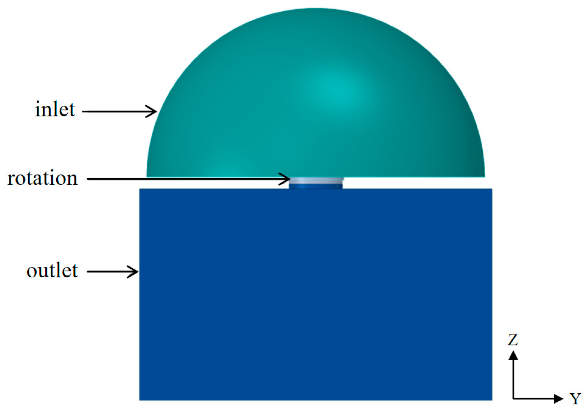
2.4. Numerical Settings

All calculations in this study are carried out using ANSYS FLUENT 18.0. The finite volume method is used for the solution and a pressure-based solver is chosen for the solver type. A second-order upwind format is used to spatially discretize all derivative terms, and the SIMPLE algorithm is used to realize the coupling of pressure and velocity. A high-resolution solution with second-order accuracy is used to ensure the accuracy of the calculation. The overall calculation process is shown in Figure 4.

Air with constant density at 15 °C is chosen as the medium of flow. A rotational coordinate system is set up for the impeller region and a stationary coordinate system for the other components. All wall surfaces in the flow domain are set to be No-slip walls. Mass flow boundary conditions are set at the inlet of the computational domain and pressure-outlet boundary conditions are selected at the outlet.

For the LES calculation, the inlet turbulent intensity is 5%, and the inlet turbulence viscosity rate is 10%. In addition, the time step, $\Delta t=6.017\times {10}^{-5} \mathrm{s}$, which corresponds to one degree of rotation of the fan impeller. The flow fields developed for 1800 time-steps, equivalent to five revolutions of the impeller.

The FW-H model is used for noise analysis of a cooling fan. The surfaces of the impeller and shroud are set as the sound source surfaces. The noise is sampled at a period of 0.11 s, corresponding to five rotations of the fan. The sampling time interval is set to one time-step and a total of 1800 time-steps are calculated, which leads to a frequency resolution of around 9 Hz.

3. Computational Meshes and Experimental Validation

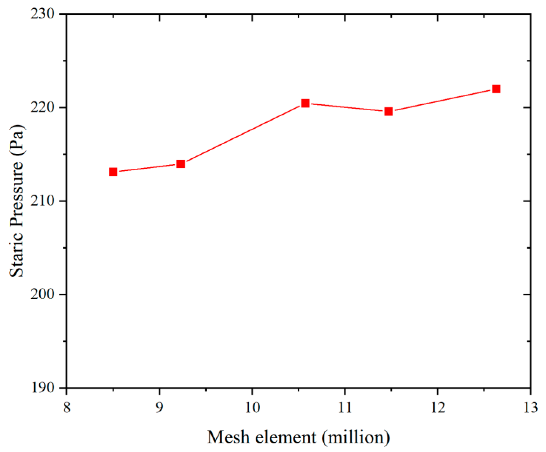
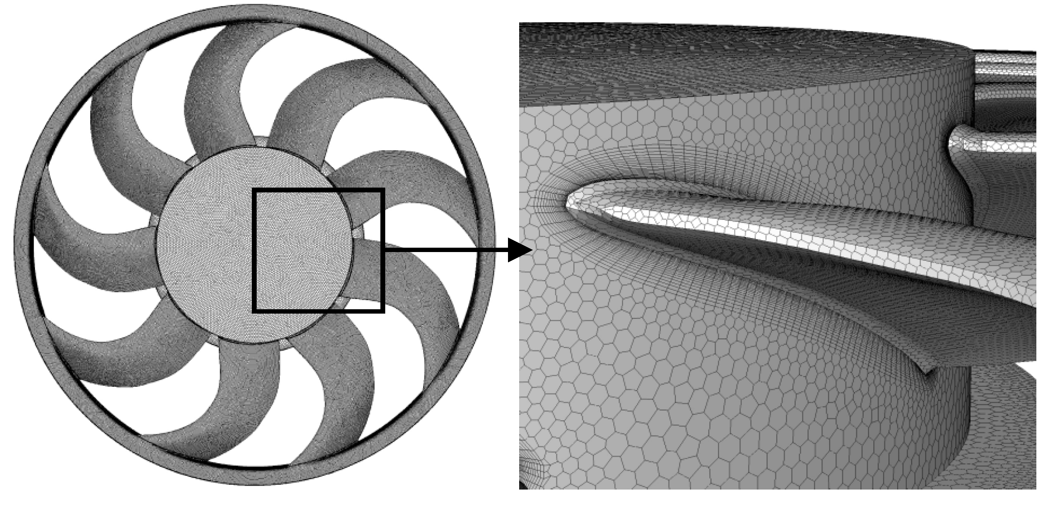
3.1. Evaluation of Mesh Quality

Fluent Meshing 18.0 is used to divide the computational domain into polyhedral meshes, and the near-wall regions are encrypted. Polyhedral meshes have excellent geometric adaptability to produce good-quality meshes on complex geometric models.

The static pressure rise from the inflow and the outflow sections of the fan are selected as the indicator for the grid independence study under a flow rate of 0.729 kg/s. The five mesh numbers, respectively, are approximately 8.5 million, 9.23 million, 10.57 million, 11.47 million and 12.63 million. Moreover, except for the mesh with a minimum size of 1 mm for 8.5 million, the minimum size of all other mesh is 0.5 mm. Figure 5 shows the evolution of static pressure rises with mesh number. As the mesh number increases from 8.5 million to 10.57 million, the static pressure rises to 7.34 Pa; 12.63 million is only 1.53 Pa higher than that at 10.57 million.

Therefore, the mesh number equal to 10.57 million is chosen, of which the rotating domain is approximately 7.2 million and the stationary domain is approximately 3.37 million, as given in

Table 2. Number of grids of the computational domain.

Domain	Number of Grids (104)
Rotating	720
Stationary	337
Total	1057

. The meshes around the cooling fan are shown in Figure 6.

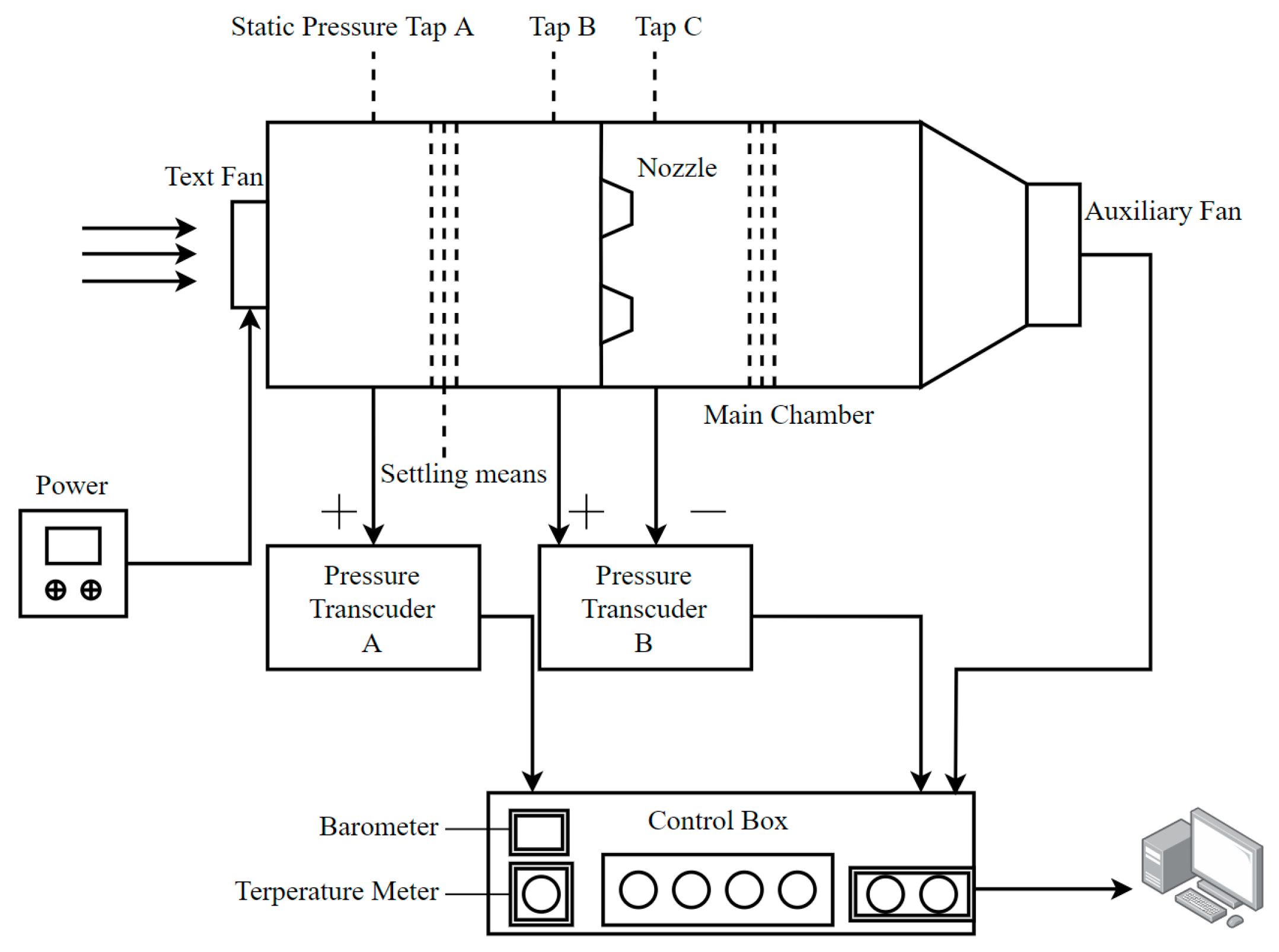
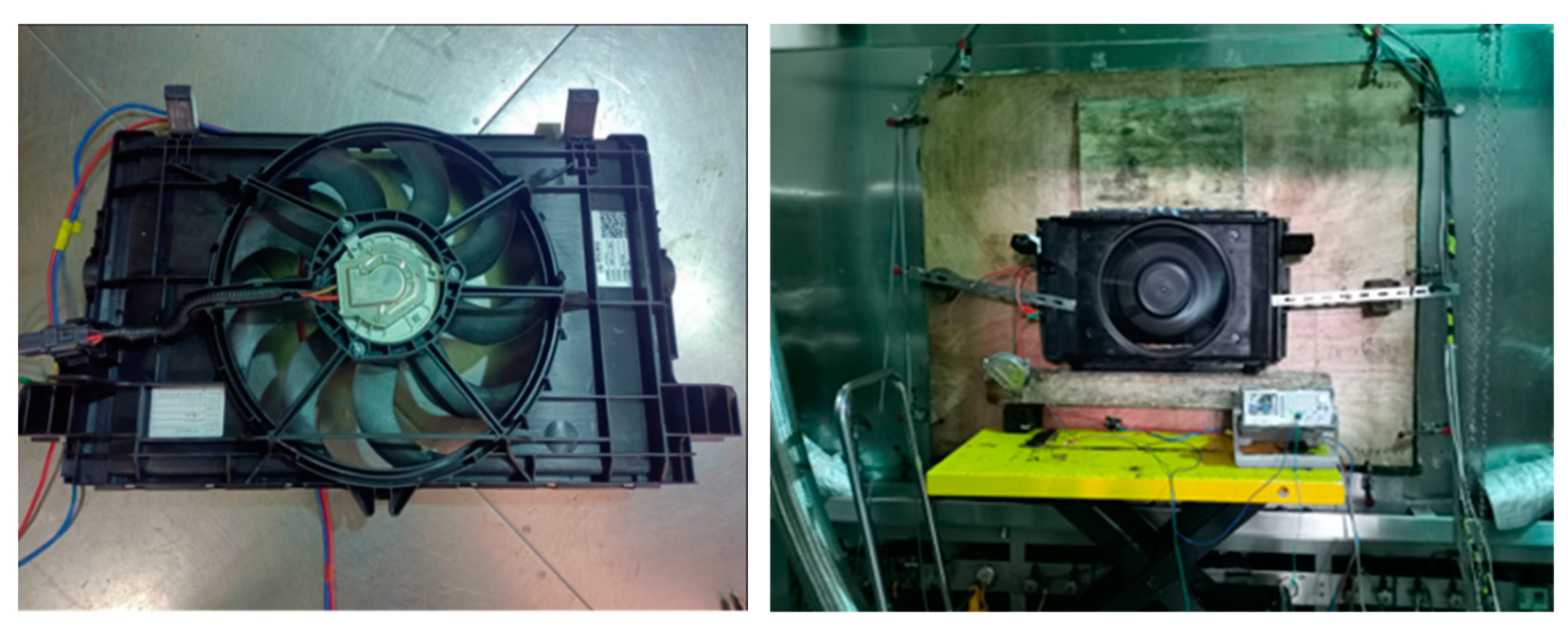
3.2. Experimental Validation

The experimental measurement of the external characteristics of the cooling fan involved in this study was carried out in the wind tunnel laboratory of Zhejiang Yinlun Machinery Co., Ltd. (Taizhou, China). Figure 7 shows the experimental apparatus. The test system includes the main chamber, static pressure taps, settling means, nozzles, an auxiliary fan and a variable power supply. Static pressure taps are mounted at the front and rear of the main chamber to measure pressure, nozzles in the middle of the chamber control the flow rate so that multiple flow points of the test fan can be measured, and settling means are located at the front and rear of the main chamber to ensure the uniformity of airflow. In addition, an auxiliary fan is mounted at the end of the main chamber to control the operating point of the test fan. Figure 8 shows the text fan and wind tunnel test bench. The uncertainties of the pressure measurement and static pressure efficiency of the cooling fan were 0.2% and 3.7%, respectively.

Figure 9 shows the static pressure and static pressure efficiency under different flow rates and a comparison with the experimental results. The numerical simulation results are all smaller than the experimental results. The static pressure efficiency reaches its maximum at Q = 0.865 kg/s. The minimum and maximum relative errors for the static pressure are 8.9% and 16.2%, respectively, and the minimum and maximum relative errors for the static pressure efficiency are 0.8% and 9.7%, respectively. Due to the simplification of the fan model, such as replacing the bolts on the hub and the grooves on the bracket with flat surfaces, the resistance experienced by the airflow passing through the fan is reduced. This leads to a low simulated static pressure. However, the relative errors are within acceptable limits, so the numerical results in this paper are accurate.

4. Results and Discussion

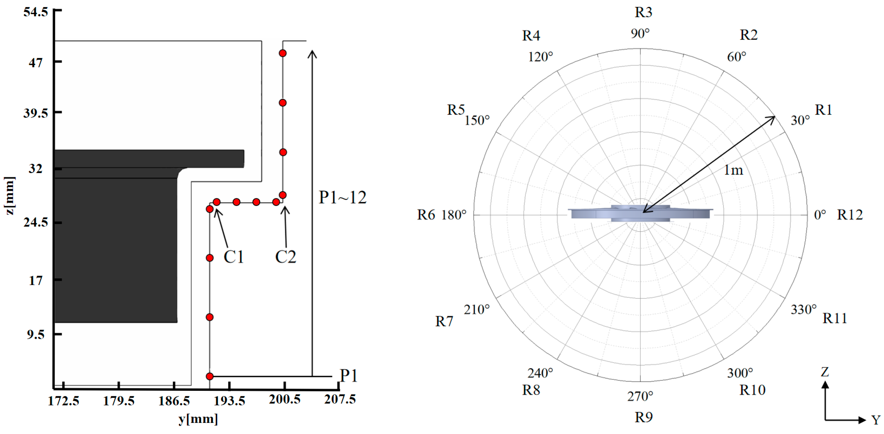
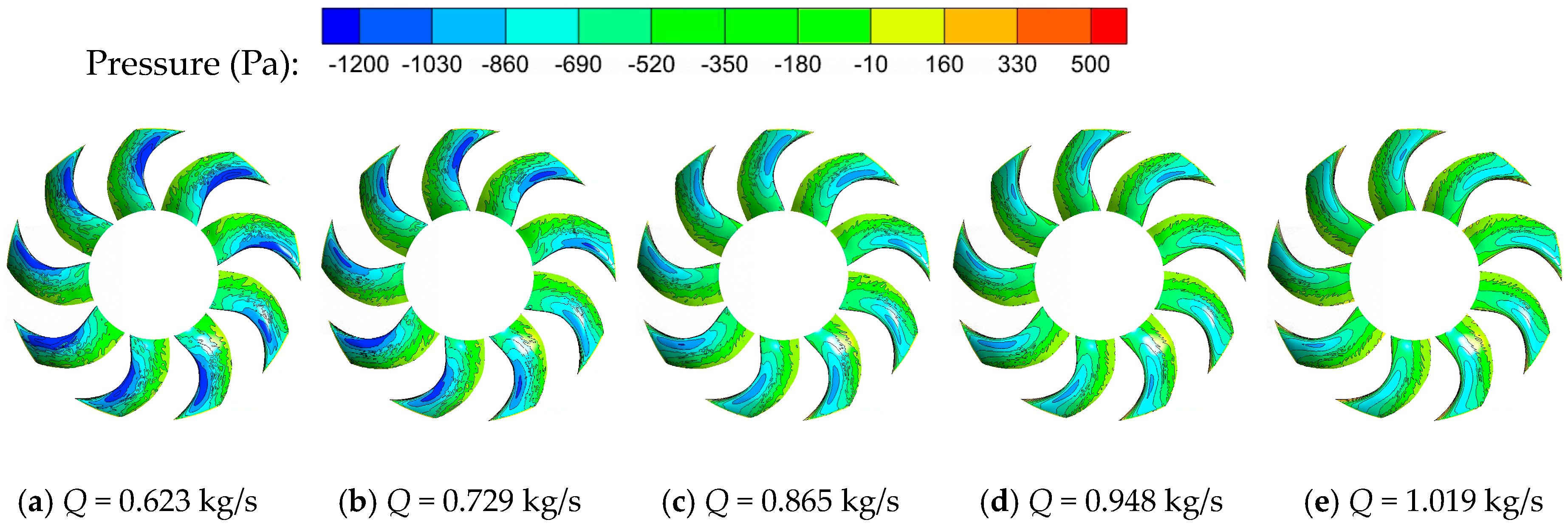
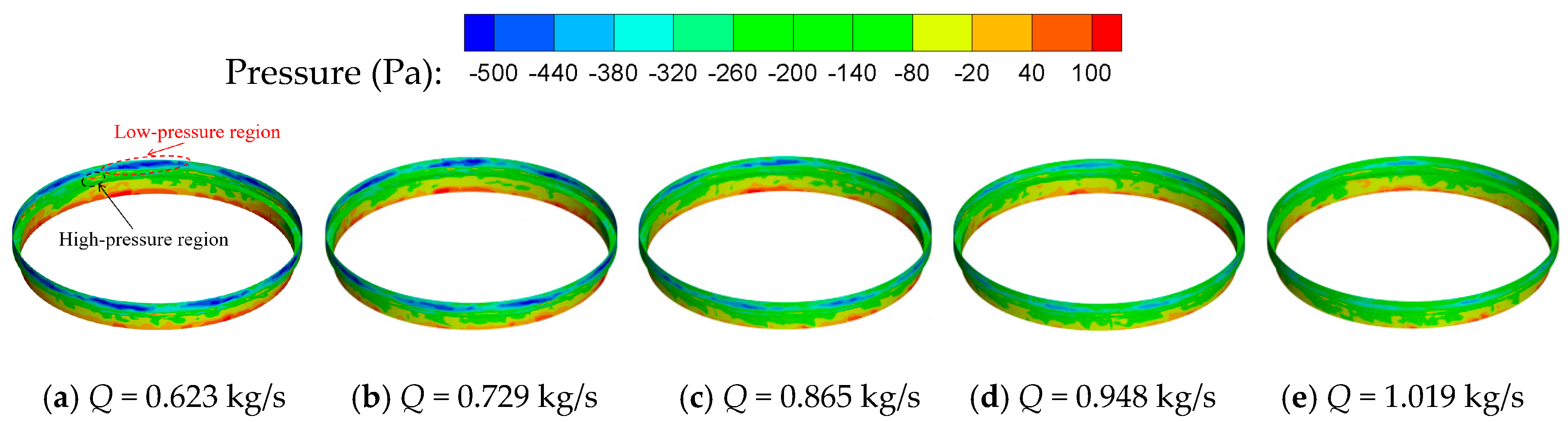
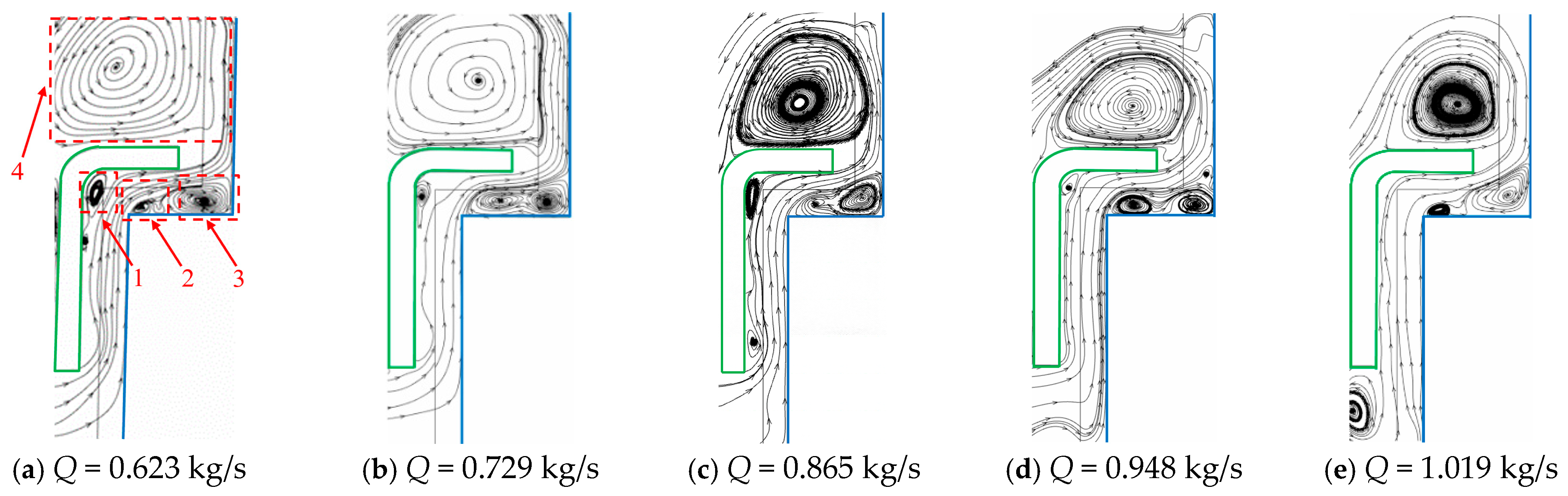
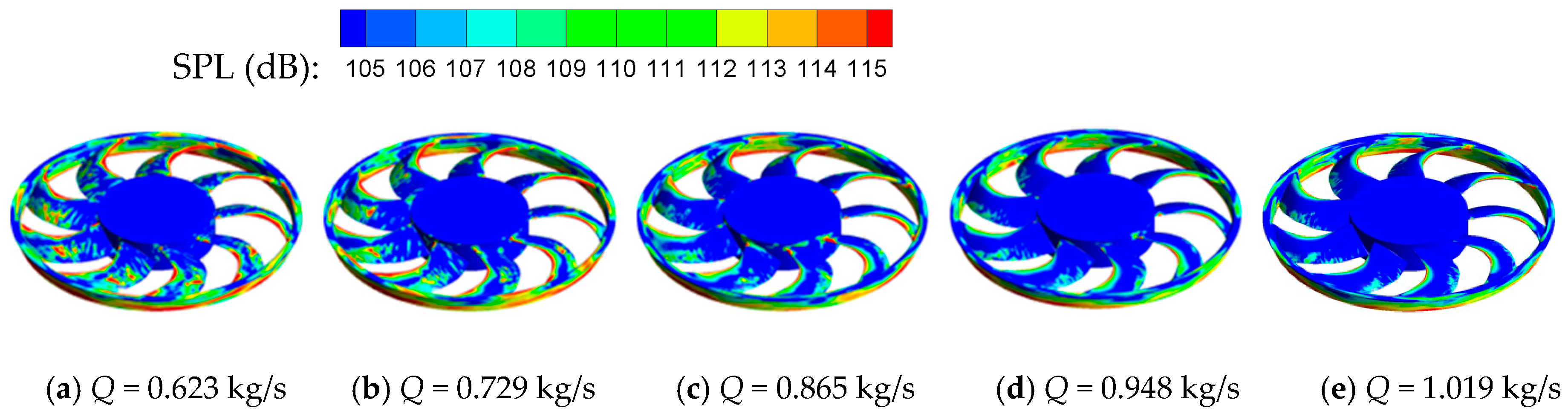
4.1. Aerodynamic Characteristics near the Blade and Shroud

Figure 10 shows the distributions of static pressure in the impeller mid-height plane under different flow rates. It is clearly seen that the evolution trend of static pressure in impeller channels is similar under all flow rates. The static pressure near the pressure surface is significantly higher than that near the suction surface. There is also a low-pressure region near the suction surface at the top of the blade. As the flow rate increases, the static pressure in the impeller basin decreases; the pressure difference in the flow field on either side of the blade also decreases, and the pressure in the low-pressure region near the suction plane at the top of the blade decreases and increases in range.

Figure 11 shows the distributions of static pressure on the suction surface under different flow rates. It can be seen that a low-pressure region exists at the leading edge of the blade and a significant reverse pressure gradient exists on the suction surface. As the flow rate increases, both the low-pressure region and the reverse pressure gradient decrease. This indicates that the flow separation in the leading edge of the blade is weakened. The boundary layer separation on the suction surface is also weakened.

Figure 12 shows the distributions of static pressure on the surface of the shroud under different flow rates. Note, that the static pressure from bottom to top is gradually decreasing on the whole. The maximum and minimum values are 217.4 Pa and −586.9 Pa at a flow rate of 0.623 kg/s, respectively. The deviation of the two values decreases from 804.3 Pa at 0.623 kg/s to 582.2 Pa at 1.019 kg/s. At the same time, the distributions of static pressure present rich fluctuating details. Firstly, several low-pressure regions are observed on the upper part of the shroud, and their number is the same as the number of blades. Secondly, a few high-pressure regions appear around the corner of the shroud.

Figure 13 shows the distributions of streamlining of the clearance under different flow rates, whose position can be seen in Figure 1. It can be seen that the leakage flow is the reverse flow and generally flows from the bottom to the up. Due to the geometric structures, several large-scale vortices appear at corners at a flow rate of 0.623 kg/s. Firstly, a large-scale vortex, which is named vortex 1, is generated and located at the corner of the ring. Subsequently, two large-scale vortices, named vortex 2 and vortex 3, respectively, are formed at two shroud corners C1 and C2. Lastly, the leakage flow flows out of the clearance and mixes with the mainstream flow, forming vortex 4 on the ring. Due to the opposite direction between the leakage flow and the mainstream flow, the energy of the leakage flow is rapidly lost under the interaction. When the energy of the leakage flow is exhausted, it flows into the impeller together with the main flow.

Although vortexes 2 and 3 are insensitive to the flow rate, vortex l weakens until it is not obvious with the increase in flow rate. Moreover, as the flow rate increases, the influence area of leakage flow on the mainstream flow is negatively correlated with the flow rate. This causes the center of vortex 4 shift toward to the outlet clearance.

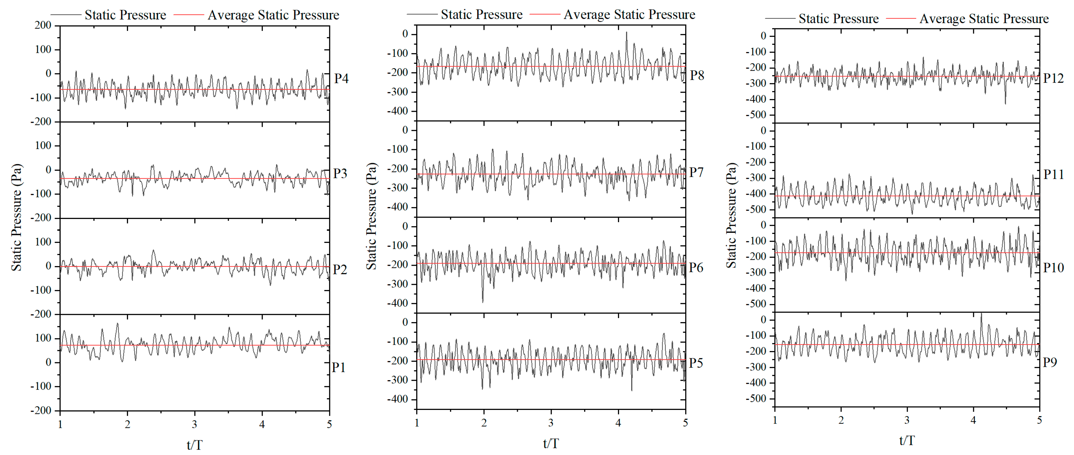
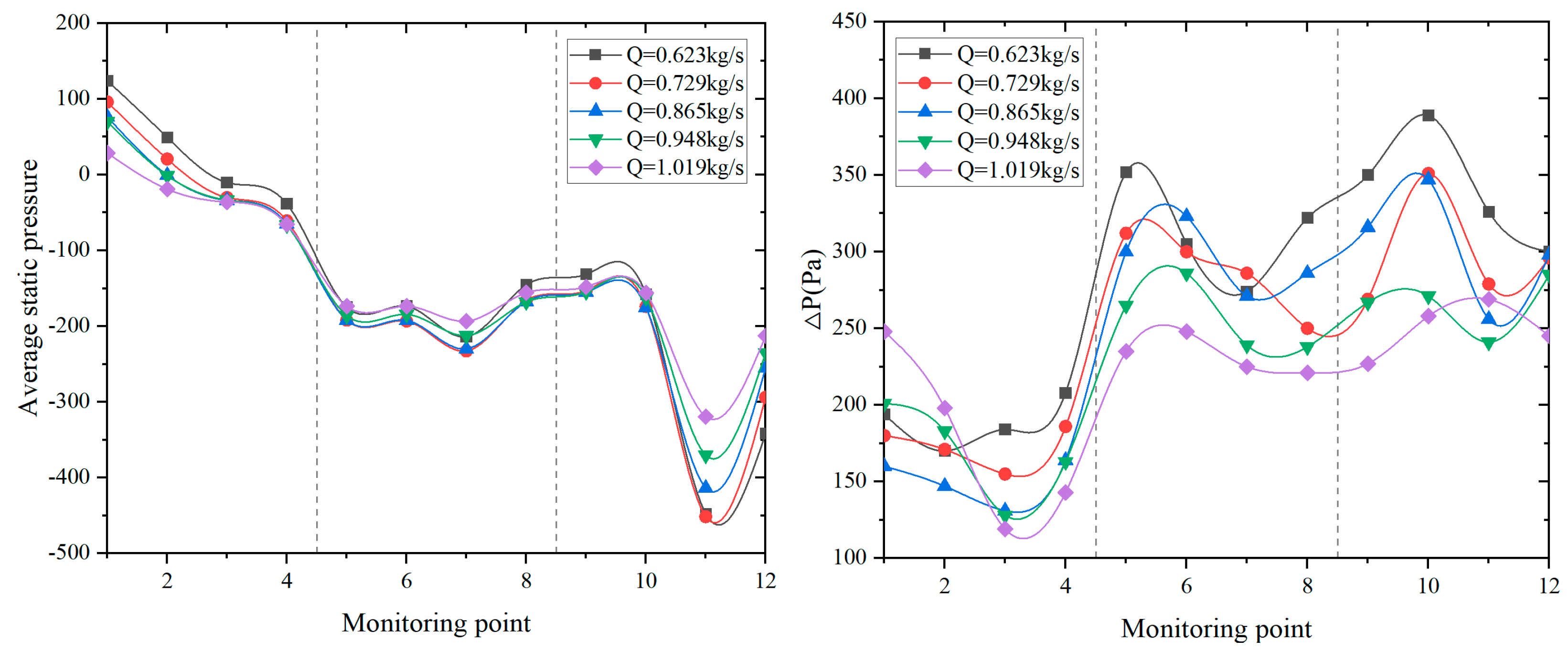
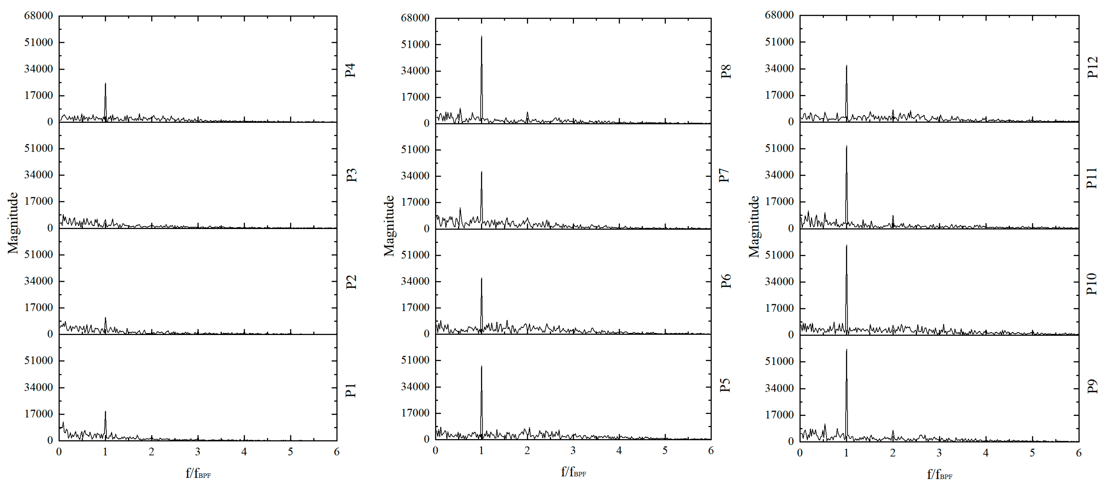
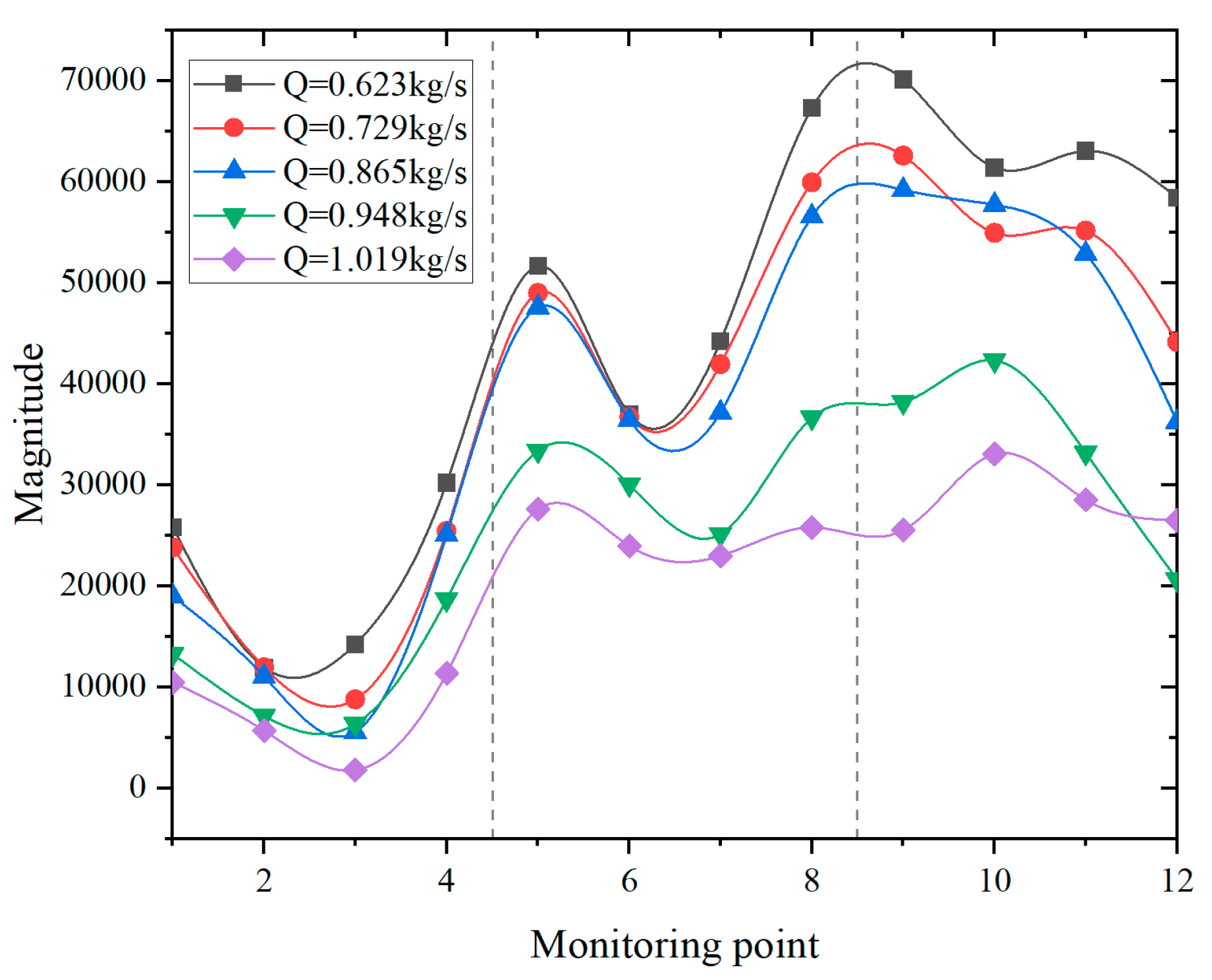
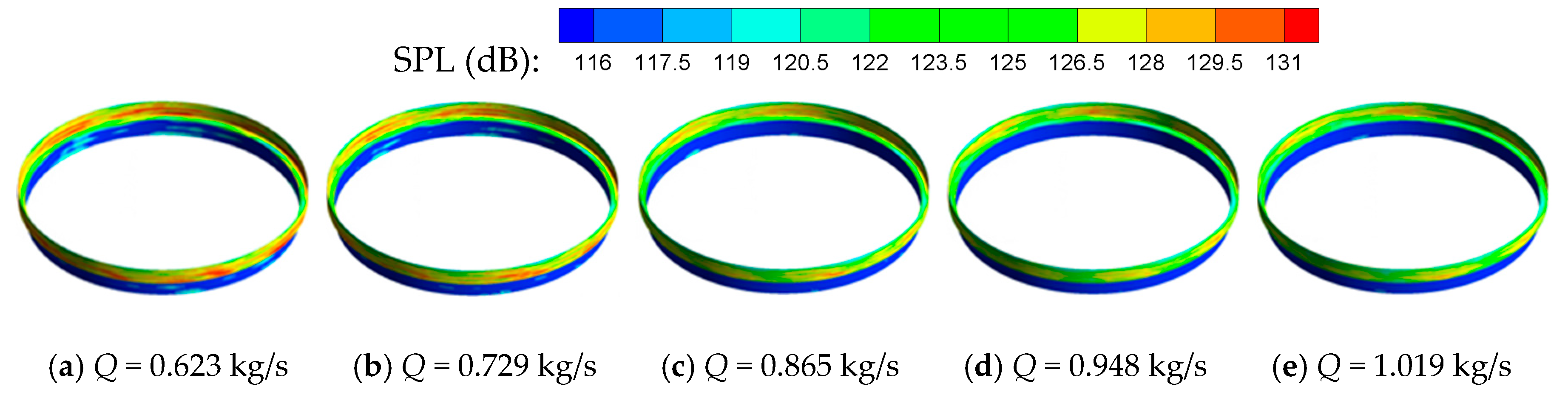
4.2. Pressure Fluctuation near the should

The static pressure fluctuating data during the last four impeller periods are obtained to quantitatively analyze the influence of leakage flow on the pressure at the shroud wall. Figure 14 shows the pressure fluctuations on the shroud wall at 0.865 kg/s. It should be emphasized that there are four monitoring points named for P1 to P4. Firstly, the average static pressure in P1 is 71.8 Pa. With the upward development of the monitoring point, the average static pressure decreases and the value is −65.2 Pa in P4. Secondly, the maximum and minimum values of static pressure in P1 are approximately −163.7 Pa and 3.5 Pa, respectively, indicating that its amplitude is equal to 171.2 Pa. The amplitude of pressure fluctuation first decreases from P1 to P3 and increases at P4. Thirdly, the periodicity of pressure fluctuations in P4 is stronger than that in other monitoring points.

The static pressure fluctuations on the shroud wall of the intermediate section and outlet section are also shown in Figure 14 The average static pressure and the amplitude of pressure fluctuation are obviously smaller and larger than in the inlet section, respectively. Moreover, the periodicity of pressure fluctuations is also significant, which may be related to the large-scale vortex structure.

Figure 15 shows the average static pressure and peak-to-peak value of pressure fluctuation $\Delta P$ under different flow rates. It can be seen that the evolution trend of average static pressure is similar, and its amplitude decreases with increasing flow rates, as shown in Figure 15 (left). The decrease in amplitude is related to the flow rate of the leakage flow. When the pressure difference of the fan decreases with the increase in flow rate, the leakage flow rate decreases due to the decrease in pressure difference in the clearance [34]. An extreme value, $\Delta P$, is observed in each section, including the minimum of the inlet section and the maximum of the other two sections, as shown in Figure 15 (right). As the flow rate increases, the minimum and maximum values decrease. The maximum value of $\Delta P$ in the intermediate section is smaller than that in the outlet section when the flow rate is smaller than 0.865 kg/s. However, an opposite phenomenon is observed when the flow rate is greater than 0.948 kg/s. This is mainly related to flow stability.

Fast Fourier transformation (FFT) is introduced to investigate the pressure frequency characteristics. Figure 16 shows the pressure frequency characteristics of the shroud wall by f/f_BPE at 0.865 kg/s (subscript BPF represents blade passage frequency, and f_BPF = 415 Hz for the cooling fan in the present study). It can be seen that the dominant frequency is independent of monitoring points and is equal to BPF. The amplitude of dominant frequencies in the inlet section is smaller than in the intermediate and outlet sections. The maximum amplitude of the dominant frequency is approximately 59,208.7, which is located at monitoring point P9. This is mainly caused by the large-scale vortex structure.

Figure 17 shows the amplitude of each monitoring point at the BPF in the pressure spectrum under different flow rates. Although the evolution trend of the magnitude of the pressure spectrum is similar, the amplitude decreases as the flow rate increases, especially in the intermediate and outlet sections. Aiming at the condition of the flow rate being less than 0.865 kg/s, the amplitude of the pressure spectrum in the intermediate section is significantly smaller than that in the outlet section. The maximum difference is up to 33,110.3 at 0.623 kg/s. However, this difference is significantly reduced when the flow rate is greater than 0.865 kg/s.

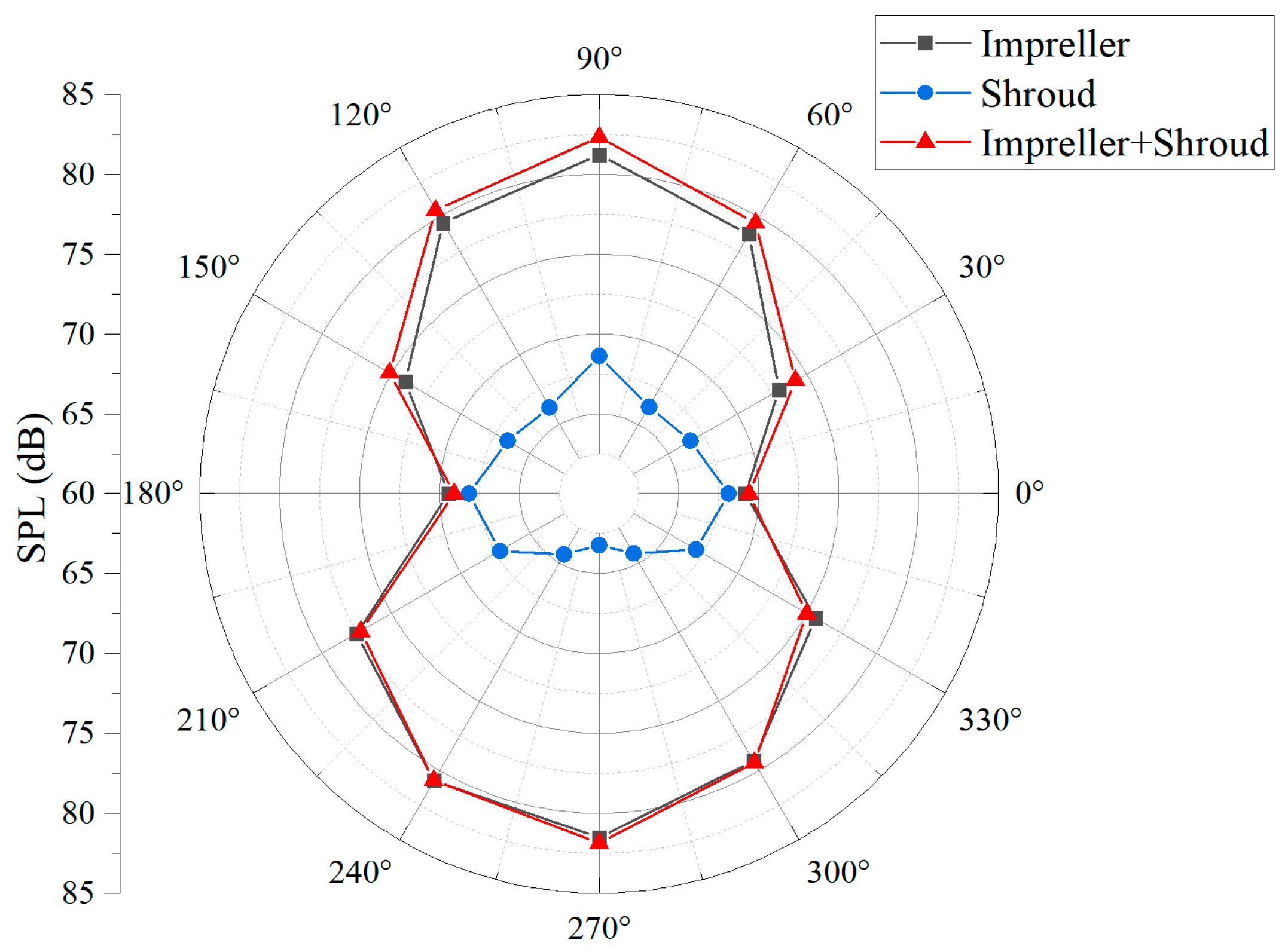
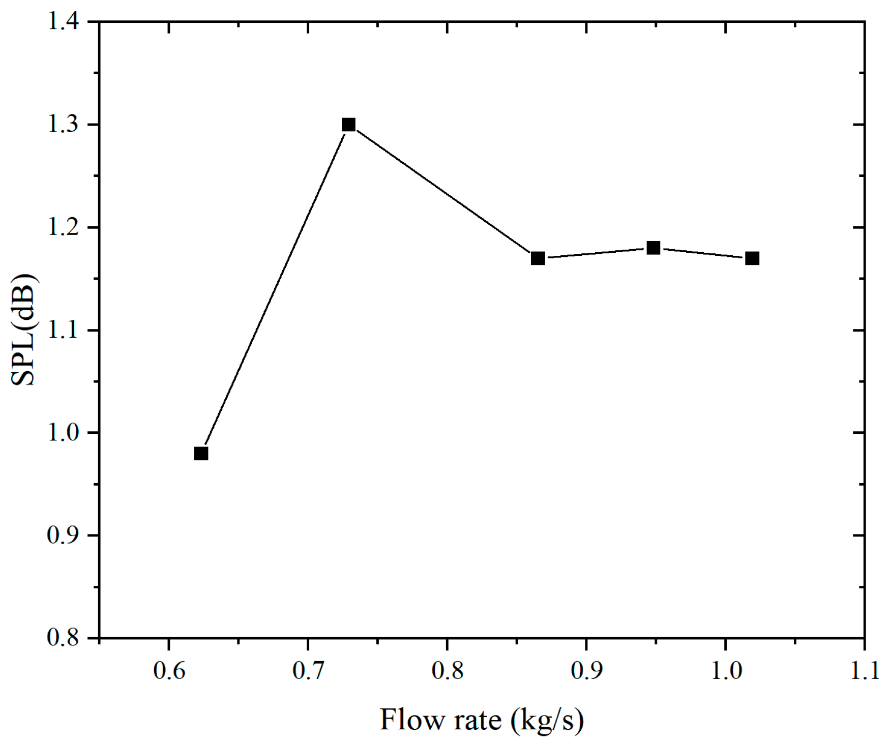
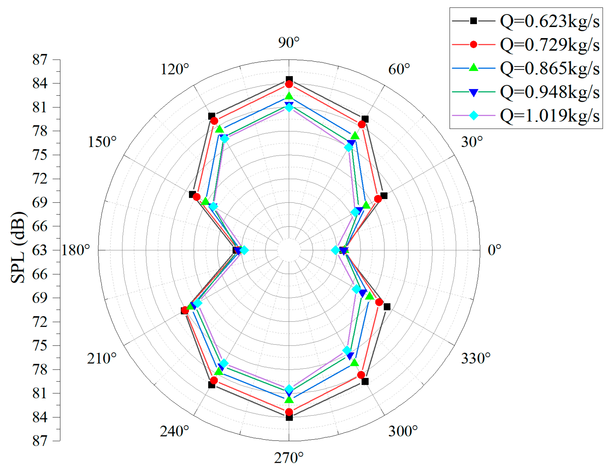
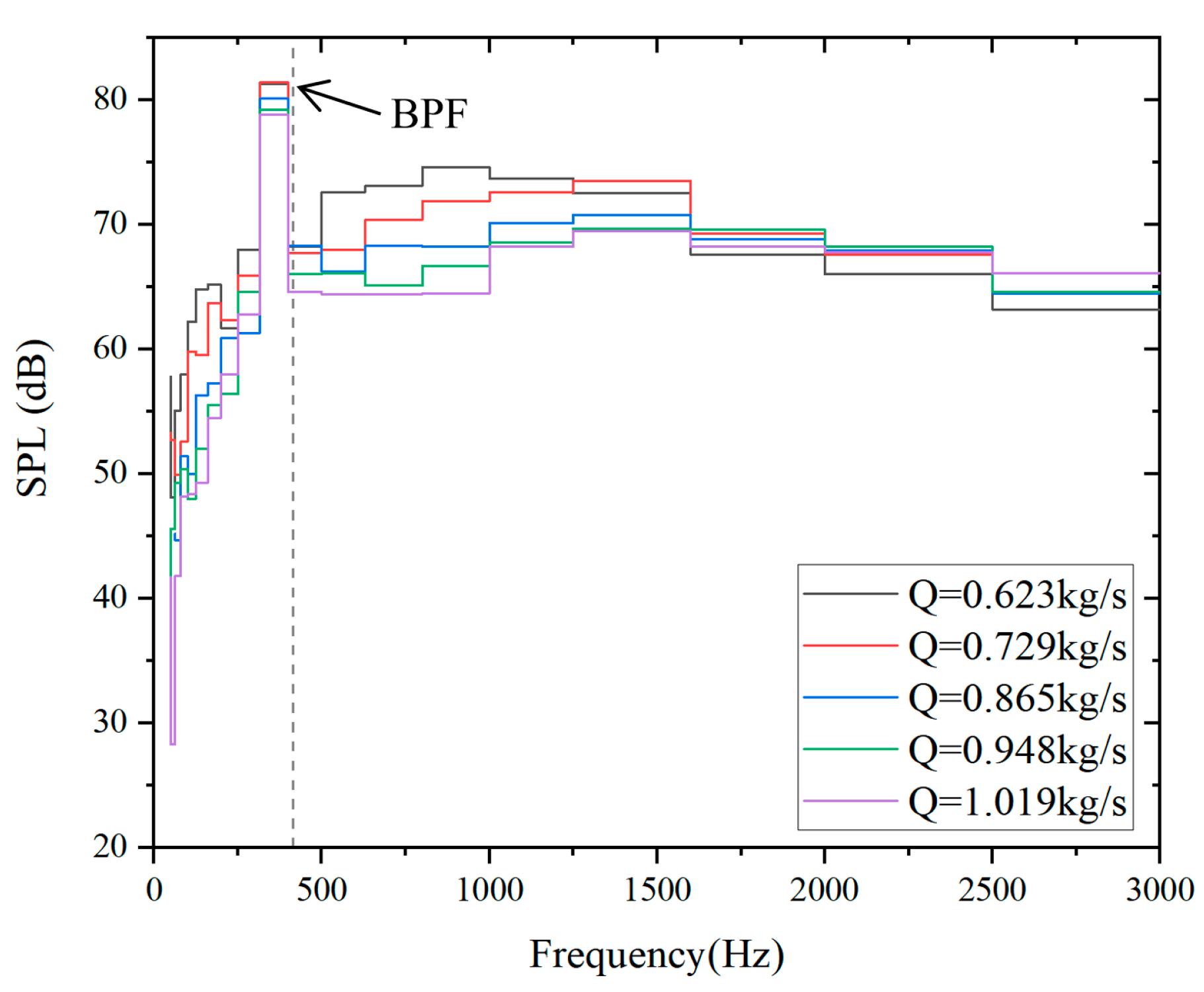
4.3. Aeroacoustic Characteristics

The impeller is one of the important sound source surfaces to induce far-field noise, whose intensity is often expressed by the SPL and defined as follows:

$$\begin{array}{c}{L}_p=20log\frac{P}{P_{ref}}\end{array}$$

(10)

where P is the sound pressure. Subscript “ref” denotes the reference condition. The reference sound pressure is 2 × 10⁻⁵ Pa. Figure 18 shows the far-field noise directivity for three different sound source surfaces at 0.865 kg/s. When the impeller is considered as a sound source surface, a distinct dipole sound source characteristic can be observed. The SPL is larger than 70 dB at most receivers, except R6 and R12. The maximum value of the SPL is 80.69 dB and is located at R9.

When the shroud is considered as a sound source surface, the SPL is relatively small and the distributions of the SPL are significantly different, as shown in Figure 18. The maximum and minimum values of the SPL are located at the fan inlet and at the fan outlet, resulting in a greater contribution to the overall SPL in the fan inlet. Thus, the maximum value of the SPL is 81.86 dB and is located at R3. When the impeller and shroud are both used as sound source surfaces, the change in the SPL at R1 is the largest, with an increase of 1.17 dB.

Figure 19 shows the spectrum of the 1/3 octave band of noise obtained at 0.865 kg/s. Although the SPL at monitor-R1 and monitor-R3 evolved similarly with frequency, the SPL of the former is smaller than that of the latter for all frequency regimes. Considering that the BPF of the impeller is 415 Hz, for all noise sources, the SPL of both monitors near the BPF is significantly higher than other frequencies. This indicates that it has the greatest impact on the overall SPL of the fan. In the low-frequency regime, the SPL shows a rapid increase trend, while in the high-frequency regime, the SPL slowly decreases. At the same time, the shroud has a certain contribution to the magnitude of the SPL for all frequency regimes. Such a contribution in the BPF is approximately 2.1 dB at monitor-Rl and 1.2 dB at monitor-R3.

The contributions of the shroud to the SPL under different flow rates are also investigated, as shown in Figure 20. The maximum deviation of SPL, whose sound source surface with or without shroud, is 1.3 dB.

Figure 21 shows the distribution of the SPL under different flow rates, whose sound source surface is considered impeller and shroud. It can be seen that the distribution trend of the SPL is similar under different flow rates. The SPL decreases as the flow rate increases. The maximum value of the SPL decreases from 84.5 dB at 0.623 kg/s to 80.97 dB at 1.019 kg/s, and the location still occurs at R3.

Figure 22 shows the spectrum of the 1/3 octave band of noise at monitor-R3 under different flow rates; the sound source surface is considered to be the impeller and shroud. The fan model at lower flow rates has a higher magnitude of SPL roughly for the low-frequency regime, while in the high-frequency regime, the fan at higher flow rates has a higher SPL. The maximum SPL is around the frequency of BPF for all flow rates, indicating that it is independent of the flow rates. The maximum deviation is approximately 1.3 dB.

The SPL is highest near the BPF, which contributes most to the overall SPL of the fan. In order to fractionate the main noise sources in this frequency band, the SPL distribution on the impeller surface under different flow rates from 410 HZ to 420 HZ band range is extracted, as shown in Figure 23. It can be seen that the noise of the impeller is mainly concentrated on the blades. The maximum value appears at the leading edge of the blade and reaches a maximum value of 126.3 dB when the flow rate is 0.623 kg/s. Mo et al. [10] also found this phenomenon in an axial cooling fan. This is caused by the flow separation in the leading edge of the blade. As the flow rate increases, the maximum value decreases to 122.8 dB at 1.019 kg/s. This is related to the weakening of the flow separation on the leading edge of the blade with an increasing flow rate. Moreover, a significant decrease in sound pressure level is also found on the suction surface of the blade, which is mainly related to the weakening of the boundary layer separation.

Figure 24 shows the SPL visualization of the shroud noise source between the 410 Hz and 420 Hz band range under different flow rates. The noise on the surface of the shroud is mainly concentrated in the intermediate section and the outlet section. This is consistent with the distribution pattern in Figure 18, with both having higher SPLs in the direction close to the fan inlet. A number of high SPL regions are found near corner C2. These high SPL areas correspond to the location of Vortex 3, indicating that the pressure fluctuations generated by Vortex 3 are the main source of noise generated by the shroud. As the flow rate increases, the pressure fluctuation generated by Vortex 3 weakens. The highest SPL on the surface of the shroud decreased from 130.61 dB at 0.623 kg/s to 128.13 dB at 1.019 kg/s.

5. Conclusions

A numerical investigation on the aerodynamics and aeroacoustics of a cooling fan with a shroud for new energy vehicles and to study the flow rate effects was conducted. The five flow rates range from 0.623 kg/s to 1.019 kg/s; the best efficiency point is 0.865 kg/s. The reliability of the numerical simulation is verified by the grid independence first and then compared with the experimental data, which are obtained from the wind tunnel laboratory of Zhejiang Yinlun Machinery Co. The relative error of static pressure between the numerical simulation and the experimental data verifies the accuracy of the numerical simulation.

The distributions of the static pressure on the shroud surface are more abundant than that in the impeller passage. Strong leakage flow occurs in the clearance between the impeller and the shroud. Due to the geometric structures, several large-scale vortex structures are observed near the shroud corner and clearance outlet. As the flow rate increases, the area of influence of the leakage flow on the mainstream flow decreases.

Regarding the pressure fluctuations near the shroud, the evolution trend of average static pressure is similar at different flow rates, and its amplitude decreases with increasing flow rates. A maximum value of the peak-to-peak values of pressure fluctuations will be found in both the intermediate and outlet sections. The value of the former is smaller than that of the latter at low flow rates, and an opposite phenomenon is observed at high flow rates. The dominant frequency of the pressure spectrum is equal to the BPF, which is independent of the monitoring point and the flow rate. The amplitude of the dominant frequency decreases as the flow rate increases; its position is related to the larger-scale vortex structure.

Although the shroud contributes relatively less to the far-field noise, its different distribution may change the position of the largest SPL. The trend of the SPL is similar under different flow rates, and its maximum value is around the frequency of BPF and is independent of the flow rate. The maximum SPL decreases as the flow rate increases. In addition, the larger SPL is mainly concentrated at the leading edge of the blade and near the corner C2 of the shroud.

The strong turbulence on the surface of the shroud makes the shroud an important sound source surface. Therefore, when considering the noise of the cooling fan, in addition to the impeller, the noise of the shroud should also be considered. In the future, we will conduct a more comprehensive investigation of the aerodynamics and aeroacoustics of a cooling fan with a shroud.

References

1. Suzuki, A.; Soya, A. Study on the Fan Noise Reduction for Automotive Radiator Cooling Fans; SAE Technical Paper; SAE International: Warrendale, PA, USA, 2005. [Google Scholar] [CrossRef]
2. Teymourpour, S.; Mahdavi-Vala, A.; Yadegari, M.; Kia, S.; Seydi, M.; Saboohi, Z. Engineering Approach for Noise Reduction for Automotive Radiator Cooling Fan: A Case Study; SAE Technical Paper; SAE International: Warrendale, PA, USA, 2020. [Google Scholar] [CrossRef]
3. Nashimoto, A.; Fujisawa, N.; Nakano, T.; Yoda, T. Visualization of aerodynamic noise source around a rotating fan blade. J. Vis. 2008, 11, 365–373. [Google Scholar] [CrossRef]
4. Becher, M.; Krusche, R.; Tautz, M.; Mauß, M.; Springer, N.; Krömer, F.; Becker, S. Influence of the gap flow of axial vehicle cooling fans on radiated narrowband and broadband noise. Acta Acust. United Acust. 2019, 105, 435–448. [Google Scholar] [CrossRef]
5. Luo, B.; Chu, W.; Zhang, H. Tip leakage flow and aeroacoustics analysis of a low-speed axial fan. Aerosp. Sci. Technol. 2020, 98, 105700. [Google Scholar] [CrossRef]
6. Zhao, W.; Wasala, S.; Persoons, T. On the Fast Prediction of the Aerodynamic Performance of Electronics Cooling Fans Considering the Effect of Tip Clearance. IEEE Trans. Compon. Packag. Manuf. Technol. 2023, 13, 1139–1146. [Google Scholar] [CrossRef]
7. Park, M.J.; Lee, D.J.; Lee, H. Experimental and computational investigation of the effect of blade sweep on acoustic characteristics of axial fan. Appl. Acoust. 2022, 189, 108613. [Google Scholar] [CrossRef]
8. Azzam, T.; Paridaens, R.; Ravelet, F.; Khelladi, S.; Oualli, H.; Bakir, F. Experimental investigation of an actively controlled automotive cooling fan using steady air injection in the leakage gap. Proc. Inst. Mech. Eng. Part A J. Power Energy 2017, 231, 59–67. [Google Scholar] [CrossRef]
9. Fares, O.; Weng, C.; Zackrisson, L.; Yao, H.; Knutsson, M. Numerical Investigation of Narrow-Band Noise Generation by Automotive Cooling Fans; SAE Technical Paper; SAE International: Warrendale, PA, USA, 2020. [Google Scholar] [CrossRef]
10. Mo, J.; Choi, J. Numerical investigation of unsteady flow and aerodynamic noise characteristics of an automotive axial cooling fan. Appl. Sci. 2020, 10, 5432. [Google Scholar] [CrossRef]
11. Wang, S.; Yu, X.; Shen, L.; Yang, A.; Chen, E.; Fieldhouse, J.; Barton, D.; Kosarieh, S. Noise reduction of automobile cooling fan based on bio-inspired design. Proc. Inst. Mech. Eng. Part D J. Automob. Eng. 2021, 235, 465–478. [Google Scholar] [CrossRef]
12. Park, M.J.; Lee, D.J. Sources of broadband noise of an automotive cooling fan. Appl. Acoust. 2017, 118, 66–75. [Google Scholar] [CrossRef]
13. Moreau, S. Direct noise computation of low-speed ring fans. Acta Acust. United Acust. 2019, 105, 30–42. [Google Scholar] [CrossRef]
14. Chai, P.; Sun, Z.; Chang, Z.; Peng, Z.; Tian, J.; Ouyang, H. Noise characteristics of automobile cooling fan based on circumferential mode analysis. J. Eng. Gas Turbines Power 2021, 143, 121003. [Google Scholar] [CrossRef]
15. Ren, K.; Zhang, S.; Zhang, H.; Deng, C.; Sun, H. Flow field analysis and noise characteristics of an automotive cooling fan at different speeds. Front. Energy Res. 2023, 11, 1259052. [Google Scholar] [CrossRef]
16. Lim, T.G.; Jeon, W.H.; Minorikawa, G. Characteristics of unsteady flow field and flow-induced noise for an axial cooling fan used in a rack mount server computer. J. Mech. Sci. Technol. 2016, 30, 4601–4607. [Google Scholar] [CrossRef]
17. Hu, Z.; Lu, W. Numerical investigation on performance and aerodynamic noise of high speed axial flow fans. In Proceedings of the 2017 IEEE 2nd Advanced Information Technology, Electronic and Automation Control Conference (IAEAC), Chongqing, China, 25–26 March 2017; pp. 885–889. [Google Scholar] [CrossRef]
18. Moosania, M.; Zhou, C.; Hu, S. Aerodynamics of a partial shrouded low-speed axial flow fan. Int. J. Refrig. 2021, 130, 208–216. [Google Scholar] [CrossRef]
19. Canepa, E.; Cattanei, A.; Mazzocut Zecchin, F. Leakage noise and related flow pattern in a low-speed axial fan with rotating shroud. Int. J. Turbomach. Propuls. Power 2019, 4, 17. [Google Scholar] [CrossRef]
20. Daku, G.; Vad, J. Profile vortex shedding from low-speed axial fan rotor blades: A modelling overview. Proc. Inst. Mech. Eng. Part A J. Power Energy 2022, 236, 349–363. [Google Scholar] [CrossRef]
21. Krömer, F.; Müller, J.; Becker, S. Investigation of aeroacoustic properties of low-pressure axial fans with different blade stacking. AIAA J. 2018, 56, 1507–1518. [Google Scholar] [CrossRef]
22. Zhu, T.; Lallier-Daniels, D.; Sanjosé, M.; Moreau, S. Rotating coherent flow structures as a source for narrowband tip clearance noise from axial fans. J. Sound Vib. 2018, 417, 198–215. [Google Scholar] [CrossRef]
23. Eberlinc, M.; Širok, B.; Hočevar, M.; Dular, M. Numerical and experimental investigation of axial fan with trailing edge self-induced blowing. Forsch. Ingenieurwesen 2009, 73, 129–138. [Google Scholar] [CrossRef]
24. Pereira, M.; Ravelet, F.; Azzouz, K.; Azzam, T.; Oualli, H.; Kouidri, S.; Bakir, F. Improved Aerodynamics of a Hollow-Blade Axial Flow Fan by Controlling the Leakage Flow Rate by Air Injection at the Rotating Shroud. Entropy 2021, 23, 877. [Google Scholar] [CrossRef] [PubMed]
25. Ren, G.; Heo, S.; Kim, T.H.; Cheong, C. Response surface method-based optimization of the shroud of an axial cooling fan for high performance and low noise. J. Mech. Sci. Technol. 2013, 27, 33–42. [Google Scholar] [CrossRef]
26. Konikineni, P.; Sundaram, V.; Sathish, K.; Thirukkotti, S. Optimization Solutions for Fan Shroud; SAE Technical Paper; SAE International: Warrendale, PA, USA, 2016. [Google Scholar] [CrossRef]
27. Zhang, X.; Zhang, Y.; Lu, C. Flow and noise characteristics of centrifugal fan in low pressure environment. Processes 2020, 8, 985. [Google Scholar] [CrossRef]
28. Rui, X.; Lin, L.; Wang, J.; Ye, X.; He, H.; Zhang, Z.; Zhu, Z. Experimental and comparative RANS/URANS investigations on the effect of radius of volute tongue on the aerodynamics and aeroacoustics of a sirocco fan. Processes 2020, 8, 1442. [Google Scholar] [CrossRef]
29. Boudet, J.; Cahuzac, A.; Kausche, P.; Jacob, M.C. Zonal large-eddy simulation of a fan tip-clearance flow, with evidence of vortex wandering. J. Turbomach. 2015, 137, 061001. [Google Scholar] [CrossRef]
30. Reboul, G.; Polacsek, C.; Lewy, S.; Heib, S. Aeroacoustic computation of ducted-fan broadband noise using LES data. J. Acoust. Soc. Am. 2008, 123, 3539. [Google Scholar] [CrossRef]
31. Shaheed, R.; Mohammadian, A.; Kheirkhah Gildeh, H. A comparison of standard k–ε and realizable k-ε turbulence models in curved and confluent channels. Environ. Fluid Mech. 2019, 19, 543–568. [Google Scholar] [CrossRef]
32. Lilly, D.K. A proposed modification of the Germano subgrid-scale closure method. Phys. Fluids A Fluid Dyn. 1992, 4, 633–635. [Google Scholar] [CrossRef]
33. Khelladi, S.; Kouidri, S.; Bakir, F.; Rey, R. Predicting tonal noise from a high rotational speed centrifugal fan. J. Sound Vib. 2008, 313, 113–133. [Google Scholar] [CrossRef]
34. Canepa, E.; Cattanei, A.; Moradi, M.; Nilberto, A. Experimental Study of the Leakage Flow in an Axial-Flow Fan at Variable Loading. Int. J. Turbomach. Propuls. Power 2021, 6, 40. [Google Scholar] [CrossRef]
Figure 1. Baseline model of the cooling fan. Front view (left) and section along plane A (right). r1 and r2 equal to 80 mm and 180 mm, respectively.
Processes 12 00333 g001
Figure 2. Layout of monitoring points (left) and acoustic receivers (right).
Processes 12 00333 g002
Figure 3. Three-dimensional computational domains of the cooling fan.
Processes 12 00333 g003
Figure 4. Overall calculation flowchart.
Processes 12 00333 g004
Figure 5. Variation of static pressure rises with grid number of cooling fan domain at flow rate of 0.729 kg/s.
Processes 12 00333 g005
Figure 6. The meshes around the cooling fan (left). The overall fan grid boundary layer grid on the blade (right).
Processes 12 00333 g006
Figure 7. Schematic of the experimental apparatus.
Processes 12 00333 g007
Figure 8. Text fan (left) and wind tunnel test bench (right).
Processes 12 00333 g008
Figure 9. Distributions of static pressure (left) and static pressure efficiency (right).
Processes 12 00333 g009
Figure 10. Distributions of static pressure in the impeller mid-height plane under different flow rates.
Processes 12 00333 g010
Figure 11. Distributions of static pressure on the suction surface under different flow rates.
Processes 12 00333 g011
Figure 12. Distributions of static pressure on the surface of shroud under different flow rates.
Processes 12 00333 g012
Figure 13. Distribution of Streamline in the clearance under different flow rates.
Processes 12 00333 g013
Figure 14. Pressure fluctuations on the shroud wall of inlet section (left), intermediate section (middle) and outlet section (right) at 0.865 kg/s.
Processes 12 00333 g014
Figure 15. Average static pressure (left) and peak-to-peak value of pressure fluctuation (right) under different flow rates.
Processes 12 00333 g015
Figure 16. Pressure spectra on the shroud wall of inlet section (left), intermediate section (middle) and outlet section (right) at 0.865 kg/s.
Processes 12 00333 g016
Figure 17. Amplitude of each monitoring point at BPF in the pressure spectrum under different flow rates.
Processes 12 00333 g017
Figure 18. Far-field noise directivity for three different sound source surfaces at 0.865 kg/s.
Processes 12 00333 g018
Figure 19. Spectrum of 1/3 octave band of noise at R1 (left) and R3 (right) at 0.865 kg/s.
Processes 12 00333 g019
Figure 20. The contributions of shroud to the SPL under different flow rates.
Processes 12 00333 g020
Figure 21. Far-field noise directivity under different flow rates.
Processes 12 00333 g021
Figure 22. Spectrum of 1/3 octave band of noise at R3 under different flow rates.
Processes 12 00333 g022
Figure 23. SPL visualization of the impeller noise source between 410 Hz and 420 Hz band range under different flow rates.
Processes 12 00333 g023
Figure 24. SPL visualization of the shroud noise source between 410 Hz and 420 Hz band range under different flow rates.
Processes 12 00333 g024