Appendix A. Addressing Real-World Conditions Techniques
To effectively model the complex conditions found in industrial environments, this study employs a suite of image processing techniques aimed at replicating the variable lighting and noise interference typically encountered, described analytically in this appendix.
Local brightness fluctuation: This method is designed to emulate localized variations in lighting, akin to the interplay of shadows or spotlights within a scene. Such fluctuations can be indicative of faulty lighting conditions, where certain regions may appear anomalously dark or bright.
where I is the original image, is the modified image, and M is a mask function that applies intensity fluctuations within the specified regions, with representing pixel coordinates.
- 2.
Contrast adjustment in local areas: By locally manipulating the tonal range of the image, this technique can simulate differential light reception across various sections of the image, reflecting the nuanced effects of lighting on the observed subject matter.
where is the contrast adjustment factor, is the mean luminance of the local region, and I and represent the original and modified images, respectively.
- 3.
Dodging and burning: Borrowed from traditional darkroom practices, dodging and burning are digital techniques for selectively brightening (dodging) or darkening (burning) image regions, thus mimicking the variegated effects of light exposure.
For dodging:
For burning:
where
s is the effect strength, and
I and
are the original and modified images.
- 4.
Linear mapping (brightness adjustment): This operation scales the pixel values across the image to adjust brightness, creating the perception that the image was captured under more or less intense light.
where f is the scaling factor for brightness adjustment.
- 5.
Gaussian noise addition: The injection of Gaussian noise into the image serves to replicate the random intensity fluctuations that are often a byproduct of camera sensor noise.
where represents the Gaussian noise function with mean and variance .
- 6.
Multiplicative Gaussian noise: This noise model is proportional to the image intensity, typically used to represent physical phenomena such as speckle in imaging systems.
where denotes the Gaussian noise centered around 1, indicative of no change on average.
Appendix B. Detailed Breakdown of Performance Metrics across All Folds for the Baseline Experiment 1
This appendix contains the detailed breakdown of the performance metrics across all folds, for Experiment 1, summarized in
Section 5.1.
Experiment 1: 5-fold Cross Validation:
Table A1, which details the precision of the model, shows that the model exhibits high precision in identifying crescent gap (Cg) and waist folding (Wf), with scores consistently above 0.94 across all five folds. However, the model struggles with inclusion (In) and silk spot (Ss), where precision is notably lower. This indicates a higher rate of false positives for these defect types.
Table A1.
Precision result of validation in 5-fold cross validation.
Table A1.
Precision result of validation in 5-fold cross validation.
| Defect Types | Fold-1 | Fold-2 | Fold-3 | Fold-4 | Fold-5 |
|---|
| Cr | 0.963 | 0.938 | 0.944 | 0.93 | 0.939 |
| Cg | 0.981 | 0.979 | 0.983 | 0.97 | 0.988 |
| In | 0.602 | 0.648 | 0.688 | 0.578 | 0.532 |
| Os | 0.76 | 0.746 | 0.788 | 0.739 | 0.765 |
| Ph | 0.905 | 0.863 | 0.906 | 0.87 | 0.869 |
| Rp | 0.889 | 0.95 | 0.903 | 0.913 | 0.955 |
| Ss | 0.8 | 0.738 | 0.638 | 0.767 | 0.715 |
| Wf | 0.983 | 0.95 | 0.952 | 0.944 | 0.944 |
| Ws | 0.908 | 0.882 | 0.913 | 0.835 | 0.874 |
| Wl | 0.963 | 0.915 | 0.876 | 0.844 | 0.796 |
| Average | 0.875 | 0.861 | 0.859 | 0.839 | 0.838 |
Table A2 shows the model demonstrates commendable performance in detecting crease (Cr), crescent gap (Cg), and welding line (Wl), with most recall rates being above 0.9. The lower recall rates for inclusion (In) and silk spot (Ss) indicate that the model tends to miss a significant number of these defects, which is a concern for overall detection reliability. The recall rates are slightly lower than precision rates, with averages ranging from 0.796 to 0.835, pointing to a potential area for improvement in the model’s ability to detect all relevant instances.
Table A2.
Recall result of validation in 5-fold cross validation.
Table A2.
Recall result of validation in 5-fold cross validation.
| Defect Types | Fold-1 | Fold-2 | Fold-3 | Fold-4 | Fold-5 |
|---|
| Cr | 0.972 | 0.922 | 0.932 | 0.9 | 0.924 |
| Cg | 0.963 | 0.942 | 0.949 | 0.975 | 0.966 |
| In | 0.651 | 0.599 | 0.656 | 0.561 | 0.519 |
| Os | 0.717 | 0.698 | 0.715 | 0.684 | 0.693 |
| Ph | 0.793 | 0.826 | 0.879 | 0.824 | 0.839 |
| Rp | 0.891 | 0.928 | 0.986 | 0.94 | 0.887 |
| Ss | 0.571 | 0.601 | 0.535 | 0.549 | 0.519 |
| Wf | 0.892 | 0.85 | 0.877 | 0.859 | 0.853 |
| Ws | 0.874 | 0.878 | 0.873 | 0.845 | 0.839 |
| Wl | 0.953 | 0.925 | 0.951 | 0.938 | 0.925 |
| Average | 0.828 | 0.817 | 0.835 | 0.808 | 0.796 |
The F1 score results in
Table A3 demonstrate strong performance in detecting crescent gap (Cg) and waist folding (Wf), with F1 scores consistently high across all folds, particularly notable for Cg with scores above 0.96. In contrast, the model struggles with inclusion (In) and silk spot (Ss), indicated by their notably lower F1 scores, aligning with the trends observed in precision and recall. Other defect types like crease (Cr), welding line (Wl), oil spot (Os), punching hole (Ph), and rolled pit (Rp) show moderate performance with some variability across folds. The average F1 scores, ranging from 0.816 to 0.851, suggest a relatively consistent performance across different data subsets, though with a slight decline in later folds. This table reinforces the findings from previous tables, highlighting the model’s strengths in certain defect types and underscoring areas needing improvement, particularly for defects where both precision and recall are lower.
Table A3.
F1 score result of validation in 5-fold cross validation.
Table A3.
F1 score result of validation in 5-fold cross validation.
| Defect Types | Fold-1 | Fold-2 | Fold-3 | Fold-4 | Fold-5 |
|---|
| Cr | 0.967 | 0.93 | 0.938 | 0.915 | 0.931 |
| Cg | 0.972 | 0.96 | 0.966 | 0.972 | 0.977 |
| In | 0.626 | 0.623 | 0.672 | 0.569 | 0.525 |
| Os | 0.738 | 0.721 | 0.75 | 0.71 | 0.727 |
| Ph | 0.845 | 0.844 | 0.892 | 0.846 | 0.854 |
| Rp | 0.89 | 0.939 | 0.943 | 0.926 | 0.92 |
| Ss | 0.666 | 0.662 | 0.582 | 0.64 | 0.601 |
| Wf | 0.935 | 0.897 | 0.913 | 0.899 | 0.896 |
| Ws | 0.891 | 0.88 | 0.893 | 0.84 | 0.856 |
| Wl | 0.958 | 0.92 | 0.912 | 0.889 | 0.856 |
| Average | 0.851 | 0.838 | 0.847 | 0.823 | 0.816 |
Table A4 presents the model’s performance in terms of mAP50, which is a crucial metric in object detection. Here, the model again shows high scores in detecting crescent gap (Cg), waist folding (Wf), and welding line (Wl), consistent with the high precision and recall rates observed earlier. The lower mAP50 scores for inclusion (In) and silk spot (Ss) reinforce the challenges faced by the model in accurately identifying these defect types. Notably, the average mAP50 demonstrates consistency from folds 1 to 5, which implies that the model can generalize well across different data samples within the same dataset.
Table A4.
mAP50 result of validation in 5-fold cross validation.
Table A4.
mAP50 result of validation in 5-fold cross validation.
| Defect Types | Fold-1 | Fold-2 | Fold-3 | Fold-4 | Fold-5 |
|---|
| Cr | 0.967 | 0.954 | 0.97 | 0.944 | 0.954 |
| Cg | 0.984 | 0.969 | 0.983 | 0.979 | 0.98 |
| In | 0.601 | 0.613 | 0.696 | 0.571 | 0.478 |
| Os | 0.746 | 0.745 | 0.765 | 0.759 | 0.745 |
| Ph | 0.819 | 0.859 | 0.896 | 0.824 | 0.871 |
| Rp | 0.934 | 0.964 | 0.989 | 0.961 | 0.94 |
| Ss | 0.647 | 0.688 | 0.563 | 0.69 | 0.606 |
| Wf | 0.972 | 0.952 | 0.958 | 0.943 | 0.935 |
| Ws | 0.915 | 0.916 | 0.906 | 0.886 | 0.875 |
| Wl | 0.968 | 0.958 | 0.943 | 0.907 | 0.902 |
| Average | 0.855 | 0.862 | 0.867 | 0.846 | 0.829 |
Table A5 sheds light on the model’s performance across a range of IoU thresholds (mAP50-95). The scores here are generally lower than those for mAP50, reflecting the increased difficulty of maintaining high precision at higher IoU thresholds. The model’s performance on inclusion (In) and silk spot (Ss) is particularly affected at these stricter thresholds, with significantly lower scores. The overall lower mAP50-95 scores across all defect types suggest that the model may struggle to maintain high precision when stricter criteria for defect detection are applied.
Table A5.
mAP50-95 result of validation in 5-fold cross validation.
Table A5.
mAP50-95 result of validation in 5-fold cross validation.
| Defect Types | Fold-1 | Fold-2 | Fold-3 | Fold-4 | Fold-5 |
|---|
| Cr | 0.744 | 0.716 | 0.711 | 0.685 | 0.686 |
| Cg | 0.744 | 0.737 | 0.722 | 0.682 | 0.715 |
| In | 0.274 | 0.236 | 0.287 | 0.241 | 0.194 |
| Os | 0.399 | 0.364 | 0.365 | 0.347 | 0.332 |
| Ph | 0.581 | 0.590 | 0.616 | 0.570 | 0.560 |
| Rp | 0.724 | 0.701 | 0.732 | 0.715 | 0.684 |
| Ss | 0.264 | 0.310 | 0.215 | 0.309 | 0.271 |
| Wf | 0.704 | 0.674 | 0.689 | 0.635 | 0.605 |
| Ws | 0.603 | 0.605 | 0.592 | 0.550 | 0.557 |
| Wl | 0.694 | 0.653 | 0.607 | 0.605 | 0.586 |
| Average | 0.573 | 0.559 | 0.554 | 0.534 | 0.519 |
The analysis of the YOLOv5s model’s performance shows that this model, trained on a substantial dataset of 5760 images, demonstrates significant capabilities in certain aspects, while also highlighting potential limitations that could be addressed for enhanced performance. One of the standout observations is the model’s robust ability to detect specific types of defects, notably crescent gap (Cg) and waist folding (Wf). These defect types consistently show high precision, recall, and F1 scores across all folds in the cross-validation process. Such performance suggests that the model has effectively learned to identify the distinguishing features of these defects, possibly due to their distinct characteristics or adequate representation in the training set. Other defects like crease (Cr) and welding line (Wl) also exhibit commendable detection rates, although they display some variability across different folds.
However, the model faces challenges with certain defects, particularly inclusion (In) and silk spot (Ss). These types consistently score lower across all evaluation metrics, indicating difficulties in accurately detecting them. This could be attributed to the complexity of these defects, their resemblance to non-defective areas, similarities with the background, variability within the class, or difficulty in distinguishing this class from others, or extremely small scale illustrated in
Figure 11. The variable performance with defects like oil spot (Os), punching hole (Ph), and rolled pit (Rp) further suggests that while the model is capable of detecting these defects to a certain extent, there is notable room for improvement.
The consistency in the model’s performance, despite a slight decline in average scores across different folds (especially in F1 scores), indicates a general robustness. This suggests that the model’s effectiveness is not overly sensitive to specific data partitions, a crucial aspect for practical applications. However, the observed variability points to potential differences in the difficulty of detecting certain defects in different data subsets, highlighting the importance of a well-rounded and diverse training dataset. An important insight from this analysis is the need for a balance between precision and recall, which varies across defect types. In some cases, higher precision coupled with lower recall suggests a cautious approach by the model, potentially leading to missed defects. On the other hand, higher recall than precision in certain defects could imply over-identification, resulting in false positives. The model’s lower performance in mAP50-95 compared to mAP50 across defect types is indicative of a decline in accuracy at stricter IoU thresholds. This highlights a need for enhancing the model’s robustness and precision, especially in more challenging detection scenarios.
Figure 1.
Sample images from the GC10-DET dataset with 2 examples of each defect: punching hole, welding line, crescent gap, water spot, oil spot, silk spot, inclusion, rolled pit, crease, waist folding.
Figure 1.
Sample images from the GC10-DET dataset with 2 examples of each defect: punching hole, welding line, crescent gap, water spot, oil spot, silk spot, inclusion, rolled pit, crease, waist folding.
Figure 2.
The flowchart of our framework for bias mitigation in single-class and multi-class detection models.
Figure 2.
The flowchart of our framework for bias mitigation in single-class and multi-class detection models.
Figure 3.
Flowchart for preparing image datasets for experimental use. Attention is paid to co-occurring defects in single and multi-class images, as well as under-represented data. Data augmentations also take place to mimic real-world industrial conditions.
Figure 3.
Flowchart for preparing image datasets for experimental use. Attention is paid to co-occurring defects in single and multi-class images, as well as under-represented data. Data augmentations also take place to mimic real-world industrial conditions.
Figure 4.
Examples of images with (a) a single class and (b) multiple classes of metal defects.
Figure 4.
Examples of images with (a) a single class and (b) multiple classes of metal defects.
Figure 5.
Colors used to represent each class of the GC10-DET dataset.
Figure 5.
Colors used to represent each class of the GC10-DET dataset.
Figure 6.
(a) Distribution of the instances in the entire GC10-DET dataset after data verification and correction, before balancing. (b) Distribution of the instances in Group 1 (Single-class images) after data verification and correction, before balancing. (c) Distribution of the instances in Group 2 (multi-class images) after data verification and correction, before balancing. There is high class-imbalance in both single and multi-class images.
Figure 7.
Instance distribution in GC10-DET after data augmentations for balancing classes. (a) Single-class images can be uniformly balanced. (b) Data balancing for multi-class images requires additional attention to co-occurring and infrequently occurring defects.
Figure 7.
Instance distribution in GC10-DET after data augmentations for balancing classes. (a) Single-class images can be uniformly balanced. (b) Data balancing for multi-class images requires additional attention to co-occurring and infrequently occurring defects.
Figure 8.
Instance distribution in GC10-DET after augmentations addressing real-world conditions for (a) Group 1: single class images. The augmentations directly lead to a balanced dataset. (b) Group 2: multi-class images. The augmentations improve dataset balance but do not lead to a perfectly balanced dataset due to the high variability in the occurrences and co-occurrences of class instances.
Figure 9.
A co-occurrence matrix of different classes labeled in Group 2 (before balancing stage).
Figure 9.
A co-occurrence matrix of different classes labeled in Group 2 (before balancing stage).
Figure 10.
Flowchart of model training and evaluation experiments. Left: Experiment 1 baseline model, with a pre-trained model and fine-tuning using single-class images. Right: Experiment 2, exploring fine-tuning the baseline model using multi-class images.
Figure 10.
Flowchart of model training and evaluation experiments. Left: Experiment 1 baseline model, with a pre-trained model and fine-tuning using single-class images. Right: Experiment 2, exploring fine-tuning the baseline model using multi-class images.
Figure 11.
The yellow box in each image shows different cases of challenging defects (from left to right): Silk spot defect very similar to the background and other classes; Inclusion defects with high intra-class variability, the one on the right also similar to the background and other defect classes; Silk spot defect of an extremely small scale.
Figure 12.
Different colors to represent the different folds in the 5-fold cross validation experiments on generalizability.
Figure 12.
Different colors to represent the different folds in the 5-fold cross validation experiments on generalizability.
Figure 13.
Training (
a) box, (
b) class, (
c) object losses in 5-fold cross validation, with each different color corresponding to a fold as in
Figure 12.
Figure 13.
Training (
a) box, (
b) class, (
c) object losses in 5-fold cross validation, with each different color corresponding to a fold as in
Figure 12.
Figure 14.
Validation (
a) box, (
b) class, (
c) object losses in 5-fold cross validation, with each different color corresponding to a fold as in
Figure 12.
Figure 14.
Validation (
a) box, (
b) class, (
c) object losses in 5-fold cross validation, with each different color corresponding to a fold as in
Figure 12.
Figure 15.
Performance metrics (
a) precision, (
b) recall, (
c) mAP50, (
d) mAP50-95 across 5-fold cross validation, with each different color corresponding to a fold as in
Figure 12.
Figure 15.
Performance metrics (
a) precision, (
b) recall, (
c) mAP50, (
d) mAP50-95 across 5-fold cross validation, with each different color corresponding to a fold as in
Figure 12.
Figure 16.
Evaluation of (
a) precision, (
b) recall, (
c) F1 score of Experiment 2 show the performance for different numbers of frozen layers with colors representing the different classes of
Figure 5.
Figure 16.
Evaluation of (
a) precision, (
b) recall, (
c) F1 score of Experiment 2 show the performance for different numbers of frozen layers with colors representing the different classes of
Figure 5.
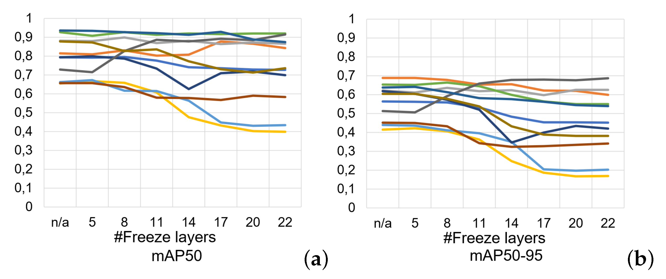
Figure 17.
Evaluation of (
a) mAP50, (
b) mAP50-95 metrics of Experiment 2 show the performance for different numbers of frozen layers with colors representing the different classes of
Figure 5.
Figure 17.
Evaluation of (
a) mAP50, (
b) mAP50-95 metrics of Experiment 2 show the performance for different numbers of frozen layers with colors representing the different classes of
Figure 5.
Figure 18.
Flowchart of training and evaluation. Left: Experiment 3 explores the effect of diverse multi-class training data on generalizability, fairness and bias. Right: Experiment 4 examines the effect of data augmentation on single-class images.
Figure 18.
Flowchart of training and evaluation. Left: Experiment 3 explores the effect of diverse multi-class training data on generalizability, fairness and bias. Right: Experiment 4 examines the effect of data augmentation on single-class images.
Figure 19.
Distribution of instances for metallic surface defect classes in (
a) Experiments 3 and (
b) 4, with the color labels shown in
Figure 5.
Figure 19.
Distribution of instances for metallic surface defect classes in (
a) Experiments 3 and (
b) 4, with the color labels shown in
Figure 5.
Figure 20.
Confusion matrices of Experiments 1–4 (testing set). Experiment 3 has most predictions along its diagonal, showing it most accurately identifies the majority of defects when tested on different types of data, demonstrating its improved generalizability, reduced bias and improved fairness.
Figure 21.
Eigen-CAM results of predicting 2 similar defects in Experiments 1, 2, 3, and 4. The red square shows the captured predicted area and the red arrows denote erroneous predictions. It is clear that the model successfully focuses on the relevant areas of test images for Experiment 3, while these are largely missed by the other experimental setups.
Table 1.
Experimental setup: YOLOv5s fixed hyperparameters.
Table 1.
Experimental setup: YOLOv5s fixed hyperparameters.
| Learning rate | initial: 0.01, final: 0.01 |
| Momentum | 0.937 |
| Weight decay | 0.0005 |
| Warmup epochs | 3 |
| Warmup momentum | 0.8 |
| Warmup bias learning rate | 0.1 |
| Box loss weight | 0.05 |
| Class loss weight | 0.5 |
| Class penalty weight | 1.0 |
| Box loss weight | 0.05 |
| Object loss weight | 1.0 |
| Object penalty weight | 1.0 |
| IOU threshold for objectness | 0.2 |
| Object penalty weight | 1.0 |
| Anchor threshold | 4.0 |
| Focal loss gamma | 0.0 |
Table 2.
Average performance metrics values in 5-fold cross validation: precision, recall, F1 score, mAP50, mAP50-95 all show there is no overfitting.
Table 2.
Average performance metrics values in 5-fold cross validation: precision, recall, F1 score, mAP50, mAP50-95 all show there is no overfitting.
| Defect Types | Fold-1 | Fold-2 | Fold-3 | Fold-4 | Fold-5 |
|---|
| Average Precision | 0.875 | 0.861 | 0.859 | 0.839 | 0.838 |
| Average Recall | 0.828 | 0.817 | 0.835 | 0.808 | 0.796 |
| Average F1 Score | 0.851 | 0.838 | 0.847 | 0.823 | 0.816 |
| Average mAP50 | 0.855 | 0.862 | 0.867 | 0.846 | 0.829 |
| Average mAP50-95 | 0.573 | 0.559 | 0.554 | 0.534 | 0.519 |
Table 3.
Average precision, recall, F1 score of Experiment 1, 2, 3, 4. Experiment 3 consistently outperforms the other experimental setups.
Table 3.
Average precision, recall, F1 score of Experiment 1, 2, 3, 4. Experiment 3 consistently outperforms the other experimental setups.
| | Exp 1 | Exp 2 | Exp 3 | Exp 4 |
|---|
| Average Precision | 0.773 | 0.825 | 0.882 | 0.786 |
| Average Recall | 0.528 | 0.715 | 0.838 | 0.533 |
| Average F1 Score | 0.627 | 0.766 | 0.859 | 0.635 |
Table 4.
Precision of Experiment 1, 2, 3, 4. Experiment 3 outperforms the others for most defect classes.
Table 4.
Precision of Experiment 1, 2, 3, 4. Experiment 3 outperforms the others for most defect classes.
| Defect Types | Exp 1 | Exp 2 | Exp 3 | Exp 4 |
|---|
| Cr | 0.851 | 0.834 | 0.938 | 0.907 |
| Cg | 0.962 | 0.841 | 0.895 | 0.928 |
| In | 0.398 | 0.71 | 0.667 | 0.42 |
| Os | 0.631 | 0.756 | 0.864 | 0.552 |
| Ph | 0.932 | 0.913 | 0.953 | 0.897 |
| Rp | 0.683 | 0.785 | 0.896 | 0.746 |
| Ss | 0.633 | 0.794 | 0.766 | 0.714 |
| Wf | 0.965 | 0.871 | 0.982 | 0.974 |
| Ws | 0.846 | 0.871 | 0.899 | 0.857 |
| Wl | 0.831 | 0.88 | 0.959 | 0.864 |
| Average | 0.773 | 0.825 | 0.882 | 0.786 |
Table 5.
Recall of Experiment 1, 2, 3, 4. Experiment 3 outperforms the others for most defect classes.
Table 5.
Recall of Experiment 1, 2, 3, 4. Experiment 3 outperforms the others for most defect classes.
| Defect Types | Exp 1 | Exp 2 | Exp 3 | Exp 4 |
|---|
| Cr | 0.426 | 0.728 | 0.957 | 0.415 |
| Cg | 0.581 | 0.836 | 0.86 | 0.597 |
| In | 0.393 | 0.584 | 0.703 | 0.37 |
| Os | 0.329 | 0.643 | 0.708 | 0.36 |
| Ph | 0.85 | 0.9 | 0.903 | 0.85 |
| Rp | 0.361 | 0.541 | 0.941 | 0.37 |
| Ss | 0.295 | 0.577 | 0.558 | 0.271 |
| Wf | 0.917 | 0.749 | 0.909 | 0.926 |
| Ws | 0.52 | 0.695 | 0.899 | 0.527 |
| Wl | 0.611 | 0.891 | 0.938 | 0.646 |
| Average | 0.528 | 0.715 | 0.838 | 0.533 |
Table 6.
F1 score of Experiment 1, 2, 3, 4. Experiment 3 outperforms the others for most defect classes.
Table 6.
F1 score of Experiment 1, 2, 3, 4. Experiment 3 outperforms the others for most defect classes.
| Defect Types | Exp 1 | Exp 2 | Exp 3 | Exp 4 |
|---|
| Cr | 0.568 | 0.777 | 0.947 | 0.569 |
| Cg | 0.724 | 0.838 | 0.877 | 0.727 |
| In | 0.395 | 0.641 | 0.685 | 0.393 |
| Os | 0.432 | 0.695 | 0.778 | 0.436 |
| Ph | 0.889 | 0.906 | 0.927 | 0.873 |
| Rp | 0.472 | 0.641 | 0.918 | 0.495 |
| Ss | 0.402 | 0.668 | 0.646 | 0.393 |
| Wf | 0.940 | 0.805 | 0.944 | 0.949 |
| Ws | 0.644 | 0.773 | 0.899 | 0.653 |
| Wl | 0.704 | 0.885 | 0.948 | 0.739 |
| Average | 0.627 | 0.766 | 0.859 | 0.635 |
Table 7.
mAP50 of Experiment 1, 2, 3, 4. Experiment 3 outperforms the others for most defect classes.
Table 7.
mAP50 of Experiment 1, 2, 3, 4. Experiment 3 outperforms the others for most defect classes.
| Defect Types | Exp 1 | Exp 2 | Exp 3 | Exp 4 |
|---|
| Cr | 0.664 | 0.811 | 0.977 | 0.677 |
| Cg | 0.779 | 0.887 | 0.911 | 0.78 |
| In | 0.353 | 0.656 | 0.715 | 0.385 |
| Os | 0.483 | 0.693 | 0.802 | 0.477 |
| Ph | 0.91 | 0.886 | 0.938 | 0.908 |
| Rp | 0.574 | 0.588 | 0.957 | 0.601 |
| Ss | 0.471 | 0.642 | 0.69 | 0.47 |
| Wf | 0.94 | 0.808 | 0.944 | 0.952 |
| Ws | 0.682 | 0.81 | 0.915 | 0.688 |
| Wl | 0.737 | 0.906 | 0.961 | 0.76 |
| Average | 0.659 | 0.769 | 0.881 | 0.67 |
Table 8.
mAP50-95 of Experiment 1, 2, 3, 4. Experiment 3 outperforms the others for most defect classes.
Table 8.
mAP50-95 of Experiment 1, 2, 3, 4. Experiment 3 outperforms the others for most defect classes.
| Defect Types | Exp 1 | Exp 2 | Exp 3 | Exp 4 |
|---|
| Cr | 0.486 | 0.61 | 0.824 | 0.499 |
| Cg | 0.616 | 0.615 | 0.706 | 0.61 |
| In | 0.135 | 0.377 | 0.391 | 0.164 |
| Os | 0.251 | 0.411 | 0.517 | 0.239 |
| Ph | 0.502 | 0.607 | 0.677 | 0.493 |
| Rp | 0.455 | 0.382 | 0.727 | 0.465 |
| Ss | 0.232 | 0.398 | 0.432 | 0.227 |
| Wf | 0.727 | 0.527 | 0.747 | 0.745 |
| Ws | 0.416 | 0.516 | 0.605 | 0.436 |
| Wl | 0.457 | 0.539 | 0.655 | 0.461 |
| Average | 0.428 | 0.498 | 0.628 | 0.434 |
Table 9.
Fairness measures results in Experiments 1, 2, 3, and 4 with the best outcomes shown in bold. Experiment 3 leads to the most fair and unbiased outcomes in all cases, and the same outcome for PPD as Experiment 2.
Table 9.
Fairness measures results in Experiments 1, 2, 3, and 4 with the best outcomes shown in bold. Experiment 3 leads to the most fair and unbiased outcomes in all cases, and the same outcome for PPD as Experiment 2.
| Experiments | DIR | TPR Diff. | PP Diff. |
|---|
| 1 | 1.52 | 0.24 | −0.19 |
| 2 | 1.39 | 0.26 | −0.08 |
| 3 | 1.14 | 0.11 | −0.08 |
| 4 | 1.56 | 0.26 | −0.17 |


