A Numerical Study on the Performance of a Pumping Station with Bell-Mouth-Based Vertical Pumps during an Accidental Shutdown

Abstract

This study presents a numerical simulation of a pump’s performance during a power-cut event and connected hazards resulting from the failure of non-return flap valves. The vertical mixed-flow pumps with suction bells were mounted inside the suction basins of a pumping station. Different regimes of the pump operation during the time were analyzed based on the pump’s 4-quadrant characteristics and the dynamics of rotating parts in the pump, gearbox and electric engine. The resulting development of flow rates, rotor speed and forces in the course of time were used to analyze the hazards of failure of any pumping system component and the flooding of the suction object and its surroundings. The presented results show a deep insight into the flow phenomena in vertical mixed-flow pumps with suction bells during the runaway process and confirm that the developed methodology can be successfully applied to monitor the critical regimes in a pumping station in real time. The simulations were verified with some experimentally obtained data.

1. Introduction

This article focuses on the abnormal operation of a pumping station, which represents a complete hydraulic system equipped with several pumps, connecting piping and the suction and discharge objects. The analysis is based on the numerical simulation of multiphase flow with the free water level.

Ordinarily, the suction objects are equipped with the draft tubes, to which the pumps are connected, or in the case of the application of vertical pumps, the open sump intake design is applied, in which the pumps are equipped with some form of suction bells. In this study, the vertical mixed-flow pumps with the suction bells are mounted inside the intake objects with a free level and separated with the concrete walls. There are many experimental and numerical studies concerning the free-surface flows close to the pump sump with such an arrangement during the pumping regime. First of all, the operation of pumps is very sensitive to the vortical structures entering the impeller. In the case of vertical pumps with the suction bells, both the free surface vortices and the submerged vortices can be often observed as a result of the pressure drop and the pre-rotation flow in the vicinity of the pump suction. They cause many unwanted effects as the unsteady nonuniform flow resulting in the impeller vibrations or the cavitation effects in the vortex core. The free surface vortices are particularly undesirable, as they can cause the danger of air entrainment from the free surface. Increasing the submergence value is a typical way to avoid these vortices because they are directly related to the submergence value. Anti-Vortex Devices (AVDs) are frequently used to suppress both the free surface vortices and the submerged vortices [1,2]; they can significantly decrease the angular momentum of flow. It is very important to predict the operation conditions when the above-mentioned phenomena take place and then to prevent their formation. That is why these phenomena are widely examined both numerically and experimentally [3,4,5,6,7,8,9,10,11]. Due to the time and financial costs, Computational Fluid Dynamics (CFD) methods prevail. Most of the available studies are devoted to the pumping regime, but there are practically no studies linked to the turbine or abnormal regimes, especially in the case of the vertical pumps with suction bells and the presence of AVD.

Though the discharge objects are less important in this study, they are included in the case description. Two hydraulic designs of the discharge are considered, as they are favored for safety reasons and can be easily installed and operated, with minimum mechanical and electronic equipment. The first solution is based on the overflow walls, and the second one is based on the siphon outlets. According to the authors’ knowledge, there are few works dealing with the numerical simulations of the supercritical and especially near-critical flows over the overflow walls. Interesting results can be found, e.g., in [12,13,14,15], considering the broad-crested and sharp-crested weirs with a 2D geometry, or [13] considering the side weir. The modeling of a complete pump station with a V-shaped broad-crested weir can be found in [16]. Compared to the overflow walls, siphons offer a possibly higher hydraulic efficiency, but a siphon-breaking valve is required to prevent back-flow and allow for venting at start-up. Numerical simulations of a complete pumping system with the siphon outlet, modeling the flow as the single-phase one, are presented in [17]. The complex models, also considering the free water level, can be found in [18], where the transient phenomena during the stopping process in the axial-flow pump system with the siphon outlet are simulated, or in [15], which models the transient phenomena during the start-up phase of the complete pumping station with the welded siphon. A combined experimental and numerical research of the siphon flow applying both the CFD tools and the lattice-Boltzmann method is described in [19,20]. The numerical simulations considering the multiphase flow with the free water level commonly use the VOF (Volume of Fluid) model [21]. This multiphase flow model solves the equation for the volume fraction of the liquid component and does not take into account the formation of individual water particles or air and water vapor bubbles and their interactions.

After the pump is accidentally switched off or the electric power is lost due to the failure and the (possibly existing) valve fails, both in the case of overflow walls and the siphon discharge, the water gradually stops to flow up and due to the gravity forces starts to flow back to empty the discharge piping. This may not be a serious problem when a short discharge piping contains a small, limited amount of water. But in the case of the discharge piping with the diameter in meters and length in kilometers, a large amount of water returns back to the suction basin with the serious water waves and flooding capacity. Also, the time necessary to empty the discharge piping can be very long. During this process, the pump gradually changes its operation regime from the pump one (when the pumped water flows inside the pump from its suction side to the discharge piping while the pump shaft rotates in the pump direction) to the no-load turbine conditions when the water flows from the discharge piping to the pump suction while the pump shaft rotates close to the turbine runaway speed. During this time span, the brake regime has to be considered when the pumped water flows inside the pump from its discharge piping to the suction side while the pump shaft rotates in the pump direction. The achieved shaft speed is very important for the pump, the gear box and the motor and its cooling. Also, the achieved flow rates are important to design the suction basin and its surroundings.

To be able to analyze the pump performance during the accidental shutdown, a large part of the full 4-quadrant behavior must be known, typically in the form of the dimensionless variables. The advantage of the creation of a dimensionless representation of the 4-quadrant characteristics is a possibility of repeated calculations for different cases and initial states, without the necessity of repeated CFD simulations, which are very expensive and CPU-time-consuming. On the other hand, using the 4-quadrant characteristics, one must rely on the validity of the hydraulic affinity laws and should be careful of their range. There are many references related to the 4-quadrant characteristics, with the classical form of the dimensionless variables [22,23,24,25] or with different modifications, e.g., in the form of the Suter curves [26]. Also, the range of utilization of the 4-quadrant characteristics is very broad in PAT (Pump as Turbine) applications, from the PAT turbine startup [27,28,29], through the pump–turbine transition [30,31], up to the “S” zone close to the turbine runaway conditions, where the so-called S-instability occurs [32,33,34,35,36,37]. The simulation of pump performance during the accidental shutdown can be found, e.g., in [38], where a large vertical mixed-flow pump with a draft tube is modeled inside the commercial CFD software ANSYS Fluent with the angular momentum acting on the impeller updated in each time step by a User-Defined Function (UDF), or in [39], where the runaway and runaway shutdown processes of the tubular turbine inside the circulating cooling water system are simulated based on the combination of CFD and the method of characteristics (MOC) and also using the Fluent UDF. The process of power failure in the case of the submersible tubular pump is also solved in [40] using the direct combination of the Fluent code and the 6DOF model based on the fourth-order multi-point Adams–Moulton formula. Numerical simulations of the bidirectional transition from the pump to turbine modes and back can be found in [41], where, in the process of a transient simulation, the torque balance equation is applied for calculating the rotational speed of the impeller through the Fluent UDF.

References dealing with the S-instability mentioned above indicate a close relation of this instability to the complex pattern of vortical structures appearing especially inside the runner. A detailed analysis of the vortex evolution in the runner of a PAT under the runaway conditions combined with an experimental verification can be found in [42], while in [43], an advanced experimental research on flow fields inside the pump–turbine by means of the Particle Imaging Velocimetry (PIV) is presented in combination with the full-flow numerical simulation. The Delayed Detached-Eddy Simulation (DDES) is applied in [44] to the analysis of the transient vortices in the runner and the draft tube of a PAT during the S-instability. All these studies confirm very unfavorable flow conditions linked with the S-shaped curve. The complexity of the flow conditions can even be increased by the presence of the free water level. A detailed view of complex vortical structures interacting with the free water level inside a very low head (VLH) turbine in an open channel under no-load conditions can be found in [45].

As it has been already mentioned at the beginning of this section, the aim of this paper is to describe the abnormal situation of when the pump trip appears, but the paper also aims to present a methodology which can be successfully applied to monitor various critical regimes in the pumping station in real time. Against the above background, the paper is composed as follows. Section 2 presents, in detail, the study case and the methods used within the CFD analysis and the 1D dynamic model. Section 3 shows key differences in the flow fields during the most important operating modes of the pumps, equipped with the suction bells and AVD, derived complete 4-quadrant characteristics and the results of the simulation of the station power cut event. The obtained data and the applicability of the presented methodology are discussed in the Discussion and Conclusions sections.

2. Materials and Methods

2.1. Case Description

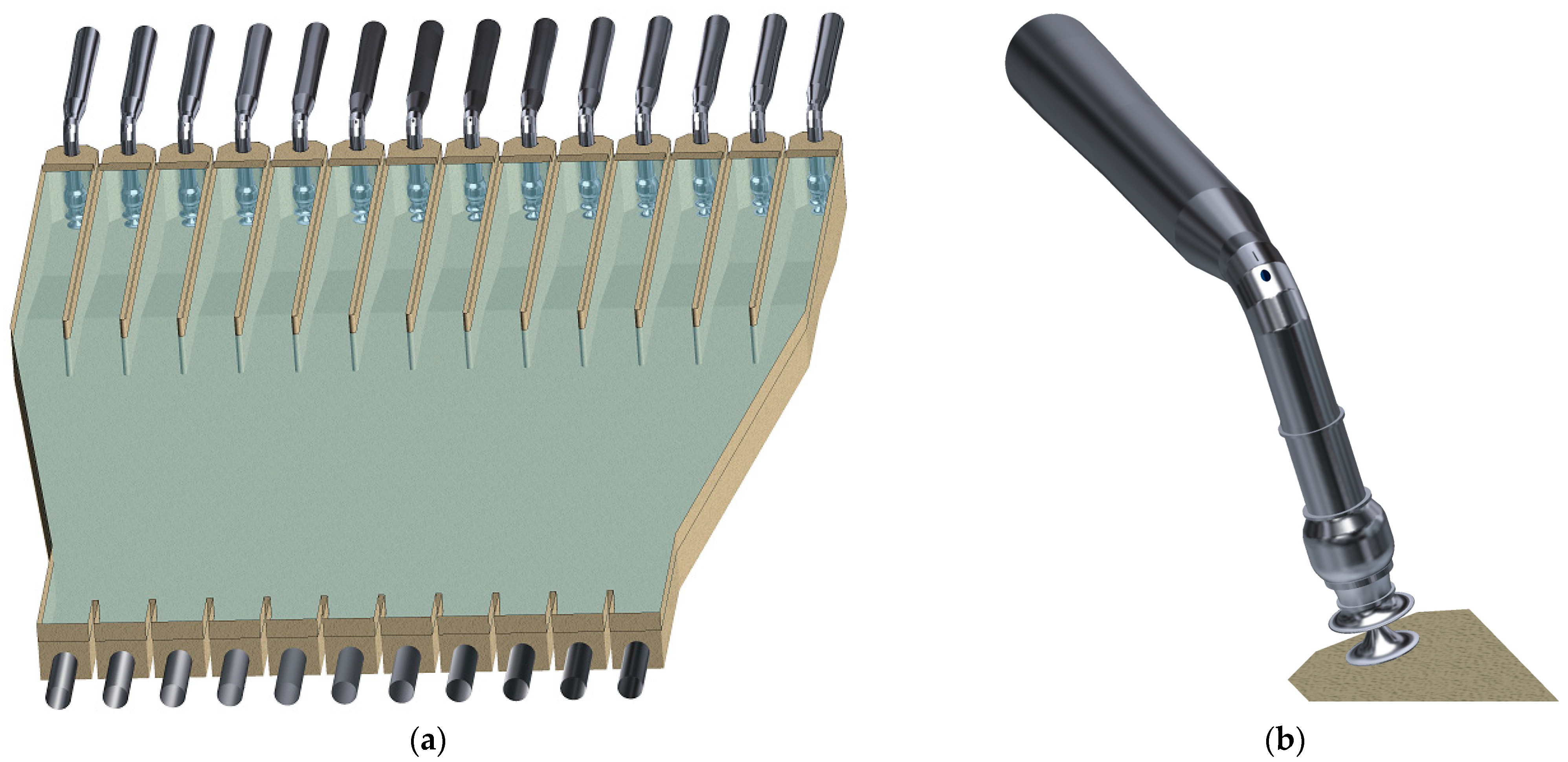
This study deals with a virtual pumping station operating a set of 14 mixed-flow pumps with a nominal flow rate Q = 10.29 m³/s and speed of 400 rpm. These pumps are installed in the suction/intake object, each in its own basin bounded by the concrete pillars (Figure 1a). The width of the basin between the pillars is 5 m and the thickness of the pillars is 0.6 m (Figure 1a). The Low Water Level (LWL) is 6.65 m above the floor at the position of pump. Details of the pump design are shown in Figure 1b and Figure 2a. The pump with a specific speed n_q = 94 has an impeller with five blades and a stator with nine vanes. The pump is equipped with a suction bell and an anti-rotating device, represented by a cone with one vane mounted on the downstream side of the cone. Behind the pump casing, a welded 90° elbow is installed. Each pump is connected with the discharge object by the piping 2970 m long, with a diameter of DN 2500, ending with a welded siphon (Figure 3) equipped with two siphon-breaking valves. The piping has a complicated altitudinal scheme with the maximum difference of the static head of 27.83 m. The shape of the considered terrain is not flat or simply inclined, and the piping must copy the ground. For this reason, the altitudinal scheme in Figure 4 is divided into several intervals with significant slant changes. Three intervals are ascending (corresponding to the pump convention) while the other three are descending. At about 42% of the horizontal distance, the piping reaches nearly the same relative spot height (26 m) as the discharge object.

The volume of water inside one piping is approximately 14,580 m³, which makes the overall volume of water in the discharge piping system about 204,120 m³, which would return to the suction object in the case of an accidental shutdown.

In this study, the following definition of the dimensionless speed n_ED, the dimensionless flow rate Q_ED and the dimensionless torque T_ED is used [46], as described in equation system (1):

n_ED = nD/60/(gH)^0.5   
Q_ED = Q/D²/(gH)^0.5
T_ED = T/D³/(ρgH)   

(1)

where n is the rotor speed [rpm], D is the impeller diameter [m], H is the head [m], Q is the flow rate [m³/s] and T is the torque [Nm].

2.2. Computational Domain and CFD Analysis Settings

Calculations are based on the unsteady Reynolds-Averaged Navier–Stokes equations (URANS):

$$\begin{array}{c}\frac{\partial U_i}{\partial x_i}=0,\\ \frac{\partial \rho U_i}{\partial t}+\frac{\partial {(\rho U}_i{U}_j)}{\partial x_j}=-\frac{\partial P}{\partial x_i}+\frac{\partial }{\partial x_j}\lfloor \left(\mu +{\mu }_t\right)\left(\frac{\partial U_i}{\partial x_j}+\frac{\partial U_j}{\partial x_i}\right)\rfloor +S_{M,i},\end{array}$$

(2)

where U_i are the Reynolds-averaged velocity components in the 3D Cartesian coordinate system, ρ is the fluid density, P is the Reynolds-averaged static pressure, μ is the dynamic viscosity, μ_t is the turbulent viscosity obtained from the turbulence model and S_M is the general momentum source term (here, representing the gravity forces).

The SST turbulence model has been applied. It blends the standard k-ε and k-ω models using two blending functions (F1 and F2) which are dependent on the dimensionless wall distance. The turbulence model can be described by the following governing equations:

$$\begin{array}{c}\frac{\partial \rho k}{\partial t}+\frac{\partial \left({\rho U}_{j}k\right)}{\partial x_j}=\frac{\partial }{\partial x_j}\left[\left(\mu +\frac{{\mu }_t}{{\sigma }_{k3}}\right)\frac{\partial k}{\partial x_j}\right]+P_k-{\beta }^{*}\rho k\omega ,\\ \frac{\partial \rho \omega }{\partial t}+\frac{\partial \left({\rho U}_j\omega \right)}{\partial x_j}=\frac{\partial }{\partial x_j}\left[\left(\mu +\frac{{\mu }_t}{{\sigma }_{\omega 3}}\right)\frac{\partial \omega }{\partial x_j}\right]+{\frac{\gamma \rho }{{\mu }_t}P}_k-{\beta }_3\rho {\omega }^2+\left(1-F1\right)\frac{2\rho }{{\sigma }_{\omega 2}\omega }\frac{\partial k}{\partial x_j}\frac{\partial \omega }{\partial x_j},\end{array}$$

(3)

where

$$P_k={\mu }_t\left(\frac{\partial U_i}{\partial x_j}+\frac{\partial U_j}{\partial x_i}\right)\frac{\partial U_i}{\partial x_j}$$

(4)

is the turbulence production term, k is the turbulent kinetic energy and ω is the turbulent frequency. The turbulent viscosity is described in the following formula:

$${\mu }_t=\frac{\rho a_{1}k}{\mathrm{m}\mathrm{a}\mathrm{x}(a_1\omega ,SF2)}.$$

(5)

where S is the strain rate. During the last two decades, the SST model became a highly valued turbulence model for a wide range of industrial applications. It is very robust and enables us to solve problems with high adverse pressure gradients and separated and swirling flows. More details of the Menter’s SST model, including a definition and discussion of the blending functions and all used constants (a, β, σ, γ), can be found in [47,48].

There are two computational domains for the CFD analysis: the suction object including all pumps (Figure 1 and Figure 2) and the discharge object with all siphons (Figure 3). These two domains are linked with the 1D dynamic model representing the pipeline shown in Figure 4. In reality, the discharge domain is necessary only for the simulations of flow in the pump and reverse pump modes when the pressure losses inside the siphon and in the water jet behind the siphon outlet influence the pump performance curves. With the reversed water flow during the brake/dissipation I mode, the turbine mode, the runaway mode and the break II mode, only the link between the CFD analysis of the suction object and the 1D dynamic model representing the pipeline is considered. There are also the remaining modes of the full 4-quadrant behavior: the brake III mode, the reverse turbine mode and the brake IV mode; these are the artificial modes, which could be reached only inside a special test rig. This is why these modes were simulated in this study in the configuration which corresponds to the closed experimental test rig, as shown in Figure 5. Of course, in this case, the computational domain does not include the complete test rig, and the main tank and fittings are replaced by the straight pipes in front of the pump and behind the elbow so as to set the boundary conditions correctly. Figure 6 shows the computational scheme for the determination of the full 4-quadrant representation. A total of 128 operating points were used to cover all the eight modes and identify the runaway operation regime.

The grids of the computational domains were created using the ANSYS ICEM CFD software (Release 2020 R1) as the multi-block ones and represent about 84 mil. grid nodes for the suction object (including pumps) and about 36 mil. grid nodes for the discharge object (Figure 7). When optimizing the grids, it should be taken into account that very complex flow phenomena appear in the computational domain, changing their character and location based on different performance modes. In fact, it was not possible to carry out a typical grid-dependence study relating simply to the number of grid points for all the performance modes. Because the topology and overall quality of the grid are the most important in these simulations, the parameters like the aspect ratio and skewness as well as the near-wall grid resolution were preferred during the optimization, and the meshes were limited in their size just by the requirement to be able to work within the computer operating memory of 1 TB.

The presented CFD analysis was performed with the ANSYS CFX software (Release 2020 R1) [49]. The high-resolution scheme was used for the momentum equations, while the turbulence numerics was based on the first-order scheme. The time discretization was of the second order and used the backward Euler scheme. The multiphase capability was used to model the flow inside the compound, including the free water level. The numerical solution of the free-surface flow was carried out by means of the VOF method. Pumps were modeled with all hydraulic surfaces (Figure 2a) and with the impeller tip clearance. The SST model was applied with an automatic wall treatment. The Multiple Frame of Reference (MFR) capability in which different domains are rotating relative to one another and the fully-unsteady model of flow (known usually as the Transient Rotor–Stator or the Sliding Mesh) inside the entire pump were used to capture the interactions between the stationary parts inside the pump set and the rotating components. The time steps for the rotation speeds above 300 rpm corresponded to the rotor revolution by 2°; consequently, one rotor revolution represented 180 time steps. For lower rotational speeds, time steps were proportionally decreased to capture the flow dynamics sufficiently. The residuals of the primary variables were set to 10⁻⁴, and the integral values (like head, power input/output, mass flow rate, axial and radial forces) were also evaluated during the time steps in order to monitor the convergence and periodicity of the unsteady solution.

The boundary conditions in the suction object were specified as follows: for the pump and the reverse pump modes, the same velocity and turbulent kinetic energy and its dissipation rate were prescribed at the suction tubes (eleven located at the basin inlet) according to the flow rate and the estimated turbulence intensity and eddy length scale. At the outlets (ends of fourteen pipes behind pumps), the same pressure outlet boundary condition was set for all running pumps. Two transient rotor–stator interfaces were located between the suction object and the impeller and between the impeller and the diffuser of each pump. In the rotating domain, the impeller shroud was treated as the counter-rotating wall. The pump and piping metal walls are supposed to be smooth but all concrete walls of the suction and discharge objects were treated as rough ones, with an equivalent sand roughness of 2 mm. For the brake I, brake II and turbine modes, at each pump discharge piping (behind the elbow), the total pressure, the velocity direction normal to the boundary and the turbulence intensity and its dissipation rate were prescribed. At the suction tubes entry, the same static pressure was set as the outlet condition. For the brake III, brake IV and reverse turbine modes, at the pump discharge piping, the total pressure, the velocity direction normal to the boundary and the turbulence intensity and its dissipation rate were prescribed. At the pump inlet piping entry (Figure 5a), the mass flow rate was set as the outlet condition.

The boundary conditions in the discharge object were specified as follows: at the tubes (fourteen located in front of the siphons), the same velocity and turbulent kinetic energy and its dissipation rate were prescribed according to the flow rate and the estimated turbulence intensity and eddy length scale. At the outlet of the basin, the pressure outlet boundary condition was set with respect to the buoyancy and gravity forces.

2.3. 1D Dynamic Model

The 1D dynamic model, based on MOC, links the suction object with pumps (Figure 1 and Figure 2) and the discharge object (Figure 3). As it was already mentioned, for the pump trip event, the discharge domain is necessary only during the simulations of flow in the pump mode because during the time necessary to empty the discharge piping (the brake I and the turbine modes, or in the vicinity of runaway regime), water from the discharge object does not influence the 1D transient analysis. Still, all the piping with the content of water is considered, including the hydraulic losses caused by the friction on the piping walls. The dynamic model also takes into account the inertia of the pump, the electric motor and the gear box given by their manufacturers. The MOC basic scheme is expressed as follows:

n_i+1 = n_i + (T_i/J) × Δt_i

(6)

where n is the speed, T is the total rotor torque and J is the total moment of inertia. The calculation starts with the steady flow rate corresponding to the pumping station design point. After the accidental shutdown, the following computational scheme is adopted (Figure 8) using the precalculated 4-quadrant characteristics:

There are some important sections of the flow analysis due to time. The first section starts with the pump operating in the pump mode (at the design point) and ends with the shut-off point, in which the pump flow rate reaches zero and the delivery head is the same as the station static delivery head. In this section, the inertia of the water mass and rotating inertia of the pump, the electric engine and the gearbox play the most important role.

The second section represents the break regime. The gravitational forces acting on the water as well as the machine’s mechanical losses decrease the shaft’s rotational speed. At the end of this section, the rotation of the impeller stops to prepare the PAT regime. The inertia of the pump, the electric engine and the gearbox play the most important role at this stage, but still, the inclination of the discharge piping just in front of the discharge object is very important, as well.

The third section represents the turbine regime. The water flowing in the opposite direction generates a torque, which is not efficiently utilized, and the shaft speed is typical for the water turbine. The turbine characteristics of the machine play the most important role at this stage. At the end of this section, the torque of the impeller reaches zero, and the runaway speed is reached.

In the fourth, the longest section, the pump works close to the turbine runaway operating regime. Of course, there are also the mass inertia and mechanical losses, which influence the real operating points, but the time scales are quite large and the changes in the shaft speed are less significant. The mechanical losses inside the pump, the electric engine and the gearbox play the most important role at this stage.

3. Results

3.1. Complete 4-Quadrant Characteristics

The 4-quadrant characteristics are shown in Figure 9 as the functions n_ED(Q_ED) and T_ED(Q_ED), with the signum of the dimensionless variables corresponding to the pump convention, and in Figure 10 as the functions Q_ED(n_ED) and T_ED(n_ED), with the signum of the dimensionless variables corresponding to the turbine convention. The characteristics show S-shape instability, which can be seen in detail in Figure 11. In the region of this instability, pulsations of the pressure and the flow rate cause a dispersion of calculated results and an uncertainty in the approximation curve. Also, in the 1D dynamic model, a special algorithm is applied to find the correct branch of the S-shaped curve.

3.2. Pump Regime

The two most important operating modes are the pump regime and the turbine runaway, which are compared in the following paragraphs. The pump regime is the starting point for the complete simulation of the pump trip. The following data postprocessing was performed for the nominal flow rate Q = 10.29 m³/s and a speed of 400 rpm. The global flow pattern inside the suction and discharge objects can be found in Figure 12 and Figure 13, showing the water level in the vicinity of pumps and siphons. As mentioned above, the CFD analysis was performed for the low water level at the suction compound. At this water level, no air enters the pump suction, and the flow is free of the water-level vortices. Still, there are water waves in the suction object spreading towards the pumps and the back wall of the object, resulting in the water elevation rising up to 0.8 m and in the increased strain of the pump casing. On the other hand, in the vicinity of the siphon outlets, a water level depression of about 0.2 m can be observed, which must be taken into account during the siphon optimal design. It must be mentioned that the water level elevation and depression as well as the spreading of the water waves inside the suction and the discharge objects are caused just by the phenomena inside the water tanks and do not reflect any possible wind effects.

In the vicinity of the pump suction, the water flow has quite a complex character. In such a flow pattern, it is very difficult to identify the separated and secondary flows close to the solid surfaces. The most effective tool here is an application of the surface streamlines and their singular points and lines of attachment and separation. Figure 14 and Figure 15 demonstrate the surface streamlines and the velocity distribution on the solid walls in the vicinity of the pump suction. No global separation can be found on the floor. Moreover, the CFD analysis indicates that the flow close to the anti-rotating cone is very uniform without any undesirable and unsteady bottom vortices. There is an increased velocity on the floor in front of the pump (i.e., left of the pump in Figure 15, according to the pump convention flow direction), but the surface streamlines are pretty symmetrical according to the vertical symmetry plane going through the cone vane. Inside the cone itself (Figure 16a), only very small differences in the velocity magnitude can be found according to the circumferential position. Concerning the flow close to the pump casing, two saddle points on the rear part of the lowest and middle flanges (Figure 14b) indicate the 3D separation formed on the rear part of the pump casing, as it can also be seen in Figure 16a.

Vortical structures in the vicinity of the pump suction are visualized in Figure 16 and Figure 17. Velocity streamlines and the distribution of the velocity swirling strength show typical annular vortices in front of the pump casing flanges, remnants of the vortical vortex formed between the cone apex and the impeller nut and a pair of the side-wall vortices. All these calculated vortices are stable and do not cause any flow instabilities propagating into the impeller’s blade-to-blade channels.

Concerning the flow inside the pump impeller and the vaned diffuser, it is very convenient, without any large global separations. Figure 18 shows the visualized backflow regions inside the impeller and diffuser passages. The only remarkable backflow can be linked with the tip clearance flow at the impeller blade tip clearance. Of course, there is also a backflow region in the position, where the shaft is connected to the stator hub. Figure 19 confirms a very uniform velocity distribution at the impeller entry and a very low level of the secondary flow, which reaches, in its magnitude, about 6% of the meridional velocity. Close to the shroud, the dominant meridional velocity shows the apparent influence of the impeller blade position; the presence of the anti-rotating cone causes a drop of the meridional velocity in the section center by 17.5% according to the mean value of 8 m/s. The influence of the impeller blade position can also be observed in the distribution of the circumferential velocity; because of its very low magnitude, the symmetry of the circumferential velocity at the impeller entry is more influenced by supplementary effects (turbulence, low frequency disturbances).

3.3. Turbine Runaway

The turbine runaway data postprocessing was performed for the turbine flow rate Q = 4.33 m³/s and a speed of −400 rpm. The global flow pattern inside the suction object can be found in Figure 20, showing the water level in the vicinity of the pumps. In contrast to the pump regime, there is a water level depression close to the pump (about 0.4 m), which is relatively static, without forming moving waves. Due to a sufficiently high water level, no air is torn down by the water leaving the pump suction bell, and the flow is free of the water-level vortices. This is in contrast to the situation described in [45], where the runner suffers from a very low water level.

In the vicinity of the pump suction, the water flow has a highly complex behavior. Similarly with the pump regime, the surface streamlines and their singular points and lines of attachment and separation are used to identify the separated and secondary flows. Figure 21 and Figure 22 demonstrate the surface streamlines and the velocity distribution on the solid walls in the vicinity of the pump suction. Several singular points and lines of attachment and separation can be found both on the floor and on the anti-rotating cone, but their pattern is rather unsteady, changing the separation zones in time. Owing to the vane located in the rear part of the anti-rotating cone, the surface streamlines on the cone are symmetrical according to the vertical symmetry plane going through the cone vane. Outside the cone, the flow symmetry is significantly disrupted. It can be also seen that the water leaving the pump bell influences the flow in the suction object in quite a wide area with a clear attachment border line and one or two dominant saddle points on the floor in front of the pump (in Figure 22, one saddle point can be seen). Concerning the 3D separation formed on the rear part of the pump casing, the saddle points move below the lowest and middle flanges, but a noticeable stable node of attachment appears above the middle flange (Figure 21).

Vortical structures in the vertical symmetry plane are visualized in Figure 23 and Figure 24. Velocity streamlines and the distribution of velocity swirling strength show a complex structure of large vortices around the lower part of the pump and the bell. Besides the 3D separation formed on the rear part of the pump casing, there is a pair of dominant counter-rotating vortices in front of the pump (Figure 23), influencing the flow in the pump impeller and blocking the suction bell cross-flow area. The boundary of the largest vortex is associated with the above-mentioned border line on the floor in front of the pump. All the calculated vortices are unsteady and cause significant total pressure losses as well as the increased strain of the pump casing. Compared to the pump nominal flow (Figure 16 and Figure 17), the velocity swirling strength reaches values more than one order higher (Figure 24). A large extent of the vortical frame in the vicinity of the pump suction can be seen (in 3D view) in Figure 25. In front of the pump, a horizontal core of the largest dominant vortex can be seen in Figure 25a. It does not extend to the side walls and turns to two vortex tubes parallel to the side walls. On the other hand, vortices connecting the pump with both the side walls and the back wall can be clearly seen in Figure 25b.

Concerning the flow inside the pump impeller and the vaned diffuser, large global separations can be seen in both components (Figure 26). There is a large separation close to the position, where the shaft connects the stator hub and a remarkable backflow close to the impeller shroud. In Figure 26a, a large backflow region can also be found in the impeller passages close to the hub. It represents an uneven rotating stall [36], which can be better seen in Figure 27, presenting the velocity streamlines inside the impeller in the blade-to-blade transformation. At a 10% span (close to the hub), large separations can be found on the suction as well as the pressure sides of two blades (No. 2, 5). The upper blade-to-blade channel (between blades 1–2) is fully blocked with a large vortex which induces low-frequency pressure pulsations. The speed of the vortex propagation is very low, which is below the impeller’s angular velocity. With increasing blade span, the blocking vortex disappears, as it can be seen in Figure 27 at 90% span (close to the shroud). In Figure 26b, the backflow regions formed on the shroud side close to the trailing edges of the diffuser vanes show some rotational asymmetry; nevertheless, it has a static behavior and can be linked to the influence of the welded 90° elbow upstream of the diffuser.

Figure 28 shows the meridional and circumferential velocity distribution at the impeller entry. These velocities are non-uniform, and, moreover, the circumferential velocities are comparable with the meridional velocities in their maximum module. Close to the center of section AA-AA, a low velocity core appears, which can be linked to the vortices in front of the pump, blocking the pump bell’s cross-flow area (Figure 23).

3.4. PAT during Time Necessary to Empty Discharge Piping

As it has been mentioned already, the calculation starts with the steady flow rate corresponding to the pumping station design point. After the accidental shutdown, the following sections of flow regime appear. The first section starts with the pump operating in the pump mode and ends with the shut-off point, in which the pump flow rate reaches zero and the delivery head is the same as the station’s static delivery head. The second section represents a break regime. At the end of this section, the rotation of the impeller stops to prepare the PAT regime. In the third section, representing the turbine regime, the water flows in the opposite direction, and the shaft speed is typical of the water turbine. At the end of this section, the torque of the impeller reaches the zero value, and the runaway speed is reached. In the last, the longest section, the pump works close to the turbine runaway operating regime.

Figure 29 shows the runaway speed: the remaining volume of water inside one discharge piping of the pumping station and the volume flow rate inside one discharge piping with time. Because the piping behind the suction object is both ascending and descending on its way, the runaway speed changes in a complicated way, with some decelerating and accelerating stages. The maximum runner speed during the turbine regime (which can be very important for the gear box as well as for the motor and its cooling) is 527 rpm. The overall time necessary to empty the discharge piping is about 3170 s, and for most of this time, the mean flow rate of PAT is about 5 m³/s. With a set of 14 mixed-flow pumps, the overall flow rate oscillates around 70 m³/s.

4. Discussion

After a pump is accidentally switched off or electric power is lost due to failure and the (possibly existing) valve fails, a large amount of water returns back to the suction basin with serious water waves and a flooding capacity. In the presented case, a set of 14 mixed-flow pumps is installed in the suction/intake object, and the volume of water inside one piping is approximately 14,580 m³, which makes the overall volume of water in the discharge piping system about 204,120 m³, which would return to the suction object in the case of an accidental shutdown. As it can be seen in Figure 30b, a tsunami with a flow rate of more than 140 m³/s appears some 15 min after the power failure. Also, the achieved shaft speed is very important for the pump, the gear box as well as for the motor and its cooling. There are two time intervals when the speed of PAT exceeds 500 rpm (which is assessed as the limit for the long-term operation). The first one starts about 19 s after the power failure and takes about 48 s. The second one is much longer. Due to a complicated altitudinal scheme of the discharge piping, it starts about 23 min after the power failure and takes about 4.3 min. These time intervals can be very important for the selection of the gear box as well as for the electric motor.

The key issue in the link between the CFD and 1D dynamic models is the interpolation process and a smooth transition between different pump performance modes (or points, in which the performance curve stops to act as a function). Both piecewise representations of the 4-quadrant characteristics (e.g., Q_ED(n_ED) and n_ED(Q_ED), the same for torque) are necessary for an appropriate evaluation; or a piecewise representation Q_ED(s), T_ED(s) and n_ED(s) can be used with an artificial parameter s. Both methods were tested; the second one is slightly faster, nevertheless MOC is much faster than the CFD part of the simulations, and the speed of interpolation plays a minor role. Very important is the algorithm selecting the correct branch of the S-shaped curve because when the pump works close to the turbine runaway operating regime, due to the mass inertia and mechanical losses, the real operating points oscillate between the Turbine and Brake2 modes. In this algorithm, some more factors (e.g., the change in the piping inclination) should be considered.

A very important part of the numerical simulation is the possibility to verify the results with the experimental data. In the presented study, there was an intention to verify the possibility of the CFD simulation to capture the instabilities in the 4-quadrant characteristics. Of course, it is very difficult to realize the complete measurements of all eight modes of the characteristics. This is why the comparison of the experimental and numerical results was performed for the pump regime, which experiences instability in the suboptimal flow rates. The experiment was realized in the hydraulic laboratory of the SIGMA Research and Development Institute with a model pump (impeller diameter of 306 mm). The test rig enabled us to measure model pumps with a power input of up to 400 kW, but at the moment, only the pump regime was supported by the test rig equipment. The magnetic-inductive flowmeter of the accuracy class of 0.2% was applied to measure the volume flow rate. For all measurements of the pressure differences, the pressure transducers were used. They worked in the accuracy class of 0.04%. The temperature of the water was measured with the platinum thermometer in the accuracy class of 0.5%. The evaluation of the power input was based on measurements of the torque and shaft speed by means of the torque transducer in the accuracy class of 0.1. Figure 30 shows the comparison of numerically and experimentally obtained characteristics n_ED(Q_ED) and T_ED(Q_ED) with the signum of the dimensionless variables corresponding to the pump convention. It can be seen that there are differences in the dimensionless speed of less than 1% in the stable part of the curve and up to 3% in the unstable region. The dimensionless torque shows differences of about 3.5% in the stable part of the curve and up to 9% in the unstable region. These differences can be acceptable considering the fact that in the unstable region, the uncertainty of both the experimental and CFD data highly increases, and in the evaluation of the torque in Figure 30b, the mechanical losses are not included.

As expected, the simulations show very convenient flow conditions at the nominal flow rate, which is utilized under the normal pump station operation. At this flow rate and even at the low water level, no air enters the pump suction, and the flow is free of the unsteady water-level and bottom vortices. Also, no global separation can be found on the floor, and the flow close to the anti-rotating cone is very uniform. On the other hand, the flow inside and outside the pump significantly deteriorates during the turbine runaway regime, which is typical for most of the time necessary to empty the discharge piping after an accidental shutdown. The rotating stall and the S-shape instability revealed by the simulations can result in an overstrain and increased vibrations which are very dangerous for PAT as well as the other mechanical components. All these factors should be taken into account when estimating the MTBR (Mean Time Between Replacements) values and the life cycle cost of the station.

This study does not consider the cavitation analysis of the PAT performance. Highly unsteady cavitation phenomena can be another problem, which can influence all the situations of when the pump trip appears. The cavitation performance of PAT is usually well known for the pump and turbine regimes. But to study, in detail, the cavitation performance of PAT in all the 4-quadrant characteristics, this represents a challenge, which can be the target of future simulations and experimental research.

5. Conclusions

This study describes the abnormal situation when a pump trip appears. To be able to analyze the pump performance during an accidental shutdown, the full 4-quadrant characteristics of the pump was applied in the form of dimensionless variables. The application of the 4-quadrant characteristics relies on the validity of the hydraulic affinity laws, and users should be careful of their range. On the other hand, the creation of the dimensionless representation of the 4-quadrant characteristics gives the possibility to repeat calculations for different scenarios and initial states in real time without the necessity of repeated CFD simulations, which are very time-consuming. This is fully in line with the concept of the “digital product passport”, enabling us to solve all critical events in real time based on the necessary data provided by the supplier.

There is one more aspect of the applications of the 4-quadrant characteristics: they are usually derived through experimental configurations with respect to the closed hydraulic test rig. There are also some results obtained for the pumps with the suction elbow/draft tube; however, there are practically no available data related to the pumps with suction bells. This study, therefore, aimed (at least for the most important performance modes) to simulate a real vertical position of the pump in the suction basin with the anti-rotating cone and the free water level.

This paper shows a detailed insight into the two most important operating modes that appear during the pump trip event: pump regime and turbine runaway. The aim is to show completely different flow phenomena inside and in the vicinity of the pump as well as the completely different behaviors of the water level in the suction object. These differences should be taken into account during the design of the pump suction bell, the AVD device as well as the shape of the pump sump. It must be also stressed that the highly unsteady complex phenomena appearing inside and in the vicinity of a pump during some operating modes cannot be modeled in real time in a two-way CFD-1D dynamic model, even with the support of supercomputer facilities. There are also the stability and convergence difficulties, which do not allow us to use a fully automatic generation of CFD data and require full control over the computational processes.

References

1. Kim, C.G.; Kim, B.H.; Bang, B.H.; Lee, Y.H. Experimental and CFD analysis for prediction of vortex and swirl angle in the pump sump station model. IOP Conf. Ser. Mater. Sci. Eng. 2015, 72, 042044. [Google Scholar] [CrossRef]
2. Park, I.; Kim, H.-J.; Seong, H.; Rhee, D.S. Experimental Studies on Surface Vortex Mitigation Using the Floating Anti-Vortex Device in Sump Pumps. Water 2018, 10, 441. [Google Scholar] [CrossRef]
3. Tokyay, T.; Constantinescu, G. Coherent structures in pump-intake flows: A large eddy simulation (LES) study. In Proceedings of the Korea Water Resources Association Conference, Seoul, Republic of Korea, 11–16 September 2005; pp. 231–232. [Google Scholar]
4. Okamura, T.; Kamemoto, K.; Matsui, J. CFD prediction and model experiment on suction vortices in pump sump. In Proceedings of the 9th Asian International Conference on Fluid Machinery, Jeju, Republic of Korea, 16–19 October 2007. [Google Scholar]
5. Bayeul-Lainé, A.C.; Bois, G.; Issa, A. Numerical simulation of flow field in water-pump sump and inlet suction pipe. IOP Conf. Ser. Earth Environ. Sci. 2010, 12, 012083. [Google Scholar] [CrossRef]
6. Long, N.I.; Shin, B.R.; Doh, D.-H. Study on Surface Vortices in Pump Sump. J. Fluid Mach. 2012, 74, 60–66. [Google Scholar] [CrossRef]
7. Amin, A.; Kim, B.H.; Kim, C.G.; Lee, Y.H. Numerical Analysis of Vortices Behavior in a Pump Sump. IOP Conf. Ser. Earth Environ. Sci. 2019, 240, 032020. [Google Scholar] [CrossRef]
8. Shrestha, U.; Choi, Y.D. Bellmouth Shape Optimization for the Suppression of Flow Instability in a Pump Sump Model. KSFM J. Fluid Mach. 2021, 24, 49–57. [Google Scholar] [CrossRef]
9. Zhang, B.; Cheng, L.; Zhu, M.; Jiao, W.; Zhang, D. Numerical Simulation and Analysis of the Flow Characteristics of the Roof-Attached Vortex (RAV) in a Closed Pump Sump. Machines 2022, 10, 209. [Google Scholar] [CrossRef]
10. Kim, S.; Kim, C.; Kim, B.; Jang, H.; Kim, I.; Lee, Y.-H. A Study Comparing the Subsurface Vortex Characteristics in Pump Sumps. Energies 2022, 15, 5049. [Google Scholar] [CrossRef]
11. Uruba, V.; Procházka, P.; Sedlář, M.; Komárek, M.; Duda, D. Experimental and Numerical Study on Vortical Structures and their Dynamics in a Pump Sump. Water 2022, 14, 2039. [Google Scholar] [CrossRef]
12. Chen, Q.; Dai, G.; Liu, H. Volume of Fluid Model for Turbulence Numerical Simulation of Stepped Spillway Overflow. J. Hydraul. Eng. 2002, 128, 7. [Google Scholar] [CrossRef]
13. Larsen, T.; Nielsen, L.; Jensen, B.; Christensen, E.D. Numerical 3-D modelling of Overflows. In Proceedings of the 11th International Conference on Urban Drainage, Edinburgh, Scotland, 31 August–5 September 2008; pp. 1–7. [Google Scholar]
14. Lv, X.; Zou, Q.; Reeve, D. Numerical simulation of overflow at vertical weirs using a hybrid level set/VOF method. Adv. Water Resour. 2011, 34, 1320–1334. [Google Scholar] [CrossRef]
15. Jiang, L.; Diao, M.; Sun, H.; Ren, Y. Numerical Modeling of Flow Over a Rectangular Broad-Crested Weir with a Sloped Upstream Face. Water 2018, 10, 1663. [Google Scholar] [CrossRef]
16. Sedlář, M.; Machalka, J.; Komárek, M. Modeling and Optimization of Multiphase Flow in Pump Station. J. Phys. 2020, 1584, 012070. [Google Scholar] [CrossRef]
17. Zhu, H.; Zhu, G.; Lu, W.; Zhang, Y. Optimal hydraulic design and numerical simulation of pumping systems. Procedia Eng. 2012, 28, 75–80. [Google Scholar] [CrossRef]
18. Liu, Y.; Zhou, J.; Zhou, D. Transient flow analysis in axial-flow pump system during stoppage. Adv. Mech. Eng. 2017, 9, 1687814017723280. [Google Scholar] [CrossRef]
19. Sedlář, M.; Procházka, P.; Komárek, M.; Uruba, V.; Skála, V. Experimental Research and Numerical Analysis of Flow Phenomena in Discharge Object with Siphon. Water 2020, 12, 3330. [Google Scholar] [CrossRef]
20. Furst, J.; Halada, T.; Sedlář, M.; Krátký, T.; Procházka, P.; Komárek, M. Numerical analysis of flow phenomena in discharge object with siphon using lattice-Boltzmann method and CFD. Mathematics 2021, 9, 1734. [Google Scholar] [CrossRef]
21. Hirt, C.W.; Nichols, B.D. Volume of fluid (VOF) method for the dynamics of free boundaries. J. Comput. Phys. 1981, 39, 201–225. [Google Scholar] [CrossRef]
22. Höller, S.; Benigni, H.; Jaberg, H. Numerical and Experimental Investigation of the 4-Quadrant Behavior of Different Mixed Flow Diffuser Pumps. Int. J. Turbomach. Propuls. Power 2019, 4, 3. [Google Scholar] [CrossRef]
23. Höller, S.; Benigni, H.; Jaberg, H. Investigation of the 4-Quadrant behaviour of a mixed flow diffuser pump with CFD-methods and test rig evaluation. IOP Conf. Ser. Earth Envir. Sci. 2016, 49, 032018. [Google Scholar] [CrossRef]
24. Couzinet, A.; Gros, L.; Pierrat, D. Characteristics of Centrifugal Pumps Working in Direct or Reverse Mode: Focus on the Unsteady Radial Thrust. Int. J. Rotating Mach. 2013, 2013, 279049. [Google Scholar] [CrossRef]
25. Bolaños, H.D.; Botero, F. Four quadrant characterization of hydrodynamic phenomena in a low specific speed centrifugal pump. Ing. Univ. 2021, 25, 1–22. [Google Scholar] [CrossRef]
26. Dorfler, P.K. Improved Suter transform for pump-turbine characteristics. Int. J. Fluid Mach. Syst. 2010, 3, 332–341. [Google Scholar] [CrossRef]
27. Biner, D.; Alligné, S.; Hasmatuchi, V.; Nicolet, C.; Hugo, N.; Avellan, F.; Dujic, D.; Münch-Alligné, C.; Dujic, D.; Nicolet, C. Turbine mode start-up simulation of a FSFC variable speed pump-turbine prototype—Part II: 3-D unsteady CFD and FEM. IOP Conf. Ser. Earth Environ. Sci. 2021, 774, 012070. [Google Scholar] [CrossRef]
28. Alligné, S.; Béguin, A.; Biner, D.; Münch-Alligné, C.; Hasmatuchi, V.; Hugo, N.; Avellan, F.; Dujic, D.; Nicolet, C. Turbine mode start-up simulation of a FSFC variable speed pump-turbine prototype—Part I: 1D simulation. IOP Conf. Ser. Earth Environ. Sci. 2021, 774, 012052. [Google Scholar] [CrossRef]
29. Casartelli, E.; Ryan, O.; Schmid, A.; Mangani, L. CFD simulation of transient startup for a low specific-speed pump-turbine. IOP Conf. Ser. Earth Environ. Sci. 2019, 240, 082007. [Google Scholar] [CrossRef]
30. Riedelbauch, S.; Stens, C. Pump to turbine transient for a pump-turbine in a model test circuit and a real size power plant. IOP Conf. Ser. Earth Environ. Sci. 2019, 240, 072039. [Google Scholar] [CrossRef]
31. Stens, C.; Riedelbauch, S. Investigation of a fast transition from pump mode to generating mode in a model scale reversible pump turbine. IOP Conf. Ser. Earth Environ. Sci. 2016, 49, 112001. [Google Scholar] [CrossRef]
32. Liu, W.C.; Zheng, J.S.; Cheng, J.; Shi, Q.H. Hydraulic optimization of “S” characteristics of the pump-turbine for Xianju pumped storage plant. IOP Conf. Ser. Earth Environ. Sci. 2012, 15, 032034. [Google Scholar] [CrossRef]
33. Gentner, C.; Sallaberger, M.; Widmer, C.; Braun, O.; Staubli, T. Numerical and experimental analysis of instability phenomena in pump turbines. IOP Conf. Ser. Earth Environ. Sci. 2012, 15, 032042. [Google Scholar] [CrossRef]
34. Liu, D.; Liu, X. Numerical optimization on the “S” characteristics of model pump-turbine. In Proceedings of the 16th International Symposium on Transport Phenomena and Dynamics of Rotating Machinery, Honolulu, HI, USA, 10–15 April 2016; p. hal-0189441. [Google Scholar]
35. Lenarcic, M.; Gehrer, A. A theoretical, numerical and experimental analysis of S-shape instabilities in reversible pump-turbines: Resultant strategies for improving operational stability. IOP Conf. Ser. Earth Environ. Sci. 2019, 240, 032023. [Google Scholar] [CrossRef]
36. Chen, Z.; Jiang, Z.; Chen, S.; Zhang, W.; Zhu, B. Experimental and numerical study on flow instability of pump-turbine under runaway conditions. Renew. Energy 2023, 210, 335–345. [Google Scholar] [CrossRef]
37. Yang, S.; Li, P.; Tao, R.; Zhang, F.; Xiao, R.; Liu, V.; Wang, F. Investigate the full characteristic of a centrifugal pump-as-turbine (PAT) in turbine and reverse pump modes. Eng. Appl. Comput. Fluid Mech. 2023, 17, 2246527. [Google Scholar] [CrossRef]
38. Zhu, B.; Han, W.; Tai, Z.; Chen, Y. Flow Evolution and Energy Loss Mechanism in Accidental Shutdown Process of a Large Submersible Mixed-Flow Pump System. J. Appl. Fluid Mech. 2023, 16, 947–959. [Google Scholar] [CrossRef]
39. Wang, P.; Luo, X.; Lu, J.; Gao, J.; Cai, Q. Influence of Tubular Turbine Runaway for Back Pressure Power Generation on the Stability of Circulating Cooling Water System. Water 2022, 14, 2294. [Google Scholar] [CrossRef]
40. Sun, Z.; Yu, J.; Tang, F.; Ge, H.; Yuan, H. Analysis of Transient Characteristics of Submersible Tubular Pump During Runaway Transition. Front. Energy Res. 2022, 10, 894796. [Google Scholar] [CrossRef]
41. Kan, K.; Xu, Z.; Chen, Z.; Xu, H.; Zheng, Y.; Zhou, D.; Muhirwa, A.; Maxime, B. Energy loss mechanisms of transition from pump mode to turbine mode of an axial-flow pump under bidirectional conditions. Energy 2022, 257, 124630. [Google Scholar] [CrossRef]
42. Zhou, F.; Li, Q.; Xin, L. Analysis of Vortex Evolution in the Runner Area of Water Pump Turbine under Runaway Conditions. Processes 2023, 11, 2080. [Google Scholar] [CrossRef]
43. Xu, L.; Liu, D.; Li, Z.; Zhao, X.; Liu, X. Experimental and numerical simulation research on flow characteristics of model pump-turbine in four-quadrant operating quadrants. J. Energy Storage 2022, 54, 105083. [Google Scholar] [CrossRef]
44. Li, Z.; Zeng, H.; Wang, K.; Peng, X.; Yan, S.; Qin, Z. Study on S-shaped region of pump turbine based on Omega vortex analysis method and entropy production theory. Int. J. Agric. Biol. Eng. 2023, 16, 102–109. [Google Scholar] [CrossRef]
45. Bahreini, A.; Riasi, A.; Quaranta, F.; Nourbakhsh, A. Numerical and experimental study of a very low head (VLH) turbine in an open channel at no-load conditions. Sustain. Energy Technol. Assess. 2023, 60, 103429. [Google Scholar] [CrossRef]
46. IEC 62097; Hydraulic Machines, Radial and Axial—Methodology for Performance Transposition from Model to Prototype. IEC: Geneva, Switzerland, 2019.
47. Menter, F.R. Two-equation eddy-viscosity turbulence models for engineering applications. AIAA J. 1994, 32, 1598–1605. [Google Scholar] [CrossRef]
48. Raje, P.; Sinha, K. Anisotropic SST turbulence model for shock-boundary layer interaction. Comp. Fluids. 2021, 228, 105072. [Google Scholar] [CrossRef]
49. ANSYS, Inc. ANSYS CFX-Solver Theory Guide; Release 2020 R1; © ANSYS, Inc.: Canonsburg, PA, USA, 2020. [Google Scholar]
Figure 1. Pump station intake: (a) 3D view of complete intake object; (b) detail of mixed-flow pump in one pump sump.
Processes 12 00630 g001
Figure 2. Mixed-flow pump: (a) 3D view of inner components of pump and suction cone; (b) details of pump computational grid.
Processes 12 00630 g002
Figure 3. Pump station discharge: (a) 3D view of complete discharge object; (b) detail of welded siphon.
Processes 12 00630 g003
Figure 4. Simplified altitudinal scheme of discharge piping.
Processes 12 00630 g004
Figure 5. Pump configuration for artificial modes of 4-quadrant characteristics: (a) 3D view of computational model; (b) experimental set-up.
Processes 12 00630 g005
Figure 6. Computational scheme for determination of full 4-quadrant representation. Eight modes and indication of runaway operation.
Processes 12 00630 g006
Figure 7. Pump station computational grid: (a) detail of intake object; (b) detail of discharge object.
Processes 12 00630 g007
Figure 8. Chart of methodology used.
Processes 12 00630 g008
Figure 9. The 4-quadrant characteristics shown as a function of dimensionless flow rate employing the signum of dimensionless variables corresponding to pump convention: (a) nED(QED); (b) TED(QED).
Processes 12 00630 g009
Figure 10. The 4-quadrant characteristics shown as functions of dimensionless speed employing the signum of dimensionless variables corresponding to turbine convention: (a) QED(nED); (b) TED(nED).
Processes 12 00630 g010
Figure 11. Detail of S-shaped characteristics of PAT and uncertainty of calculated data.
Processes 12 00630 g011
Figure 12. Free water level as vertical difference from low water level. Pump nominal flow rate: (a) suction object, vicinity of pumps; (b) discharge object, vicinity of siphons.
Processes 12 00630 g012
Figure 13. Distribution of water volume fraction in pump symmetry plane. Pump nominal flow rate: (a) suction object, vicinity of pump; (b) discharge object, vicinity of siphon.
Processes 12 00630 g013
Figure 14. Suction object, vicinity of pump. Pump nominal flow rate: (a) distribution of velocity; (b) surface streamlines of water.
Processes 12 00630 g014
Figure 15. Velocity streamlines in vicinity of bottom wall and anti-rotating cone. Pump nominal flow rate.
Processes 12 00630 g015
Figure 16. Suction object, vicinity of pump. Pump nominal flow rate: (a) velocity streamlines in pump symmetry plane; (b) velocity swirling strength.
Processes 12 00630 g016
Figure 17. A 3D visualization of vortical structures in vicinity of bottom wall and anti-rotating cone; pump nominal flow rate. Isosurface of velocity swirling strength, 2 s−1.
Processes 12 00630 g017
Figure 18. The 3D view of backflow regions inside impeller and diffuser. Pump nominal flow rate: (a) front view; (b) rear view.
Processes 12 00630 g018
Figure 19. Suction object, section AA-AA. Pump nominal flow rate: (a) meridional velocity; (b) circumferential velocity.
Processes 12 00630 g019
Figure 20. Suction object, vicinity of pumps. Turbine runaway: (a) free water level as vertical difference from low water level; (b) distribution of water volume fraction in pump symmetry plane.
Processes 12 00630 g020
Figure 21. Suction object, vicinity of pump. Turbine runaway: (a) distribution of velocity; (b) surface streamlines of water.
Processes 12 00630 g021
Figure 22. Velocity streamlines in vicinity of bottom wall and anti-rotating cone. Turbine runaway.
Processes 12 00630 g022
Figure 23. Suction object, vicinity of pump, turbine runaway: (a) velocity streamlines in pump symmetry plane; (b) velocity vectors in pump symmetry plane.
Processes 12 00630 g023
Figure 24. Suction object, vicinity of pumps, turbine runaway. Velocity swirling strength in pump symmetry plane: (a) scale corresponding to Figure 16b; (b) extended quantity scale.
Processes 12 00630 g024
Figure 25. The 3D visualization of vortical structures in vicinity of bottom wall and anti-rotating cone. Turbine runaway. Isosurface of velocity swirling strength, 7 s−1: (a) front view; (b) rear view.
Processes 12 00630 g025
Figure 26. The 3D view of backflow regions inside impeller and diffuser. Turbine runaway: (a) front view; (b) rear view.
Processes 12 00630 g026
Figure 27. Velocity inside impeller in blade-to-blade transformation. From the left: span 0.1, 0.5 and 0.9. Turbine runaway.
Processes 12 00630 g027
Figure 28. Suction object, section AA-AA. Turbine runaway: (a) meridional velocity; (b) circumferential velocity.
Processes 12 00630 g028
Figure 29. Speed, remaining volume of water and volume flow rate inside one piping with time. Positive sign of speed is valid for turbine regime: (a) overall course; (b) details of critical time intervals. Red line represents the critical value level.
Processes 12 00630 g029
Figure 30. Pump regime. Comparison of CFD simulation and experimental data: (a) nED(QED); (b) TED(QED).
Processes 12 00630 g030
Disclaimer/Publisher’s Note: The statements, opinions and data contained in all publications are solely those of the individual author(s) and contributor(s) and not of MDPI and/or the editor(s). MDPI and/or the editor(s) disclaim responsibility for any injury to people or property resulting from any ideas, methods, instructions or products referred to in the content.