Multi-Energy Flow Integrated Energy System Considering Economic Efficiency Targets: Capacity Allocation and Scheduling Study

Abstract

An integrated energy system (IES) breaks down barriers between different energy subsystems, enhancing energy reliability and efficiency. However, issues such as uneven equipment capacity allocation and suboptimal scheduling persist in multi-energy flow IES. To maximize economic benefits while ensuring energy balance and the operational characteristics of the equipment, a capacity matching optimization and scheduling strategy model for IES was developed. Firstly, mathematical models for the electricity, gas, and thermal networks within the IES were established. Secondly, considering the efficiency of energy conversion between different forms and constraints of energy storage in the electricity–thermal–gas interconnected energy system, optimization solutions were obtained using regional contraction algorithms and sequential quadratic programming methods. Finally, case studies conducted in a real park demonstrated that, through optimized capacity matching, unit prices for electricity, heat, and gas decreased by 39.9%, 90.5%, and 74.2%, respectively, effectively improving the economic viability of the system.

1. Introduction

The global economy has been developing rapidly since the beginning of the 21st century, and the world’s demand for energy has been rising year by year. The traditional energy supply system has problems such as a heavy reliance on fossil energy and its low efficiency of energy utilization [1]. In this context, the energy Internet [2], with its low-carbon environmental protection and clean and efficient features, provides a new idea for the study of the future energy system, and integrated energy systems realize the gradient utilization of electricity, heat, gas, and other energy sources, maximizing renewable energy consumption and energy utilization [3].

An integrated energy system converts various forms of energy, such as solar energy, wind energy, biomass energy, etc., into other forms of energy that are required by the consumer body, such as electricity, gas, heat (cold), etc. [4,5]. In recent years, modeling and analysis, optimal scheduling, and performance evaluation for integrated energy systems have become hot topics among researchers worldwide [6,7,8]. Madi et al. [9] conceived an integrated energy system framework with electricity as the core, proposed a coordinated and optimized operation mode and energy conversion method, and explored the key problems in multi-energy operations. Zhang Wendong et al. [10] designed an integrated energy system based on household cooling and heating loads and utilized mixed-integer linear programming methods to optimize the system’s design, determine its main types of equipment, and establish the installed capacity of the system. Wang Yongli et al. [11] established different electric heating and cooling energy systems based on the main equipment of the distributed energy system and established an optimized model of the energy systems to obtain the optimal configuration, operation strategy, and evaluation index values of the different systems. Wang Jun et al. [12] established a multi-energy system unit containing cold energy, heat energy, and electricity and solved the capacity configuration problem of the system. In summary, most of the existing studies on integrated energy systems are limited to pure electric power systems or electric–heat–cooling combined-supply systems, and there are few studies on integrated energy systems coupling electric, thermal, and gas multi-energy flows. However, with the commercialization of fuel cells, the introduction of fuel cell vehicles, and the continuous development of power-to-gas (P2G) technology [13], the demand for hydrogen is becoming more and more widespread, and the future IESs and the establishment of the energy Internet will inevitably include hydrogen energy flows, so optimizing the design of integrated energy systems containing electricity, heat, and gas multi-energy flows has far-reaching significance.

Reversible Solid Oxide Cells (RSOCs) [14] are some of the most advanced types of fuel cells, as they can operate as both a Solid Oxide Fuel Cell (SOFC) for power generation or cogeneration and as a Solid Oxide Electrolytic Cell (SOEC) for hydrogen and oxygen generation through water electrolysis using electric energy. The advantages they offer include their high energy density, long lifespans, high efficiency, absence of self-discharge phenomena during operation, and the fact that their use does not involve depth of discharge or battery capacity limitations. Models related to RSOCs are mostly based on separate physical systems of SOFCs or SOECs and their corresponding control system models. For instance, Pianko-Oprych et al. [15] hierarchically modeled SOFC stacks and analyzed system responses to load changes. Lu Yi et al. [16] analyzed combined hydrogen production systems making use of SOECs, studying the effects of temperature and steam flow rate variations on hydrogen production efficiency. Rispoli et al. [17] applied RSOCs in microgrids, optimizing the capacities of various pieces of equipment within the system with the aim of minimizing the microgrid investment payback period, resulting in a payback period of 6–10 years. RSOCs integrate multiple energy flows of electricity, heat, and gas, enabling the flexible conversion of these energy forms, making them one of the key components for constructing comprehensive energy systems. However, most contemporary comprehensive energy systems are based on either individual fuel cells [18] or a combination of fuel cells and electrolyzers [19], with there being very few studies focusing on optimizing the design of comprehensive energy systems based on RSOCs. This has led to an overly optimistic capacity allocation scheme, which has made it difficult to achieve the expected economic benefits in actual operation.

Table 1. Summary of the literature review.

Reference	System	Objective Function	Electricity	Heat	Hydrogen	RSOC	SOFC	SOEC
[9]	IES	Energy procurement costs and operating costs	√	×	√	×	×	×
[11]	IES	Carbon emissions and operating costs	√	√	×	×	×	×
[15]	SOFC	Operating cost	√	√	√	×	√	×
[16]	SOEC	Maintenance and operating costs	×	√	√	×	×	√
[17]	Microgrid	Investment costs, operation and maintenance costs	√	√	√	×	√	√
Article	IES	Equipment depreciation costs, fuel costs, pollutant costs and O&M costs	√	√	√	√	√	√

compares the advantages of this study’s approach with those of published papers related to multi-energy systems. As can be seen, most of the existing studies are based on using SOFCs or SOECs for design optimization, with studies rarely considering the use of electric, thermal, and gas energy in the system simultaneously. In an attempt to address the above problems, this paper proposes a multi-energy flow IES containing RSOCs; considers the demands of multiple energy forms, including electricity, heat, and gas; and presents a model of the system’s capacity matching optimization and scheduling strategy, with the objective being to maximize its economic efficiency. The system is based on a region contraction algorithm (RCA) [20] and sequential quadratic programming (SQP) optimization solving. The main contributions of this paper are summarized below:

(1)

Most IESs have wind turbines and photovoltaic technology as the primary pieces of power supply equipment. In the system proposed in this paper, an RSOC is used as the auxiliary power supply component, so that the system can be operated in SOFC mode or SOEC mode, and the system also includes energy storage equipment such as batteries, heaters, and hydrogen tanks which do not waste any energy.

(2)

A capacity matching optimization and scheduling strategy model for the proposed multi-energy flow integrated energy system is established. In order to improve the economics of the system, we aimed to realize the system’s lowest energy cost using both the RCA and SQP.

(3)

The proposed RCA and SQP algorithms are compared with different algorithms. Our simulation results verify the effectiveness and economy of the proposed algorithms.

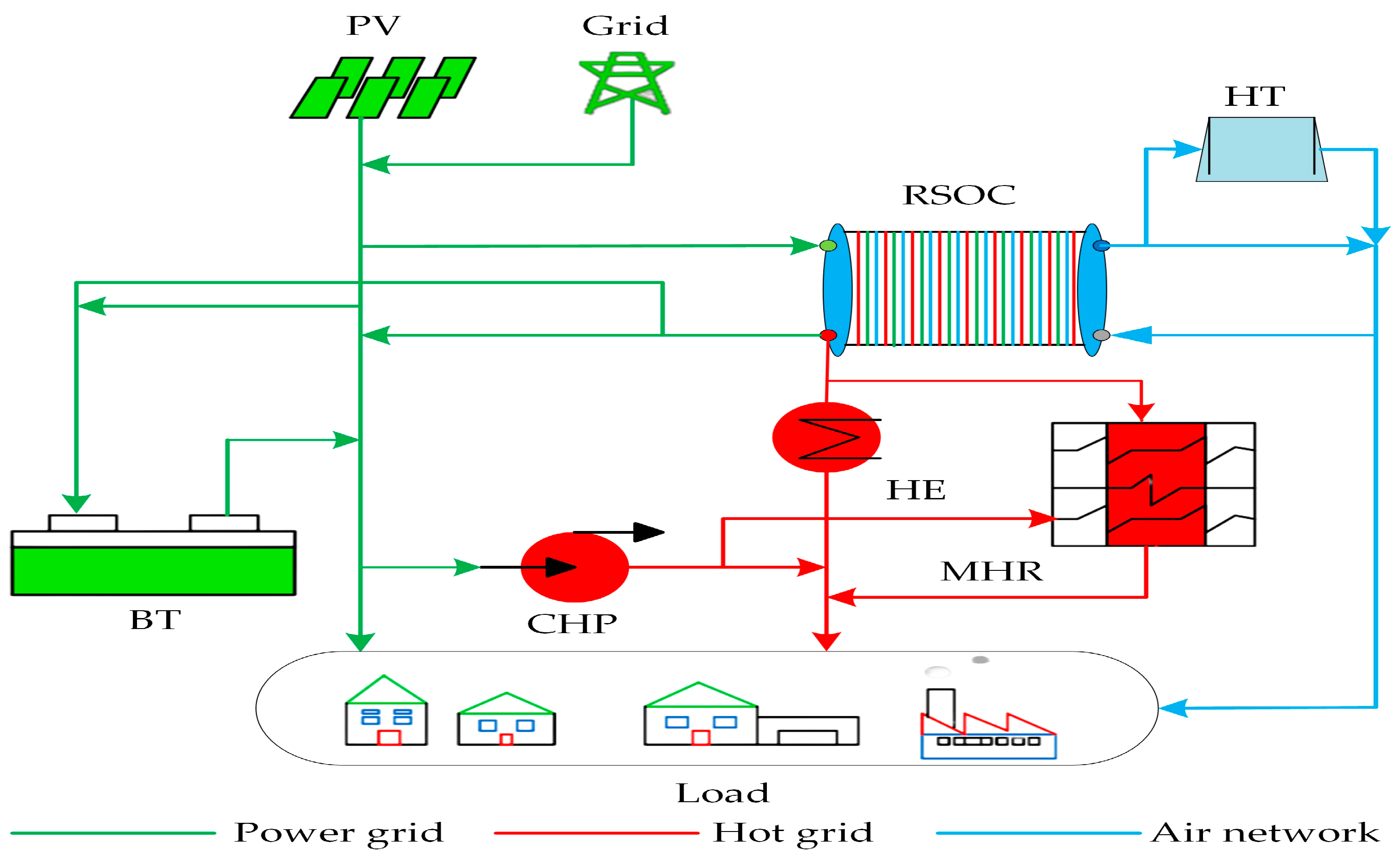
2. Integrated Energy System with Electricity, Heat, and Gas

2.1. System Structure

As shown in Figure 1, the system is divided into three subsystems based on electricity, heat, and gas energy, respectively. Among them, the IES components are divided into three categories: energy conversion components (RSOC, compression heat pumps (CHP), and heat exchangers (HEs)); energy storage components (batteries (BTs), multi-stage storage heaters (MHRs), and hydrogen tanks (HTs)); and distributed renewable energy components (photovoltaic (PV) technology). Electricity, heat, and gas energy flows are coupled with each other and provide energy to the outside world using clean energy as a carrier, as well as energy conversion and storage.

2.2. System Mode of Operation

The choice of operation mode plays a decisive role in the operational performance of integrated energy systems. Currently, there are two typical operation modes: “following the electric loads (FEL)” and “following the thermal loads (FTL)” [21]. Conventional combined-supply systems use the “following the electric loads” mode, which generates excess heat, while the “following the thermal loads” mode generates excess electricity. The system is equipped with energy storage devices such as batteries, heaters, and hydrogen tanks, which can store the excess energy without wasting any energy. In order to meet the demand of each load, the “heat following” operation mode was selected, and the specific operation modes are as follows:

(1)

The RSOC operates in SOFC mode. The excess heat energy generated and CHP work together to meet the heat load of the users, and the excess heat is stored in the MHR. When there is insufficient heat at the peak of heat consumption, the heat in the MHR is prioritized and used, and if the demand is not met, the CHP is used as an auxiliary heat source to provide heat.

(2)

The RSOC operates in SOEC mode. The hydrogen generated is used for the user gas load and the equipment in the system, and the excess hydrogen is stored in a hydrogen storage tank for use when the hydrogen generated by the RSOC is insufficient.

(3)

The PV technology is used as the primary power supply device, and the RSOC is used as the auxiliary power supply device to supply power to the consumer electrical loads and the equipment in the system. Excess power is stored in the storage battery. When the power generated by the system is insufficient, the use of the power in the storage battery is prioritized, and if the demand is not met, connecting to the grid can provide power.

3. Multi-Energy Flow Coupling Calculation Method for the Integrated Energy System

Each element can be equated to a double-ended element for energy input and energy output, differing only in the type of input and output energy, and the multiple energy flows of the IES can be coupled and calculated by linearization. The overall energy inflow and outflow of the IES can be calculated using the following equation:

$$\left[\begin{array}{c}{P}_{\mathrm{e}}^{\mathrm{in}}(t)\\ P_{\mathrm{g}}^{\mathrm{in}}(t)\\ P_{\mathrm{h}}^{\mathrm{in}}(t)\end{array}\right]={\displaystyle \sum _{k\in S_e}{N}_k}\left[\begin{array}{c}{P}_{\mathrm{e},k}^{\mathrm{in}}(t)\\ P_{\mathrm{g},k}^{\mathrm{in}}(t)\\ P_{\mathrm{h},k}^{\mathrm{in}}(t)\end{array}\right]$$

(1)

$$\left[\begin{array}{c}{P}_{\mathrm{e}}^{\mathrm{out}}(t)\\ P_{\mathrm{g}}^{\mathrm{out}}(t)\\ P_{\mathrm{h}}^{\mathrm{out}}(t)\end{array}\right]={\displaystyle \sum _{k\in S_{\mathrm{e}}}{N}_k}\left[\begin{array}{c}{P}_{\mathrm{e},\mathrm{k}}^{\mathrm{out}}(t)\\ P_{\mathrm{g},\mathrm{k}}^{\mathrm{out}}(t)\\ P_{\mathrm{h},\mathrm{k}}^{\mathrm{out}}(t)\end{array}\right]$$

(2)

where: $P_{\mathrm{e}}^{\mathrm{in}}(t),P_{\mathrm{g}}^{\mathrm{in}}(t),P_{\mathrm{h}}^{\mathrm{in}}(t)$ is the electric, gas and heat input of IES at time t; $S_e$ is the set of various types of equipment in IES; $N_k$ is the number of various types of equipment, which can be a continuous or discrete variable depending on the type of equipment; $P_{\mathrm{e},k}^{\mathrm{in}}(t),P_{\mathrm{g},k}^{\mathrm{in}}(t),P_{\mathrm{h},k}^{\mathrm{in}}(t)$ is the electric, gas, and heat input of the kth equipment at time t; $P_{\mathrm{e}}^{\mathrm{out}}(t),P_{\mathrm{g}}^{\mathrm{out}}(t),P_{\mathrm{h}}^{\mathrm{out}}(t)$ is the electric, gas, and heat output of IES at time t; and $P_{\mathrm{e},k}^{\mathrm{out}}(t),P_{\mathrm{g},k}^{\mathrm{out}}(t),P_{\mathrm{h},k}^{\mathrm{out}}(t)$ is the electric, gas, and heat output of the kth device at time t.

Multi-energy devices can be sorted into three categories according to their input and output characteristics: energy conversion components, energy storage components, and distributed renewable energy components.

(1) Energy conversion element input–output model. The input–output power relationship of the energy conversion element is as follows:

$$\left[\begin{array}{c}{P}_{e,k}^{\mathrm{out}}(t)\\ P_{g,k}^{\mathrm{out}}(t)\\ P_{h,k}^{\mathrm{out}}(t)\end{array}\right]=\left[\begin{array}{ccc}{\eta }_{e,k}& {\eta }_{eg,k}& {\eta }_{eh,k}\\ {\eta }_{g,k}& {\eta }_{g,k}& {\eta }_{gh,k}\\ {\eta }_{he,k}& {\eta }_{hg,k}& {\eta }_{hh,k}\end{array}\right]\left[\begin{array}{c}{P}_{e,k}^{\mathrm{in}}(t)\\ P_{g,k}^{\mathrm{in}}(t)\\ P_{h,k}^{\mathrm{in}}(t)\end{array}\right]$$

(3)

where: ${\eta }_{ij,k}$ is the efficiency of the energy conversion element k to convert from energy i to energy j.

Generally, the energy conversion element only converts one form of energy to another, such as CHP converting electrical energy to thermal energy; ${\eta }_{ij,k}$ is the coefficient of performance, so the majority of the elements of the efficiency matrix is zero.

(2) Energy storage element input–output model. The energy storage element is a single-input and single-output element, and the input and output power relationship of energy storage element k for energy i is as follows:

$$S_{i,k}(t)=S_{i,k}(t-1)+[{\eta }_{i,k}^{\mathrm{in}}\times P_{i,k}^{\mathrm{in}}(t)-P_{i,k}^{\mathrm{out}}(t)/{\eta }_{i,k}^{\mathrm{out}}]\mathsf{\Delta }t/E_k$$

(4)

where: $S_{i,k}(t)$ is the percentage of remaining capacity of storage element k at time t, which is the State-of-Charge (SOC) value for the battery; ${\eta }_{i,k}^{\mathrm{in}},{\eta }_{i,k}^{\mathrm{out}}$ is the charging power and discharging efficiency of storage element k; $\mathsf{\Delta }t$ is the scheduling interval; and $E_k$ is the rated capacity of the storage element.

(3) Distributed renewable energy element input–output model. The input of the distributed renewable energy element is renewable energy such as light, which can be regarded as a zero-input single-output element. The upper limit of distributed renewable energy element’s output power is affected by natural conditions. The power output constraints of the distributed renewable energy element are as follows:

$$P_{i,k,\min }^{\mathrm{out}}(t)⩽P_{i,k}^{\mathrm{out}}(t)⩽P_{i,k,\max }^{\mathrm{out}}(t)$$

(5)

where: $P_{i,k}^{\mathrm{out}}(t)$ is the maximum and minimum output power of the distributed renewable energy element k at energy i at time t.

4. System Optimization Model

4.1. Objective Function

In order to determine the optimal capacity matching of each device in the system and the scheduling strategy per unit of time during the simulation cycle so that the system can be optimally economical in providing a stable and reliable energy supply, the energy cost (${\mathcal{C}}^{COE}$) is selected as the optimization objective, i.e., all the costs spent per unit of energy in converting it from other forms of energy to the required energy, including the sum of all the costs, such as the depreciation cost of the equipment (${\mathcal{C}}^{\mathrm{dep}}$), fuel cost ($C^{fue}$), pollutant emission cost ($C^{dam}$), the depreciation cost of the auxiliary equipment ($C_{BOP}^{dep}$), and the operation and maintenance costs of the equipment ($C_{\mathrm{SYS}}^{\mathrm{mai}}$) [22].

Since the internal energy consumption of the system needs to be considered, a multi-level objective equation is used to optimize the thermal, gas, and electronic subsystems. The mth level optimization objective function is denoted by $C_m^{\mathrm{COE}}$ and the optimization level m + 1 > m. The calculation formula is as follows:

$$C_1^{\mathrm{COE}}=\frac{{\displaystyle \sum _{k=1}^M{\displaystyle \sum _{i=1}^T(C_{i,k}^{\mathrm{dep}}+C_{i,k}^{\mathrm{fue}}+C_{i,k}^{\mathrm{dam}})}}+C_{\mathrm{BOP}-\mathrm{T}}^{\mathrm{dep}}+C_{\mathrm{SYS}}^{\mathrm{mai}}}{{\displaystyle \sum _{k=1}^M{d}_k^{\mathrm{Q}}}}$$

(6)

$$C_2^{\mathrm{COE}}=\frac{{\displaystyle \sum _{k=1}^M{\displaystyle \sum _{i=1}^H(C_{i,k}^{\mathrm{dep}}+C_{i,k}^{\mathrm{fue}}+C_{i,k}^{\mathrm{dam}})}}+C_{\mathrm{BOP}-\mathrm{H}}^{\mathrm{dep}}+C_{\mathrm{SYS}}^{\mathrm{mai}}}{{\displaystyle \sum _{k=1}^M{d}_k^{\mathrm{G}}}}$$

(7)

$$C_3^{\mathrm{COE}}=\frac{{\displaystyle \sum _{k=1}^M{\displaystyle \sum _{i=1}^E(C_{i,k}^{\mathrm{dep}}+C_{i,k}^{\mathrm{fue}}+C_{i,k}^{\mathrm{dam}})}}+C_{\mathrm{BOP}-\mathrm{E}}^{\mathrm{dep}}+C_{\mathrm{SYS}}^{\mathrm{mai}}}{{\displaystyle \sum _{k=1}^M{d}_k^{\mathrm{P}}}}$$

(8)

where: M is the number of unit time intervals; T is the number of heating equipment; $d_k^Q$ is the total heat load of the system at k moments, kW; H is the number of gas supply equipment; $d_k^{\mathrm{G}}$ is the total hydrogen load of the system at k moments, m³/h; E is the number of power supply equipment; $d_k^P$ is the total electric load of the system at k moments, kW; $C_{\mathrm{BOP}-\mathrm{T}}^{\mathrm{dep}},C_{\mathrm{BOP}-\mathrm{H}}^{\mathrm{dep}}$ and $C_{\mathrm{BOP}-\mathrm{E}}^{\mathrm{dep}}$ are the depreciation cost of auxiliary equipment for the heat, gas and electronic systems, respectively.

Of these, each cost is specifically represented below:

$$C^{\mathrm{dep}}=\max (C_{\mathrm{phy}}^{\mathrm{dep}},C_{\mathrm{run}}^{\mathrm{dep}})$$

(9)

$$C_{\mathrm{phy}}^{\mathrm{dep}}=\mathsf{\Delta }t\frac{\omega c^{\mathrm{cap}}}{t_{\mathrm{phy}}}$$

(10)

$$C_{\mathrm{run}}^{\mathrm{dep}}=a\frac{\omega c^{\mathrm{cap}}}{p_{\mathrm{life}}}$$

(11)

$$C^{\mathrm{fue}}=a\frac{c^{\mathrm{fue}}}{q_{\nu }\eta }$$

(12)

$$C^{\mathrm{dam}}=p{C}_{\mathrm{coal}}{f}_{\mathrm{coal}}{c}_{{\mathrm{CO}}_2}^{\mathrm{dam}}$$

(13)

where: $C_{\mathrm{phy}}^{\mathrm{dep}}$ is the depreciation cost of individual equipment based on the physical service life of the equipment within a unit time interval; $C_{\mathrm{run}}^{\mathrm{dep}}$ is the depreciation cost of the equipment after considering the impact of the operating status of the equipment on the service life of the equipment; $\mathsf{\Delta }t$ is the time interval, h; $\omega$ is the capacity of the equipment; $c^{\mathrm{cap}}$ is the cost of the equipment per unit of capacity; $t_{phy}$ is the life cycle of the equipment, h; a is the amount of energy supplied by the equipment per unit of time, i.e., the amount of electricity generated, the amount of heat produced, or the amount of gas supplied; $p_{\mathrm{life}}$ is the energy generated over the life cycle of the equipment; $c^{\mathrm{fue}}$ is the unit price of fuel for the equipment; $q_{\nu }$ is the calorific value of the fuel, kW·h/m³; $\eta$ is the operating efficiency of the equipment; p is the amount of electricity supplied by the grid per unit of time interval $\mathsf{\Delta }t$, kW·h; $C_{\mathrm{coal}}$ is the amount of coal consumed by the grid to supply electricity, kg/(kW·h); $f_{\mathrm{coal}}$ is the emission factor; and $C_{{\mathrm{CO}}_2}^{\mathrm{dam}}$ is the tax on carbon emissions.

Since the concept of carbon emission cost is relatively mature at present, the adopted model only considers the emission cost due to CO₂, and IES only has CO₂ emission from the grid, then the pollutant emission cost $C^{\mathrm{dam}}$ can be expressed as Equation (13). The auxiliary system of IES mainly includes components such as AC/DC inverters, cables, pipes, intelligent controllers, etc. The input cost of this part is mainly determined by the load condition, and the depreciation cost of this type of equipment is not directly related to its operating status. The depreciation cost $C_{\mathrm{BOP}}^{\mathrm{dep}}$ of this type of equipment is not directly related to its operating status, so it can be directly calculated according to Equation (10). In this paper, to simplify the calculation, the input cost of the auxiliary system is calculated as 30% of the total initial input cost of the system [23]. The equipment operation and maintenance cost $C_{SYS}^{\mathrm{mai}}$ mainly refers to the labor cost generated by the maintenance and overhaul of the equipment, which is mainly determined by the salary level of the system location. The depreciation cost of RSOC’s equipment is directly related to its operating status, so RSOC’s depreciation cost is calculated according to Equation (11).

4.2. Constraints

4.2.1. Energy Balance Constraints

Energy balance requires that the energy provided by the system meets its own needs while being able to meet the external load’s demand for three types of energy: electricity, heat, and gas, which can be expressed as follows:

$$\sum _{i=1}^E{p}_{i,k}=d_k^{\mathrm{P}}$$

(14)

$$\sum _{i=1}^T{q}_{i,k}=d_k^Q$$

(15)

$$\sum _{i=1}^H{g}_{i,k}=d_k^{\mathrm{G}}$$

(16)

where: $p_{i,k}$ is the power supply of power supply equipment i at k time, kW; $q_{i,k}$ is the heat supply of heating equipment i at k time, kW; $g_{i,k}$ is the gas supply of gas supply equipment i at k time, m³/h.

4.2.2. Equipment Operating Characteristic Constraints

The operating characteristics of each piece of equipment are determined by the energy production process and energy conversion process of the equipment, which can be expressed as follows:

$$p_{\mathrm{PV}}={\eta }_{\mathrm{PV}}{R}_{\mathrm{k}}{\omega }_{\mathrm{PV}}\mathsf{\Delta }t$$

(17)

$$0\le p_{\mathrm{SOFC}}\le {\omega }_{\mathrm{SOFC}}\mathsf{\Delta }t$$

(18)

$$0\le g_{\mathrm{SOEC}}\le {\omega }_{\mathrm{SOEC}}\mathsf{\Delta }t$$

(19)

$$0\le p_{\mathrm{GRID}}\le {\omega }_{\mathrm{GRID}}\mathsf{\Delta }t$$

(20)

$$0\le q_{\mathrm{C}\mathrm{H}\mathrm{P}}\le {\omega }_{\mathrm{C}\mathrm{H}\mathrm{P}}\mathsf{\Delta }t$$

(21)

$$\left\{\begin{array}{c}0\le p_{\mathrm{BT}}\le \min (V_{\mathrm{BT}}^{\mathrm{discharge}}{I}_{\mathrm{MAX}}^{\mathrm{discharge}}\mathsf{\Delta }t,{\omega }_{\mathrm{BT}}{\eta }_{\mathrm{BT}}^{\mathrm{discharge}})\\ \max (-V_{\mathrm{BT}}^{\mathrm{charge}}{I}_{\mathrm{MAX}}^{\mathrm{charge}}\mathsf{\Delta }t,-\frac{{\omega }_{\mathrm{BT}}}{{\eta }_{\mathrm{BT}}^{\mathrm{charge}}})\le p_{\mathrm{BT}}\le 0\end{array}\right.$$

(22)

$$\left\{\begin{array}{c}0.4\le S_k^{\mathrm{C}}=S_{k-1}^{\mathrm{C}}+\frac{p_{\mathrm{BT}}^k}{{\eta }_{\mathrm{BT}}^{\mathrm{discharge}}{\omega }_{\mathrm{BT}}}\le 1\\ 0.4\le S_k^{\mathrm{C}}=S_{k-1}^{\mathrm{C}}+\frac{{\eta }_{\mathrm{BT}}^{\mathrm{charge}}{p}_{\mathrm{BT}}^k}{{\omega }_{\mathrm{BT}}}\le 1\end{array}\right.$$

(23)

$$\left\{\begin{array}{c}0\le q_{\mathrm{MHR}}\le {\omega }_{\mathrm{MHR}}\mathsf{\Delta }t{\eta }_{\mathrm{MHR}}^{\mathrm{rel}}\\ -\frac{{\omega }_{\mathrm{HE}}\mathsf{\Delta }t}{{\eta }_{\mathrm{MHR}}^{\mathrm{rec}}}\le q_{\mathrm{MHR}}\le 0\end{array}\right.$$

(24)

$$\left\{\begin{array}{c}0\le S_k^{\mathrm{H}}=S_{k-1}^{\mathrm{H}}+\frac{q_{\mathrm{MHHR}}^k}{{\eta }_{\mathrm{MHR}}^{\mathrm{rel}}{\omega }_{\mathrm{MHR}}}\le 1\\ 0\le S_k^{\mathrm{H}}=S_{k-1}^{\mathrm{H}}+\frac{{\eta }_{\mathrm{MHR}}^{\mathrm{rec}}{q}_{\mathrm{MHR}}^k}{{\omega }_{\mathrm{MHR}}}\le 1\end{array}\right.$$

(25)

$$\left\{\begin{array}{c}0\le g_{\mathrm{HT}}\le \frac{{\omega }_{\mathrm{HT}}}{{\rho }_{{\mathrm{H}}_2}}\mathsf{\Delta }t{\eta }_{\mathrm{HT}}^{\mathrm{rel}}\\ -\frac{{\omega }_{\mathrm{HT}}\mathsf{\Delta }t}{{\rho }_{{\mathrm{H}}_2}{\eta }_{\mathrm{HT}}^{\mathrm{sto}}}\le g_{\mathrm{HT}}\le 0\end{array}\right.$$

(26)

$$\left\{\begin{array}{c}0\le S_k^{\mathrm{G}}=S_{k-1}^{\mathrm{G}}+\frac{g_{\mathrm{HT}}^k{\rho }_{{\mathrm{H}}_2}}{{\eta }_{\mathrm{HT}}^{\mathrm{rel}}{\omega }_{\mathrm{HT}}}\le 1\\ 0\le S_k^{\mathrm{G}}=S_{k-1}^{\mathrm{G}}+\frac{{\eta }_{\mathrm{HT}}^{\mathrm{sto}}{g}_{\mathrm{HT}}^k{\rho }_{{\mathrm{H}}_2}}{{\omega }_{\mathrm{HT}}}\le 1\end{array}\right.$$

(27)

$$q_{S\mathrm{OFC}}=\frac{p_{\mathrm{SOFC}}\mathsf{\Delta }t(1-{\eta }_{\mathrm{SOFC}}-{\eta }_{\mathrm{t}})}{{\eta }_{\mathrm{SOFC}}}$$

(28)

$$g_{\mathrm{SOFC}}=\frac{p_{\mathrm{SOFC}}\mathsf{\Delta }t}{{\eta }_{\mathrm{SOFC}}{q}_{{\mathrm{H}}_2}}$$

(29)

$$p_{\mathrm{SOEC}}=\frac{g_{\mathrm{SOFC}}\mathsf{\Delta }t{q}_{{\mathrm{H}}_2}}{{\eta }_{\mathrm{SOEC}}}$$

(30)

$$p_{\mathrm{CHP}}=\frac{q_{\mathrm{CHP}}}{C_{\mathrm{P}}^{\mathrm{h}}}$$

(31)

where: $p_{\mathrm{PV}}$ is the power generation of PV in the current time interval, kW·h; ${\eta }_{\mathrm{PV}}$ is the power generation efficiency of PV; $R_k$ is the local solar radiant energy at time k, kW/m²; ${\omega }_{\mathrm{PV}}$ is the capacity of PV, m³; $p_{\mathrm{SOFC}}$ is the power generation of SOFC in the current time interval, kW·h; ${\omega }_{\mathrm{SOFC}}$ is the capacity of SOFC, kW; $g_{\mathrm{SOEC}}$ is the amount of hydrogen generated by SOEC in the current time interval, m³; ${\omega }_{\mathrm{SOEC}}$ is the SOEC capacity, m³/h; $p_{\mathrm{GRID}}$ is the amount of electricity supplied by the grid in the current time interval, kW·h; ${\omega }_{\mathrm{GRID}}$ is the capacity of the grid, kW; $q_{\mathrm{CHP}}$ is the amount of heat generated by the CHP in the current time interval, kW·h; ${\omega }_{\mathrm{CHP}}$ is the capacity of the CHP, kW; $p_{\mathrm{BT}}$ is the amount of charging and discharging of the BT in the current time interval, kW·h; ${\omega }_{\mathrm{BT}}$ is the capacity of the BT, kW·h; $V_{\mathrm{BT}}^{\mathrm{charge}},V_{\mathrm{BT}}^{\mathrm{discharge}}$ is the rated charging and discharging voltage of BT, V; $I_{\mathrm{MAX}}^{\mathrm{charge}},I_{\mathrm{MAX}}^{\mathrm{discharge}}$ is the maximum charging and discharging current of BT, A; ${\eta }_{\mathrm{BT}}^{\mathrm{charge}},{\eta }_{\mathrm{BT}}^{\mathrm{discharge}}$ is the charging and discharging efficiency of BT; $q_{\mathrm{MHR}}$ is the amount of heat stored or discharged by MHR, kW·h; ${\omega }_{\mathrm{MHR}}$ is the capacity of MHR, kW·h; ${\eta }_{\mathrm{MHR}}^{\mathrm{rec}},{\eta }_{\mathrm{MHR}}^{\mathrm{rel}}$ is the storage and discharging efficiency of MHR; $g_{\mathrm{HT}}$ is the amount of hydrogen stored or discharged by HT, m³; ${\omega }_{\mathrm{HT}}$ is the capacity of HT, kg; ${\rho }_{H_2}$ is the density of hydrogen, kg/m³; ${\eta }_{\mathrm{HT}}^{\mathrm{sto}},{\eta }_{\mathrm{HT}}^{\mathrm{rel}}$ is the storage and discharging efficiency of HT; $S_k^{\mathrm{C}},S_k^{\mathrm{H}}$ and $s_k^{\mathrm{G}}$ are the electric storage state of the battery, the heat storage state of the storage heaters and the hydrogen storage state of the hydrogen storage tanks at time k, respectively, i.e., the ratio of the energy stored in the storage device to its capacity at time k; $q_{\mathrm{SOFC}}$ is the residual heat generated by the SOFC in the current time interval, kW-h; ${\eta }_{\mathrm{SOFC}}$ is the power generation efficiency of the SOFC; ${\eta }_{\mathrm{t}}$ is the heat loss coefficient of the SOFC; $g_{\mathrm{SOFC}}$ is the amount of hydrogen consumed by the SOFC in the current time interval, m³; $q_{{\mathrm{H}}_2}$ is the low-level calorific value of hydrogen, kW·h; $p_{\mathrm{SOEC}}$ is the electricity consumed by the SOEC in the current time interval, kW·h; ${\eta }_{SOEC}$ is the electrolysis efficiency of the SOEC; $p_{\mathrm{CHP}}$ is the power consumed by the CHP in the current time interval, kW·h; $C_{\mathrm{P}}^{\mathrm{h}}$ is the heating factor of the CHP.

According to the generic modeling method for optimal microgrid scheduling proposed by the authors of [24,25], the electric, thermal, and gas power of each device needs to satisfy the upper and lower power limits, as in Equations (17)–(21). Among them, since the operation of solar cells does not need to consider factors such as fuel and emissions, the system should use as much power as possible from solar cells so that the power supply of the solar cells in a unit time interval $\mathsf{\Delta }t$ should be equal to the amount of power generated in that time period, as shown in Equation (17). For the energy storage device, not only does the power limit exist during operation, but also the limit of the stored energy must be considered. This limit means that the stored energy of the energy storage device will not be greater than the rated capacity at any moment, as shown in Equations (22)–(27). In this regard, the lower limit of the storage-state SOC of the battery at moment k is set to 0.4 in order to ensure the service life of the battery and the charging and discharging rate. The RSOC can realize the flexible conversion of electric, thermal, and pneumatic energies, and Equations (28)–(30) [26] express the energy conversion relationships of the RSOC. The CHP can convert the electric energy into thermal energy for the user’s use, and Equation (31) [27] represents the electrical and thermal conversion relationship of the CHP.

4.3. Model Solving Methods

The IES’s optimized design needs to match and optimize the capacity of each component in the system from the perspective of supply–demand balance based on the demands of the three types of energy—electricity, heat, and gas—and the renewable energy resources. At the same time, the system operation scheduling strategy also has a significant impact on the quality of optimization, and the coupling of equipment capacity and scheduling strategy is high. In the system optimization model established above, for each level of optimization objective, there exists the equipment capacity $\omega$ and the required energy of each piece of equipment in unit time interval $\mathsf{\Delta }t$. When the system operates in way a, there are two variables, where a represents the system operation scheduling policy and its value also exists in the optimal solution and changes as $\omega$ changes.

In addressing this complex nonlinear optimization problem characterized by multiple constraints and objectives, the RCA and SQP are sequentially employed to iteratively solve the multi-level optimization challenges. This methodology enables the independent resolution of the two variables mentioned above. The workflow of the RCA is shown in Figure 2; the main loop of the algorithm is from the “start” to the “end” part. The RCA is mainly used to calculate the equipment capacity combination $\omega$, which is based on the results of the optimization process carried out to continuously narrow the range of values of $\omega$, and ultimately determine the optimal value of $\omega$, within a range of values. This is essentially a search for the optimal domain within a range of values. The RCA does not use the optimization operator to iterate over a single point; instead, it takes the value range as the basic unit of iteration, which accelerates the convergence speed. In the meantime, based on the objective function and constraints, SQP is utilized to solve a. In Figure 2, $C_{\mathrm{pool}}$ represents the result library; $C_{\mathrm{best}}$ represents the filtered result library; $N_{\mathfrak{p}}$ represents the number of results in the result library; and $N_{\mathrm{u}}$ represents the update frequency of the search space. The specific calculation process is as follows:

(1) For the thermal subsystem, the optimal capacity combinations and optimal operating conditions for the RSOC (SOFC operation mode), CHP, and MHR are calculated based on the algorithmic flowchart, as well as the lowest thermal energy cost $C_1^{\mathrm{COE}}$, where the range of initial capacity values is determined based on the load. Using the FTL operation mode, the capacity of SOFC is determined based on the heat load, and the capacity of HE is determined by the maximum heat load.

(2) Based on the calculated optimal operating conditions of each device in the thermal subsystem, the internal gas consumption of the system is calculated using Equation (29), and then, based on the algorithmic flow chart, the optimal capacity combinations and optimal operating conditions of the RSOC (SOEC operating mode) and HT in the gas subsystem are calculated, which leads to the lowest gas energy cost $C_2^{\mathrm{COE}}$.

(3) Based on the calculated optimal operating conditions of each device in the heat and gas subsystems, the power consumption within the system is calculated based on Equations (30) and (31). Then, based on the algorithmic flowchart, the optimal capacity combinations and optimal operating conditions of the PV component, the grid, and the BT in the electronic system are calculated and then combined with the capacity and operating conditions of the RSOC (SOFC mode of operation), calculated based on Equation (1), to derive the minimum electric energy cost $C_3^{\mathrm{COE}}$.

5. Example Analysis

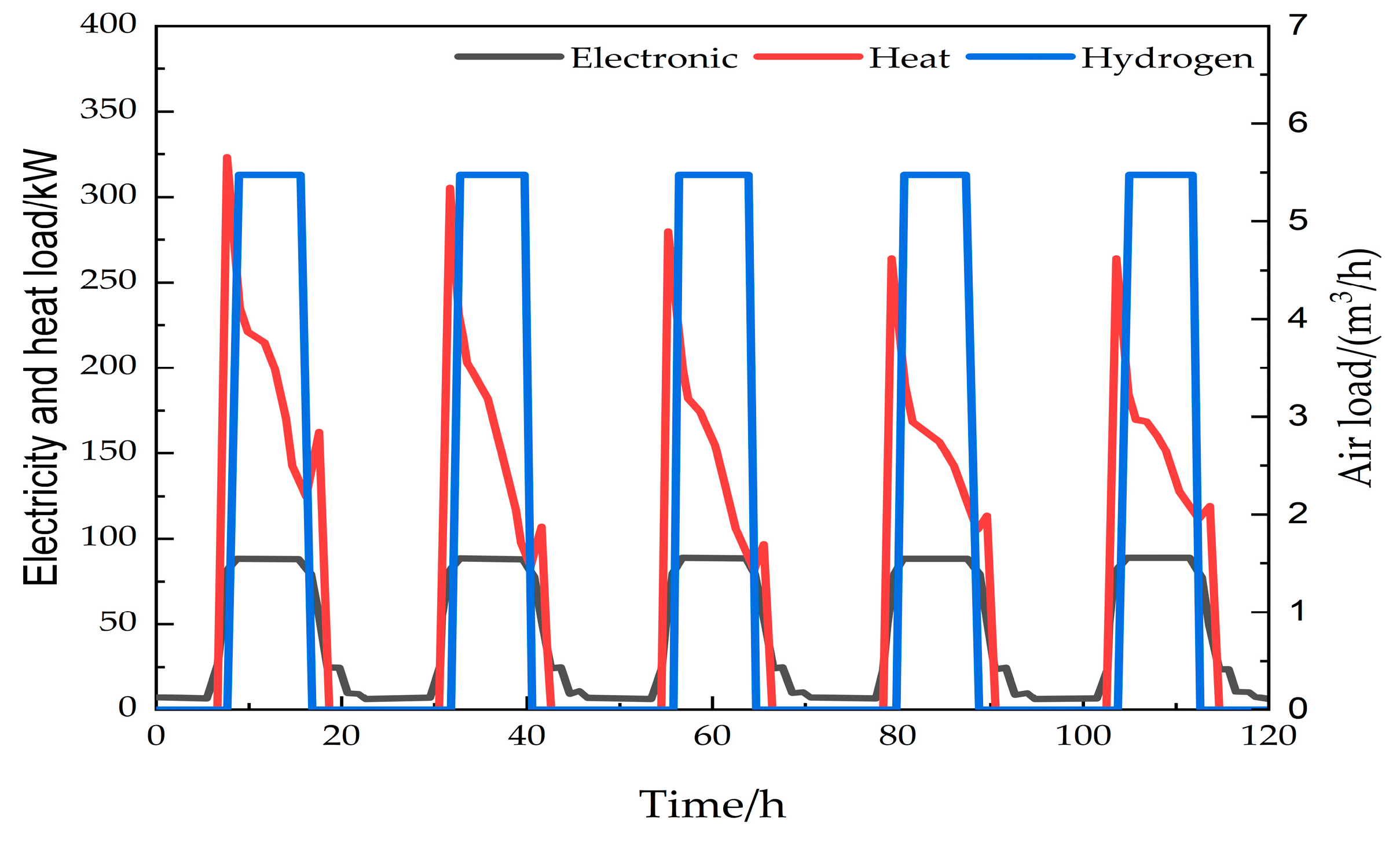
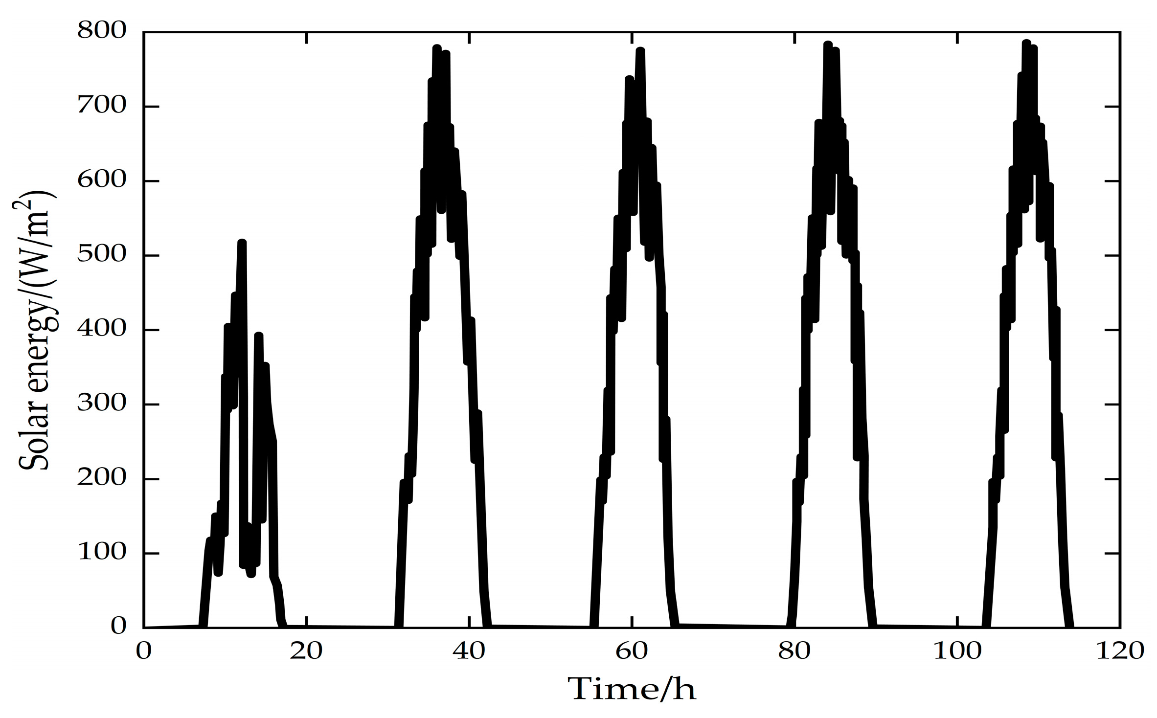
5.1. Arithmetic Conditions

In order to verify the validity and reliability of the constructed model, data from a typical winter’s day in a northern industrial park were selected for our simulation. Since carrying out the optimization calculation for a given year hour-by-hour (a total of up to 8760 h) is highly complicated, five winter working days in January with a large heat load and a time scale of 1 h were used in our simulation to optimize and derive the optimal capacity rationing and responsive scheduling strategies for the various pieces of equipment in the system. The load profile is shown in Figure 3. According to the method described by the authors of [28], the variation in solar radiation energy over time during the simulation cycle can be calculated as shown in Figure 4, which shows that the first day is cloudy with insufficient solar radiation energy and that the remaining four days are sunny with more sufficient solar radiation energy, which more comprehensively reflects the actual weather conditions.

5.2. Analysis of Optimization Results

Using the above models and algorithms, optimization calculations were carried out in MATLAB 2020b software, and the optimal capacity distribution for each piece of equipment in the system was obtained, as shown in

Table 2. System equipment capacity optimization results.

Equipment	Unit	Capacity
PV	m2	487.75
RSOC	kW	279.07
SOEC	m3/h	121.23
HE	kW	350.22
CHP	kW	17.38
Grid	kW	465.28
BT	kW·h	1314.02
MHR	kW·h	252.74
HT	kg	117.78

. The unit prices of electricity, heat, and gas are shown in Figure 5, and it can be seen that the optimized IES unit prices of electricity, heat, and hydrogen are 0.4628 ¥/(kW·h), 0.02 ¥/(kW·h), and 0.51 ¥/m³, respectively, whereas the local prices of industrial and commercial electricity, non-residential heat, and hydrogen are 0.7704 ¥/(kW·h), 0.21 ¥/(kW·h) and 1.98 ¥/m³.

In comparison, the unit prices of electricity, heat, and hydrogen are reduced by 39.9%, 90.5%, and 74.2%, respectively. Since the system uses the waste heat generated by the RSOC in SOFC operation mode to satisfy the heat load, the heat unit price of the system is greatly reduced.

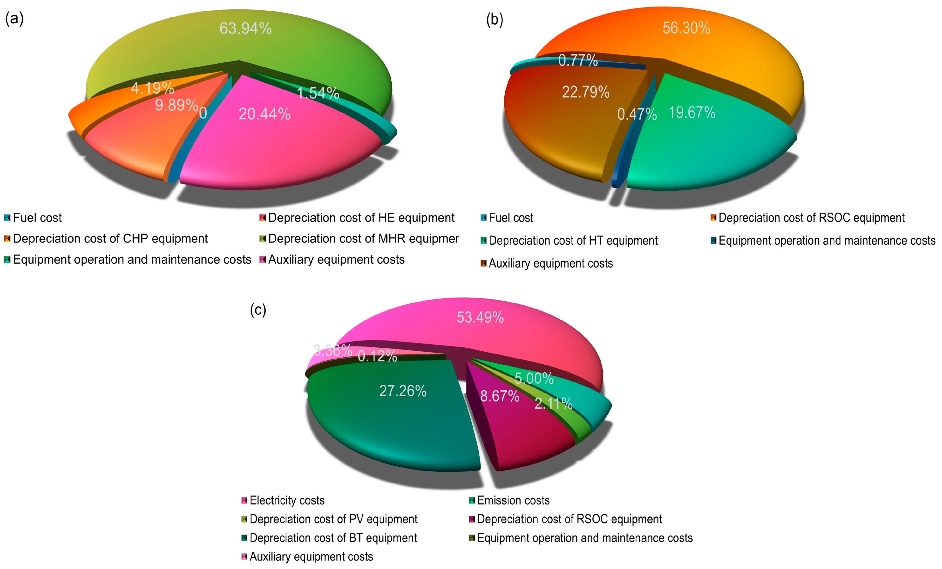
5.2.1. Analysis of System Cost Composition

The system cost composition under the optimal capacity ratio is shown in Figure 6. Under the optimal capacity ratio condition, the cost of the thermal subsystem is mainly spent on the MHR, and the cost of the gas subsystem is mainly spent on the RSOC, so lowering the equipment costs of MHRs and RSOCs can effectively improve the economy of the IES. In the electronic subsystem, the electricity cost of the grid accounts for more than 50% of the total cost, while the PV component does not consume extra costs once it is built, so increasing the utilization rate of PV energy in the IES can also improve the economy of the system.

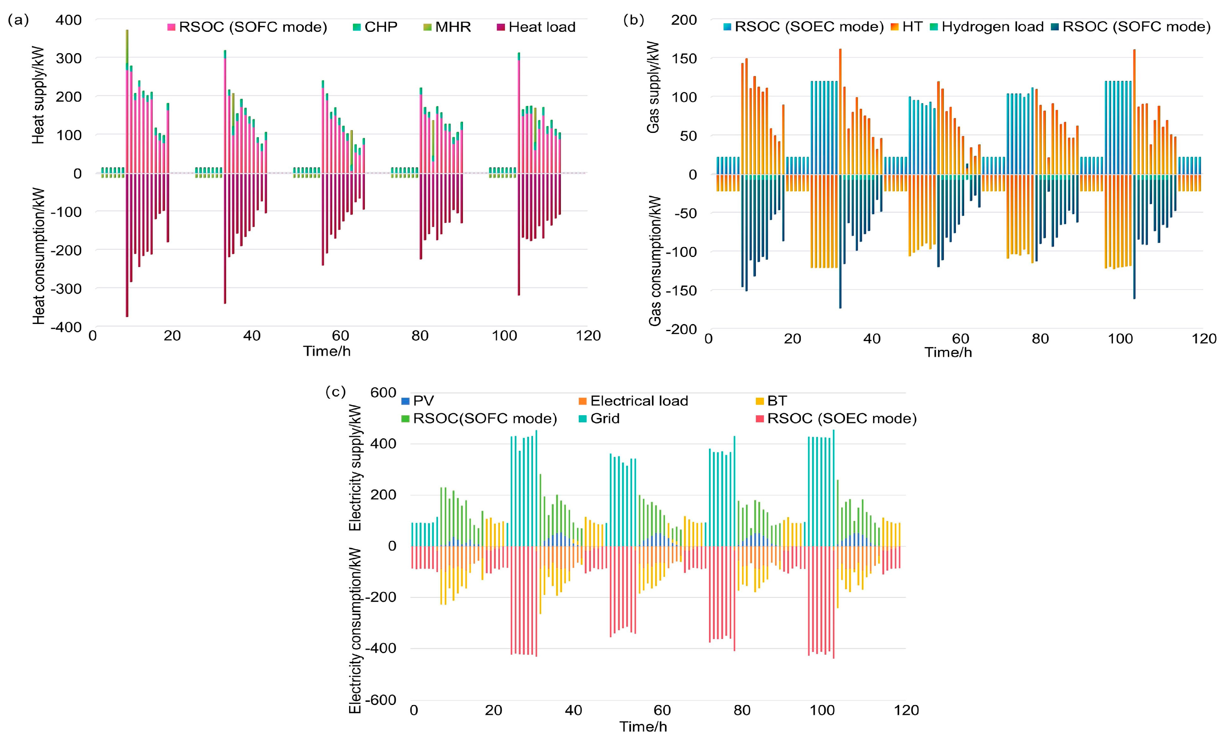
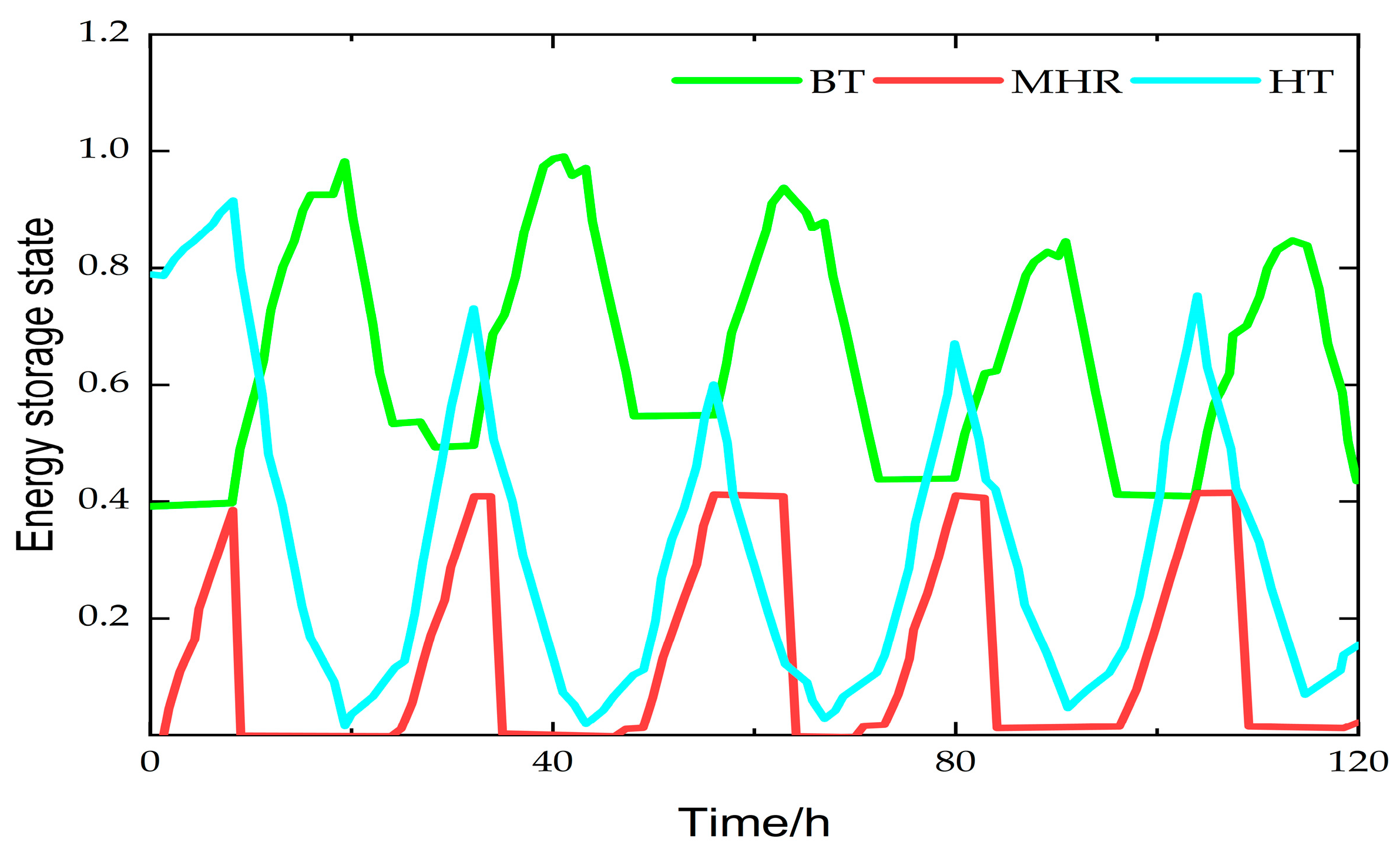
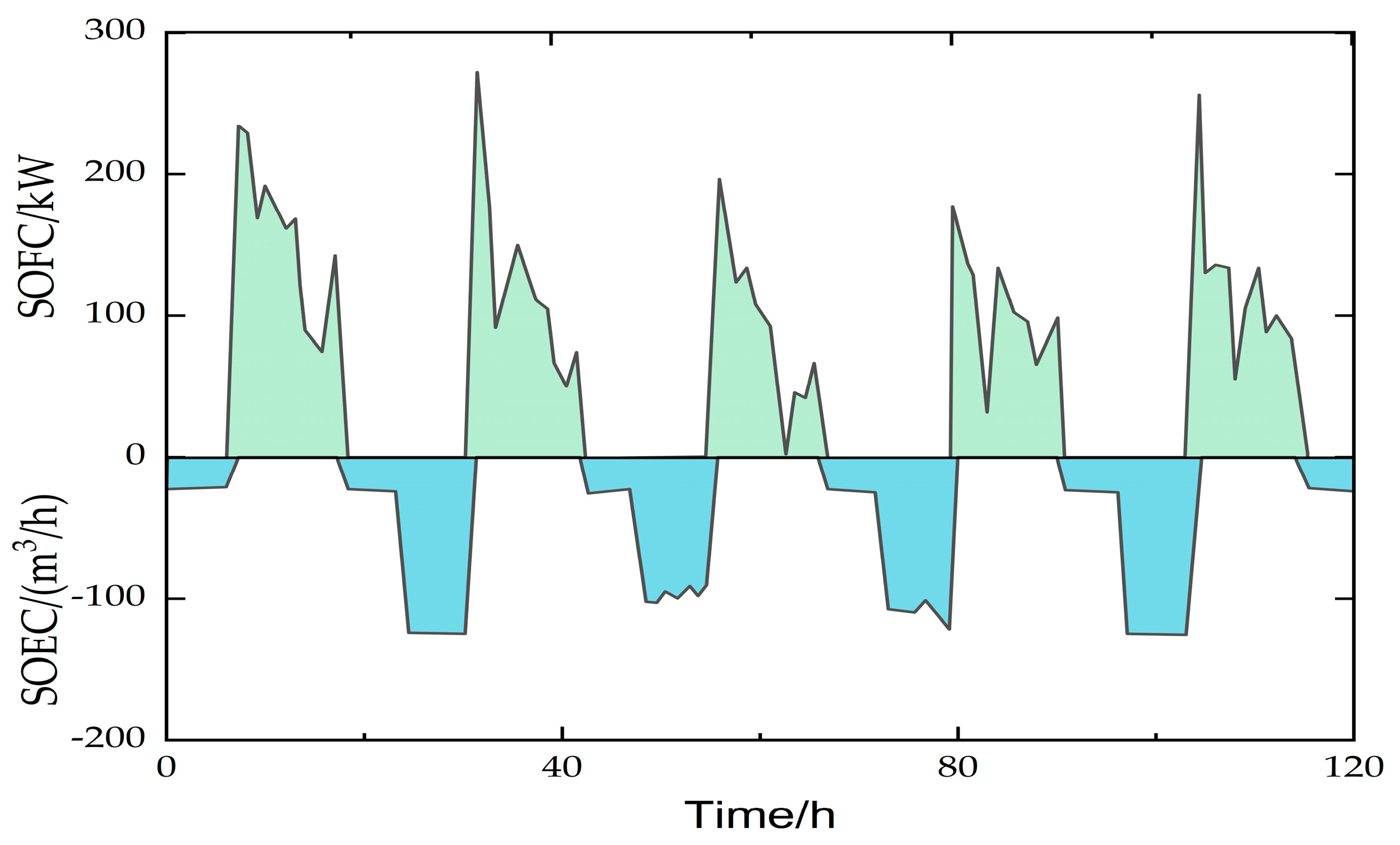
5.2.2. Analysis of System Scheduling Strategies

Figure 7 shows the time-by-time heat, gas, and power scheduling strategies for five working days under the optimal capacity ratio of the system. From Figure 7a, it can be seen that in the nighttime low-heat period, the heat load is mainly satisfied by the CHP, and the excess heat generated exists in the multi-stage storage heaters; in the daytime peak heat period, the waste heat generated by the RSOC satisfies most of the heat load, and the insufficient heat is supplemented by the MHR and CHP. It can be seen from Figure 7b that most of the hydrogen produced by the RSOC in SOEC operation mode is consumed in the SOFC operation mode at the RSOC, which shows that the RSOC is more frequently used as an energy conversion device in the system. It can be seen from Figure 7c that, during the daytime, together, the RSOC and PV component satisfy all the electrical loads and charge the excess electrical energy into the battery for backup; at nighttime, both the RSOC and PV component stop working, the electrical loads are satisfied by the power stored in the battery, and the insufficient power is replenished by the power grid.

The system’s heat supply is equal to heat consumption; its gas supply is equal to gas consumption, and the power supply is equal to the power consumption at any moment, as shown in Figure 7, indicating that the computational model we used satisfies the physical constraints of the system and basically realizes the process of the actual one.

Figure 8 illustrates the energy storage status curves for the battery, the storage heaters, and the hydrogen storage tank, and it can be seen that all three types of energy storage devices are used frequently. The battery basically undergoes one complete charge/discharge cycle per day, always storing part of the daytime power to supply power for the nighttime load demand. This is due to the high thermal load of the system during the daytime and the fact that the system is in FTL operation mode.

As shown in Figure 9, the RSOC is always in SOFC mode during the daytime in order to meet the thermal load of the system, and the excess power generated is charged into the battery. At the same time, the PV component works only during the daytime, and the excess power generated is also charged into the battery. At night, the RSOC is in the SOEC mode and needs to utilize the power stored in the battery during the day to electrolyze hydrogen, which sometimes depletes the battery to the set maximum discharge depth of 0.4. Insufficient power is replenished by the power grid. The storage heaters were not filled during the 5-day simulation, always storing a small amount of heat at night and releasing it during the day to cut down on the daytime heat peak. Regarding the hydrogen storage tank, a certain amount of hydrogen is set to be stored in the tank initially, and it can be seen from Figure 8 and Figure 9 that the RSOC is in the SOEC mode at night to produce hydrogen by electrolysis. The hydrogen produced is stored in the tank and released during the daytime for the RSOC in the SOFC mode to use to meet the required hydrogen load of the system.

5.2.3. Comparative Analysis

In this study, Multi-Objective Optimization (MOO) [29] and mixed-integer linear programming (MILP) [30] were selected to facilitate a comparison between these methods and our proposed one. The former is used to find a set of solutions which find an optimal balance between different objectives, while the latter minimizes a linear objective function under linear constraints while requiring some or all of the variables to be integer-valued. All experiments were carried out in MATLAB, and the YALMIP R20200930 toolbox [31] and the commercial software Gurobi 10.0 [32] were also used. The optimization results are shown in

Table 3. Comparative analysis.

Optimization Methods	Energy Unit Price Reduction Rate
	Electricity	Heat	Hydrogen
MOO	36.2%	85%	73.9%
MILP	39.6%	87.3%	72.1%
RCA + SQP	39.9%	90.5%	74.2%

, where it can be seen that the optimization method proposed in this paper is superior to the other two methods, validating its effectiveness.

6. Conclusions

In this paper, a capacity matching optimization and scheduling strategy model for a multi-energy flow integrated energy system with the objective of maximizing the economic benefits of electricity, heat, and gas is proposed. The model was optimized and solved using an RCA combined with SQP to obtain the optimal capacity matching of each device in the system and the optimal scheduling strategies for the electricity, heat, and gas energy in the simulation cycle in order to ensure that the system has the lowest energy cost while satisfying the load. Based on our study, the following conclusions were drawn:

(1)

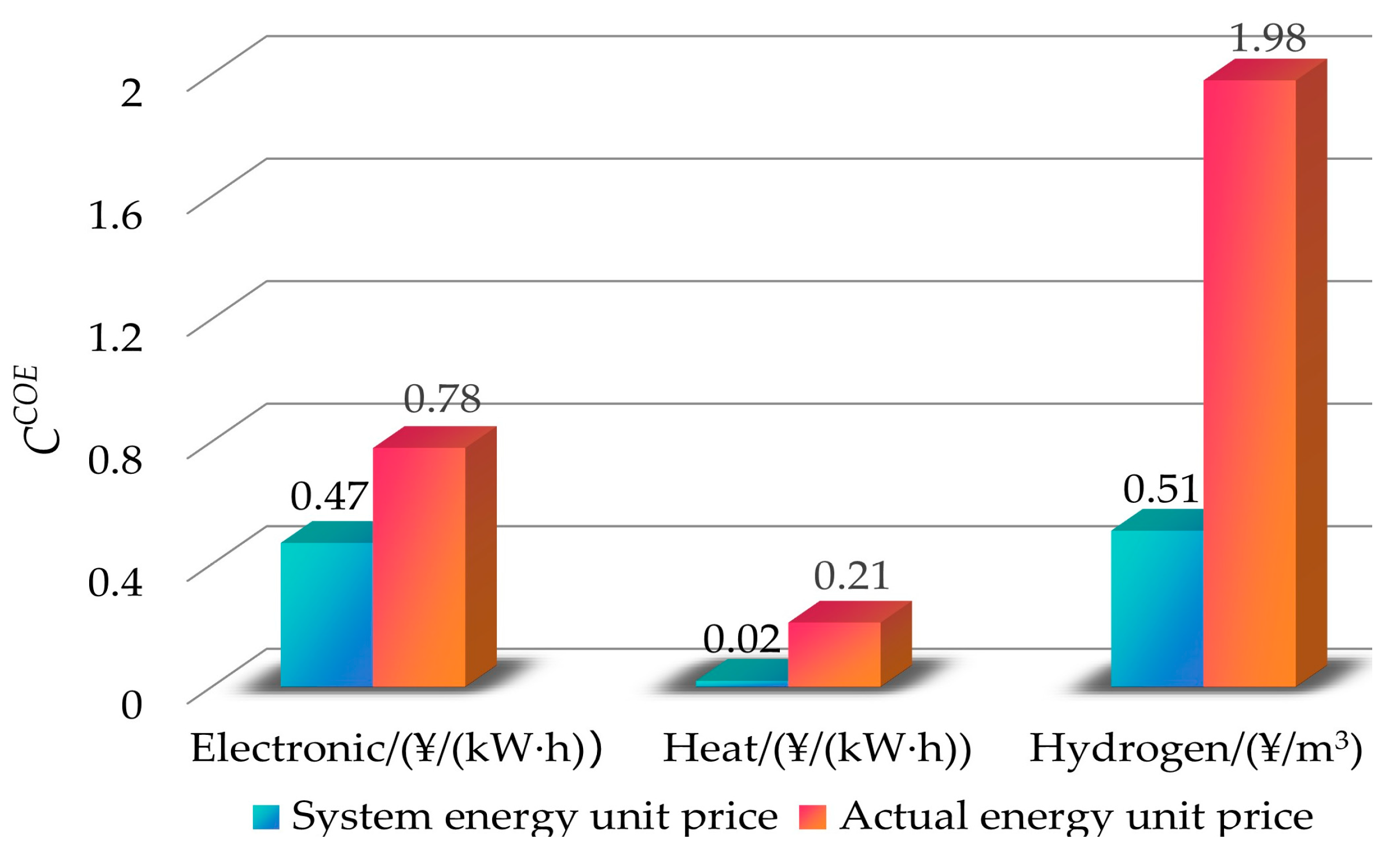
Compared with the current market energy unit price, the utilization of this integrated energy system can reduce the unit prices of electricity, heat, and hydrogen by 39.9%, 90.5%, and 74.2%, respectively, effectively improving the economy of the system.

(2)

Through analyzing the system cost components, it can be seen that reducing the equipment costs associated with MHRs and RSOCs and improving the utilization rate of solar cells can effectively improve the system from an economic standpoint.

(3)

This model was solved using RCA and SQP algorithms, which can adapt to energy systems of different sizes and complexities and provide a reference for the construction of integrated energy systems.

In addition, the system’s design can be optimized when the grid is supplied with electricity without considering the impact of time-sharing tariffs. In the future, the proposed model could be applied in different time periods with refinement.

References

1. Wang, Q.; Wang, C.M.; Xie, N. Hybrid CVaR-IGDT planning model for regional integrated energy system expansion. Grid Technol. 2020, 44, 505–515. [Google Scholar] [CrossRef]
2. Zhang, X.-d.; Ren, J.; Wang, P. Research on key technology of network source coordination in energy internet environment. Inf. Technol. 2021, 12, 100–105. [Google Scholar] [CrossRef]
3. Zong, X.; Yuan, Y.; Wu, H. Multi-Objective Optimization of Multi-Energy Flow Coupling System with Carbon Emission Target Oriented. Front. Energy Res. 2022, 10, 877700. [Google Scholar] [CrossRef]
4. Lingmin, C.; Jiekang, W.; Fan, W. Energy flow optimization method for multi-energy system oriented to combined cooling, heating and power. Energy 2020, 211, 118536. [Google Scholar] [CrossRef]
5. Bazdar, E.; Sameti, M.; Nasiri, F. Compressed air energy storage in integrated energy systems: A review. Renew. Sustain. Energy Rev. 2022, 167, 112701. [Google Scholar] [CrossRef]
6. Zhao, J.; Chen, L.; Wang, Y. A review of system modeling, assessment and operational optimization for integrated energy systems. Sci. China Inf. Sci. 2021, 64, 191201. [Google Scholar] [CrossRef]
7. Tian, H.; Zhao, H.; Liu, C. Iterative linearization approach for optimal scheduling of multi-regional integrated energy system. Front. Energy Res. 2022, 10, 828992. [Google Scholar] [CrossRef]
8. Xu, G.; Guo, Z.X. An incentive-based integrated demand response optimization strategy considering multidimensional response characteristics of users in multistate energy systems. Chin. J. Electr. Eng. 2023, 43, 9398–9411. [Google Scholar] [CrossRef]
9. Ma, D.; Gao, H.J.; Zhang, J.L. Coordinated optimization of integrated electricity-gas energy system considering wind power uncertainty. Smart Power 2022, 50, 33–40. [Google Scholar]
10. Zhang, W.D.; Liu, Z.K. Multi-neural network based forecasting model for user-side cooling and heating loads in integrated energy systems. Microcomput. Appl. 2023, 39, 210–214. [Google Scholar]
11. Wang, Y.L.; Xiang, H.; Li, S.C. Operation optimization of regional integrated energy system considering coupling characteristics of cooling, heating and power cogeneration system. Sci. Technol. Eng. 2023, 23, 7787–7797. [Google Scholar]
12. Wang, J.; Jin, Y.; Zheng, J. Optimal quantity, location and capacity allocation of the additional renewable energy stations in a large-scale district heating system and comprehensive case analyses. Energy Convers. Manag. 2023, 284, 116975. [Google Scholar] [CrossRef]
13. Ahmad, M.S.; Ali, M.S.; Abd Rahim, N. Hydrogen energy vision 2060: Hydrogen as energy Carrier in Malaysian primary energy mix—Developing P2G case. Energy Strategy Rev. 2021, 35, 100632. [Google Scholar] [CrossRef]
14. Feng, X.; Yang, C.; Liang, C.Y. Numerical simulation study of reversible solid oxide fuel cell performance. Propuls. Technol. 2020, 41, 2630–2640. [Google Scholar] [CrossRef]
15. Pianko-Oprych, P.; Hosseini, S.M. Dynamic analysis of load operations of two-stage SOFC stacks power generation system. Energies 2017, 10, 2103. [Google Scholar] [CrossRef]
16. Lu, Y.; Li, J.; Souamy, L. Model Analysis on Hydrogen Production by Hybrid system of SOEC and Solar Energy. Eng. Lett. 2017, 25, 1–7. [Google Scholar]
17. Rispoli, N.; Vitale, F.; Califano, F. Constrained optimal design of a reversible solid oxide cell-based multiple load renewable microgrid. J. Energy Storage 2020, 31, 101570. [Google Scholar] [CrossRef]
18. Wang, Y.; Wang, W. Research on the Control Strategy of Urban Integrated Energy Systems Containing the Fuel Cell. Processes 2023, 11, 1584. [Google Scholar] [CrossRef]
19. Dursun, B. Determination of the optimum hybrid renewable power generating systems for Kavakli campus of Kirklareli University, Turkey. Renew. Sustain. Energy Rev. 2012, 16, 6183–6190. [Google Scholar] [CrossRef]
20. Zhang, C.; Chen, H.; Shi, K. A multi-time reactive power optimization under interval uncertainty of renewable power generation by an interval sequential quadratic programming method. IEEE Trans. Sustain. Energy 2018, 10, 1086–1097. [Google Scholar] [CrossRef]
21. Wang, Z.G.; Yang, X.G.; Wang, Y.Z. Strategy analysis and optimal design of multi-energy coupled cooling, heating and power system. Therm. Power Eng. 2019, 34, 9–14+44. [Google Scholar] [CrossRef]
22. Zhang, X.; Li, M.; Ge, Y. Techno-economic feasibility analysis of solar photovoltaic power generation for buildings. Appl. Therm. Eng. 2016, 108, 1362–1371. [Google Scholar] [CrossRef]
23. Wang, L.L.; Wu, H.B.; Zhou, Y.Y. Optimized allocation of integrated energy system based on energy supply reliability. J. Sol. Energy 2021, 42, 395–400. [Google Scholar] [CrossRef]
24. Wu, K.H.; Wu, J.; Feng, L. Study on optimal dispatching strategy of regional energy microgrid. Math. Probl. Eng. 2020, 2020, 2909023. [Google Scholar] [CrossRef]
25. Wang, X.X.; Lei, Y.; Zhang, T. Segmented optimal scheduling of hydrogen-containing energy storage microgrid based on photovoltaic power generation prediction. Sci. Technol. Eng. 2023, 23, 8218–8226. [Google Scholar]
26. Zhong, L.; Zhang, L.; Xu, H. Simulation of SOFC cogeneration system application. J. Power Eng. 2015, 35, 846–852. [Google Scholar]
27. Sun, Z.H.; Hu, J.P.; Qi, H. Wind power consumption strategy of regional integrated energy system taking into account the integrated demand response of ground source heat pump and electric heat. Electromech. Eng. Technol. 2023, 52, 235–239+265. [Google Scholar]
28. Gong, J.; Li, C.; Wasielewski, M.R. Advances in solar energy conversion. Chem. Soc. Rev. 2019, 48, 1862–1864. [Google Scholar] [CrossRef] [PubMed]
29. Wei, H.; Lee, F.; Hu, C. MOO-DNAS: Efficient neural network design via differentiable architecture search based on multi-objective optimization. IEEE Access 2022, 10, 14195–14207. [Google Scholar] [CrossRef]
30. Anstreicher, K.M. Testing copositivity via mixed–integer linear programming. Linear Algebra Appl. 2021, 609, 218–230. [Google Scholar] [CrossRef]
31. Ravat, A.K.; Dhawan, A.; Tiwari, M. LMI and YALMIP: Modeling and optimization toolbox in MATLAB. In Proceedings of the Advances in VLSI, Communication, and Signal Processing: Select Proceedings of VCAS 2019, Allahabad, India, 21–23 October 2019; Springer: Singapore, 2021; pp. 507–515. [Google Scholar] [CrossRef]
32. Muley, V.Y. Mathematical linear programming to model microRNAs-mediated gene regulation using Gurobi optimizer. In Modeling Transcriptional Regulation; Springer: Berlin/Heidelberg, Germany, 2021; pp. 287–301. [Google Scholar] [CrossRef]
Figure 1. Multi-energy flow integrated energy system.
Processes 12 00628 g001
Figure 2. Flowchart of the solution algorithm.
Processes 12 00628 g002
Figure 3. Load demand.
Processes 12 00628 g003
Figure 4. Solar radiation curve over the simulation period.
Processes 12 00628 g004
Figure 5. System energy cost optimization results.
Processes 12 00628 g005
Figure 6. System cost components with optimal capacity ratios. (a) Cost components of thermal subsystems; (b) cost components of the gas subsystem; (c) cost components of electronic systems.
Processes 12 00628 g006
Figure 7. System scheduling strategy under optimal capacity rationing. (a) System time-by-time heat supply strategy; (b) system time-by-time gas supply strategy; (c) system time-by-time power supply strategy.
Processes 12 00628 g007
Figure 8. Energy storage state curve.
Processes 12 00628 g008
Figure 9. RSOC operation status curve.
Processes 12 00628 g009