Soft Sensor Modeling Method Considering Higher-Order Moments of Prediction Residuals

Abstract

Traditional data-driven soft sensor methods can be regarded as an optimization process to minimize the predicted error. When applying the mean squared error as the objective function, the model tends to be trained to minimize the global errors of overall data samples. However, there are deviations in data from practical operation, in which the model performance in the estimation of the local variations in the target parameter worsens. This work presents a solution to this challenge by considering higher-order moments of prediction residuals, which enables the evaluation of deviations of the residual distribution from the normal distribution. By embedding constraints on the distribution of residuals into the objective function, the model tends to converge to the state where both stationary and deviation data can be accurately predicted. Data from the Tennessee Eastman process and an industrial cracking furnace are considered to validate the performance of the proposed modeling method.

1. Introduction

In modern chemical processes, quality-related variables are important indicators for process monitoring, control, and optimization [1], while they are usually hard to measure in real time because of both economic constraints and instrument availability [2,3]. Because of this concern, soft sensor techniques are developed to achieve real-time estimation of key quality variables by using easy-to-measure process variables [4]. Generally, soft sensor methods can be categorized into two groups: model-based and data-driven soft sensor methods [5]. The former are built based on the physicochemical governing equations of the processes [6]. However, these governing equations are usually obtained under ideal assumptions, which makes it difficult to apply them to real processes under very complex and non-ideal conditions [7].

With the widespread utilization of distributed control systems (DCSs), an enormous number of process data are collected and stored, which greatly facilitates the development of data-driven soft sensors. Benefitting from the sufficient underlying process information captured from process data, data-driven soft sensor models have made rapid progress in obtaining more objective and accurate estimations [8]. Typical data-driven soft sensor methods include ordinary least squares (OLS), partial least squares (PLS), principal component regression (PCR), least absolute shrinkage and selection operator (Lasso), relevance vector machine (RVM), support vector regression (SVR), and artificial neural network (ANN). Among them, OLS is the simplest type of data-driven soft sensor method, which assumes that the key quality variables are a linear combination of easy-to-measure variables [9]. However, there is multicollinearity among industrial process variables. Therefore, PCR and PLS are proposed to solve this problem [10]. In addition, Lasso and RVM are also commonly applied methods to eliminate multicollinearity which are mainly used for feature selection by sparsifying the parameters. On this basis, Fujiwara et al. integrated nearest correlation spectral clustering and group Lasso and proposed a new correlation-based variable selection method to further improve the estimation performance of the soft sensor model [11]. Urhan et al. proposed an RVM-based adaptive learning method to be applied to nonstationary or drift processes [12]. Considering that modern chemical processes are commonly nonlinear, several nonlinear methods, such as kernel PCR, kernel PLS, and SVR, are utilized in the modeling of soft sensors [13,14,15]. With the rapid development of ANN over the past few years, ANN-based soft sensor methods have been developed to extract nonlinear correlations among process variables [16]. Moreover, a few variants of ANN, such as long short-term memory (LSTM) networks, convolutional neural network (CNN), etc., are also used to establish soft sensor models to capture the dynamic features of industrial processes [8,17,18].

Data-driven soft sensor methods not only can be used for real-time estimation of critical quality variables but can also be applied in the field of fault detection [19]. In statistics, when the relationship among the easy-to-measure variables and the key quality variables can be accurately expressed by a soft sensor model, the prediction residuals should be regarded as a random error, which should conform to the normal distribution [20]. Several fault detection methods based on the idea of residual generation have been proposed [18,21,22]. Soft sensor models are applied to generate residuals, which satisfy the Gaussian distribution data assumptions required by monitoring statistics such as Hotelling’s T² and Q [22]. In addition, the early detection of faults can also be achieved by monitoring changes in residual statistical indicators [23]. Conventionally, the statistics used for fault detection are up to the fourth-order moments [24]. Among them, mean and variance are commonly used first-order and second-order statistics, respectively, which presuppose that the data obey a normal distribution [25]. Higher-order moments are utilized to capture deviations from the normal distribution of data under normal conditions [26,27]. It needs to be emphasized again that the residual-based fault detection model is established on the premise that an accurate soft sensor model can be obtained. Therefore, soft sensor modeling is the crucial step.

Although the modeling methods used in the above soft sensors are different, the study of their modeling process shows that it is essentially an optimization process. The optimal parameters of the model are obtained by using the collected labeled data, which minimizes the error between the measured and prediction values of the key quality variables. Mean square error (MSE) and mean absolute error (MAE) are two common absolute error measurement methods, which are widely applied in the modeling process of data-driven soft sensors as the minimization objective function [28]. In addition, mean absolute percentage error (MAPE), as a measure of relative error, is often applied to forecasting modeling in the economic field [29]. However, the above evaluation indicators are used to average the errors [30]. Willmott et al. demonstrated that the average of the error has no consistent relationship with the error of a single sample, which means that the MSE, MAE, or MAPE of a model can still provide a good result even though the model has poor prediction performance on a few data samples [31]. Because the error information of all samples is condensed into a single value by an evaluation index, it cannot reflect the variations in all errors [32]. Using these evaluation indicators as the objective function does not ensure better prediction for all samples.

In actual industrial processes, a process is usually required to operate steadily under pre-set operating conditions. In this case, key quality variables fluctuate around the pre-set values, with a small range. When a fault occurs or a process enters a new operating condition, key quality variables may deviate far from the original data range, which can be defined as “deviation data”. From the essential analysis viewpoint, the data of steady-state processes have a similar distribution range, are numerous, and present a high repetition rate [33]. In contrast, deviation data are fewer and more difficult to obtain [33]. Compared with smooth data samples, human engineers are more concerned about deviations in key quality variables. Therefore, a soft sensor that can accurately predict deviation data samples of key quality variables would have high practical application value [34]. Obviously, it is difficult to achieve accurate prediction for these deviation data samples when traditional error metrics are used as the objective function in the soft sensor modeling process. When deviation data samples cannot be accurately predicted by the soft sensor model, the prediction residuals of the deviation data samples will be much larger than other data samples, which makes the overall prediction residuals of the model no longer conform to the normal distribution. In other words, the relationship among variables cannot be described by the soft sensor model, assuming that the residuals are random invalid errors. Truncation and logarithmic transformation are two common methods to deal with the non-normal distribution of residuals [35,36]. However, the truncation method requires removing outliers, which may result in partial information loss, and the logarithmic transformation is only suitable for non-negative data [36]. Meanwhile, some robust regression methods have also been proposed to solve the problem of the non-normal distribution of residuals, such as robust locally weighted regression, local M-estimators, and local regression quantiles [37]. But these methods usually require iterative calculations and have high computational complexity. In addition, the above methods do not directly constrain the distribution of the residuals, which means that the residuals obtained may not strictly conform to the normal distribution.

Karunasingha found that when using MSE or MAE as the objective function, the resulting residuals are more consistent with the platykurtic or leptokurtic distributions [38]. In conclusion, it is difficult to achieve normal constraints on the distribution of model residuals when the traditional evaluation indicators are used as objective functions for modeling soft sensor models. If a constraint on the residuals distribution is directly added to the objective function, it should be able to achieve better prediction results. Higher-order moments are effective tools for capturing the statistical characteristics of data, which can be utilized as distribution discrepancy metrics [39]. Wen et al. proposed using higher-order moments as statistical indicators, such as skewness, to capture changes in data distribution characteristics [27]. Li et al. applied higher-order moments to the field of domain adaptation to assess the discrepancy in data distribution between target and source domains [40]. Rezaeianjouybari and Shang proposed to obtain identical features between source and target domains by minimizing the distributional differences among the data features extracted from the target and source domains [41]. According to the above, the discrepancy between the residual distribution and the normal distribution can be evaluated by using higher-order moments. By adding the minimization of the difference between the residuals and the normal distribution to the objective function of the soft sensor model, the residuals could be more consistent with the normal distribution.

In this work, a soft sensor modeling method considering the higher-order moments of prediction residuals is proposed in this work. There are mainly three contributions of this study, denoted below.

(1) A new soft sensor modeling method is proposed: higher-order moments are employed to evaluate the difference between the residual distribution and the normal distribution, and they are added to the objective function to make the residuals more consistent with the normal distribution.

(2) The proposed soft sensor modeling method is employed to improve ordinary least squares and convolutional neural network, so that the soft sensor models can satisfy the modeling assumption that the residuals are normally distributed random errors and have an accurate estimate for each data sample.

(3) Data from the Tennessee Eastman process (TEP) and an industrial cracking furnace are considered to validate the performance of the proposed method.

The remaining sections of this paper are arranged as follows: First, the basis of the proposed method is briefly introduced in Section 2, followed by the detailed introduction of the proposed soft sensor modeling method in Section 3. In Section 4, the TEP and an industrial cracking furnace are used to evaluate the prediction performance of the proposed method. Finally, conclusions are presented in Section 5.

2. Background

The modeling method proposed in this work is an improvement on existing soft sensors and is not limited to application to a specific soft sensor method. In this paper, OLS and CNN will be employed as examples to introduce the proposed modeling method. As background knowledge, OLS and CNN will be briefly introduced in this section.

2.1. OLS

OLS is a typical mathematical optimization technique used to search for the best-fitting curve or function based on a given set of data samples. It aims to obtain the optimal model parameters by minimizing the sum of squares for the vertical distances from the data points to the fitted curve. Let $(X,Y)$ denote a set of data samples, with $X$ representing easy-to-measure variables and $Y$ representing key quality variables, which can be utilized to establish an OLS model. The mathematical expression of the OLS model can be represented as follows:

$$f(x)=a_1{x}_1+a_2{x}_2+\dots +a_m{x}_m$$

(1)

where $f(x)$ indicates the model prediction value, $x_i$ indicates the easy-to-measure variable, $a_i$ indicates the model parameters, and m is the number of easy-to-measure variables.

The objective function of OLS is as follows:

$$\min \frac{1}{n}{\displaystyle \sum _{i=1}^n{(f{(x)}_i-y_i)}^2}$$

(2)

where $y_i$ is the measured value of the key quality variables ($Y$) and n is the number of samples.

2.2. CNN

CNN is a typical multilayer feed-forward neural network, which was initially applied in the field of image recognition [42,43]. Over the last few years, benefiting from the ability to capture dynamic features from process data, CNN has also been widely employed in the modeling of soft sensors [44,45]. Moreover, strategies such as weight sharing, local connection, and pooling operations greatly reduce the model parameters of CNN, significantly cutting down on training time and difficulty [46].

As shown in Part A of Figure 1, CNN consists of an input layer, convolutional layers, pooling layers, fully connected layers, and an output layer. Time-series data are organized into a two-dimensional data matrix, with the width representing the variables and the length representing time, which is input into the CNN [47]. The convolutional layer is first utilized to extract the dynamic features of the data matrix, and the extracted features are compressed by using the pooling layer. Fully connected layers are applied for a further nonlinear mapping of the extracted features. Then, the prediction value is output by the output layer. The backpropagation algorithm is utilized for CNN training. MSE is a commonly used loss function, and its calculation equation is as follows:

$$Loss=\frac{1}{n}{\displaystyle \sum _{i=1}^n{(f{(x)}_i-y_i)}^2}$$

(3)

Based on the brief introduction of OLS and CNN, it can be found that the essence of a soft sensor is to establish the relationship between easy-to-measure variables and key quality variables using the collected data. The objective of modelling is to minimize the error between the measured and prediction values of the key quality variables, and MSE is a commonly used objective function. However, as discussed in the Introduction section, there is an issue with using MSE as an objective function for soft sensor modeling: it pays more attention to minimizing the error of overall data samples while ignoring the prediction performance on a small number of deviation data samples. In order to address this issue, the objective function of the soft sensor model will be modified in this work to improve the prediction effectiveness on deviation data samples.

3. Soft Sensor Modeling Method Considering the Higher-Order Moments of Prediction Residuals

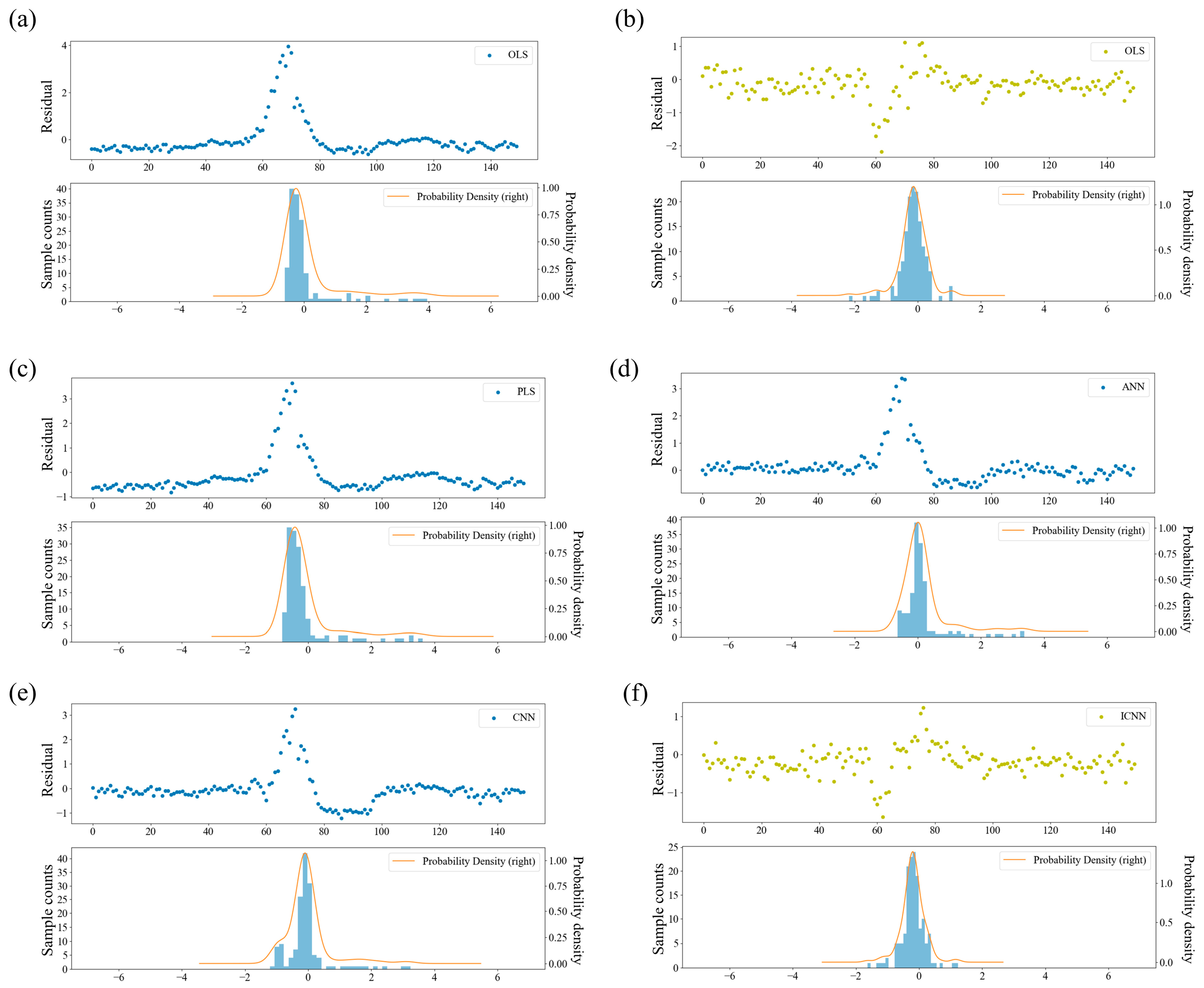
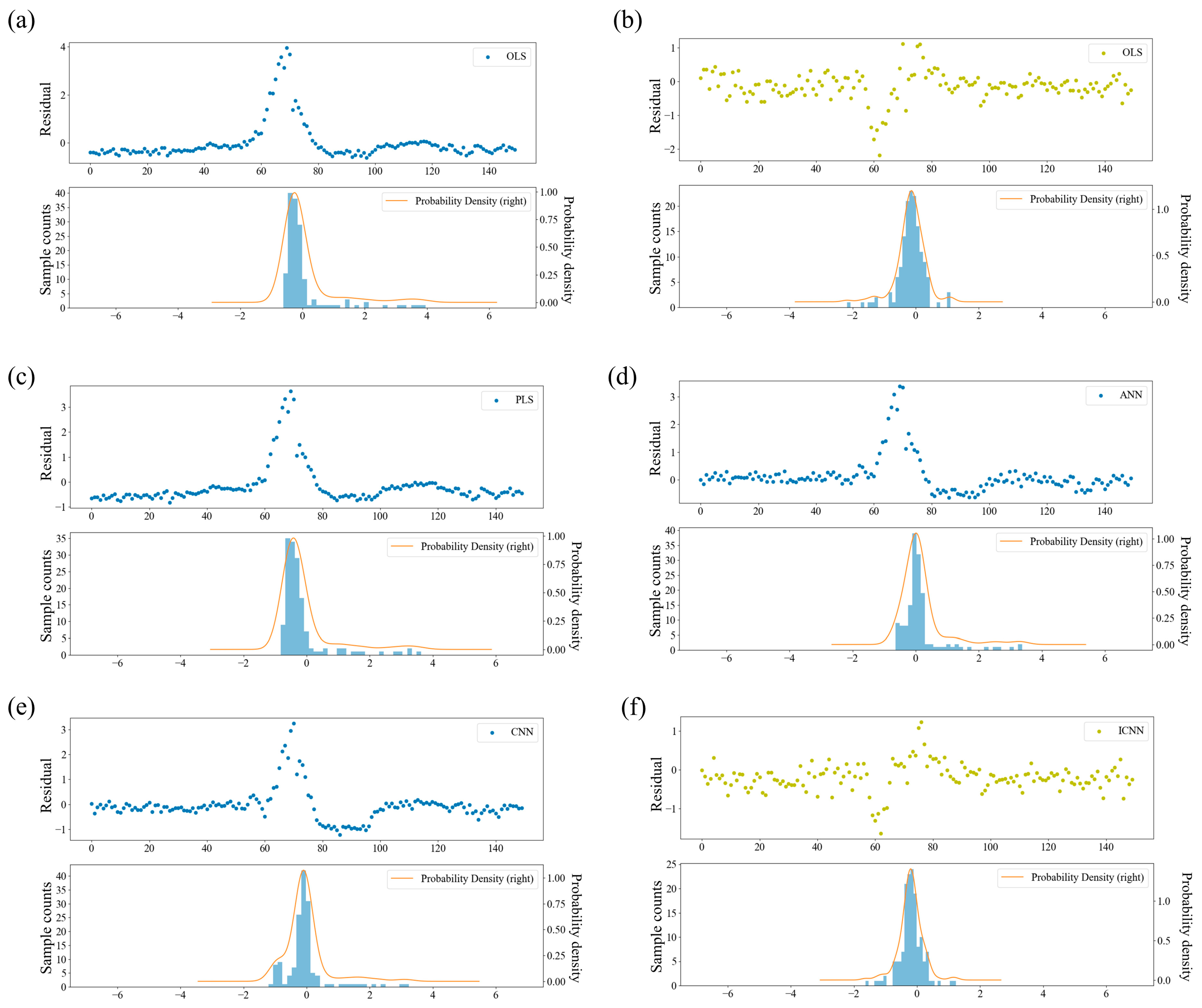
3.1. Residual Analysis

A residual is the difference between the prediction value and the measured value and can be calculated as follows:

$${\epsilon }_i=f{(x)}_i-y_i$$

(4)

In the field of statistics, if the relationship between the input and output variables can be accurately described by a soft sensor model, the residuals should be normally distributed [48].

We use a simulated data set as an example for residuals analysis. Suppose that Model A and Model B are two different soft sensor models. Their prediction results are shown in Figure 2a, and the prediction results of partial data samples are displayed in Figure 2b. As can be seen, for deviation data samples, the prediction performance of Model B is significantly better than that provided by Model A. The same conclusion can be obtained from Figure 2c. The deviation data samples of Model A are far from the symmetry axis, which also indicates that the model is a poor predictor of these samples. In practical industrial processes, human engineers prefer to be able to obtain accurate predictions of deviation samples as opposed to smooth samples, as this can help them identify process anomalies in a timely manner. Obviously, Model B is more popular with human engineers than Model A. However, the MSEs of Model A and Model B are 0.3345 and 0.3724, respectively, which means that Model A is better than Model B from the MSE point of view. Therefore, it is not sufficient to utilize MSE alone to evaluate the performance of a soft sensor model.

The residual distributions of Model A and Model B are illustrated in Figure 2d and Figure 2e, respectively. Clearly, the residuals of Model B conform more closely to a normal distribution compared with those of Model A, owing to the accurate prediction of Model B for the deviation samples. Thus, the evaluation of soft sensor models using the distribution of residuals provides a more remarkable reflection of the prediction performance on deviation samples than MSE. Skewness and kurtosis are two statistical measures that evaluate the characteristics of a data distribution, where skewness is utilized to measure the degree of asymmetry of the distribution. When the residuals conform to a normal distribution, the skewness is 0. The mathematical expression of skewness is shown as follows:

$$Skew=\frac{{\displaystyle \sum _{i=1}^n{({\epsilon }_i-\overline{\epsilon })}^3}}{n{\sigma }^3}$$

(5)

where $\overline{\epsilon }$ and ${\sigma }^2$ represent the mean and variance of the residuals, respectively, which can be calculated by Equations (6) and (7).

$$\overline{\epsilon }=\frac{1}{n}{\displaystyle \sum _{i=1}^n{\epsilon }_i}$$

(6)

$${\sigma }^2=\frac{1}{n}{\displaystyle \sum _{i=1}^n{({\epsilon }_i-\overline{\epsilon })}^2}$$

(7)

Kurtosis is used to measure the degree of peakedness of the distribution. When the residuals conform to a normal distribution, the kurtosis should be 3. It can be calculated by Equation (8).

$$Kurt=\frac{{\displaystyle \sum _{i=1}^n{(\epsilon -\overline{\epsilon })}^4}}{n{\sigma }^4}$$

(8)

The calculations show that the skewness and kurtosis of the prediction residual for Model A are −2.1122 and 19.3092, respectively, and those for Model B are 0.0738 and 2.9585, respectively. This implies that the prediction residuals of Model B are more normally distributed than those of Model A. When the model can accurately describe the relationship among variables, the residuals are only random noise and should conform to the normal distribution. More accurate prediction results for deviation data can be provided by Model B, which shows that Model B can describe the relationship between variables more accurately than Model A, so its residuals are more consistent with the normal distribution. It can be concluded that the prediction residuals are more consistent with a normal distribution when the soft sensor model has better prediction performance on the deviation data. Therefore, a soft sensor modeling method considering the higher-order moments of prediction residuals is proposed in this work. Next, the proposed modeling method is presented in conjunction with OLS and CNN.

3.2. Improved Ordinary Least Squares (IOLS)

The improvement in OLS is mainly reflected in the modification of the objective function. By adding constraints on the distribution of the predicted residuals to Equation (2), a new objective function can be obtained, as shown in Equation (9).

$$\min (\frac{1}{n}{\displaystyle \sum _{i=1}^n{(f{(x)}_i-y_i)}^2}+Ske{w}^2+{(Kurt-3)}^2)$$

(9)

By minimizing the new objective function, the optimal parameters of IOLS can be obtained. In this work, the simulated annealing method is employed to obtain the optimal parameters [49].

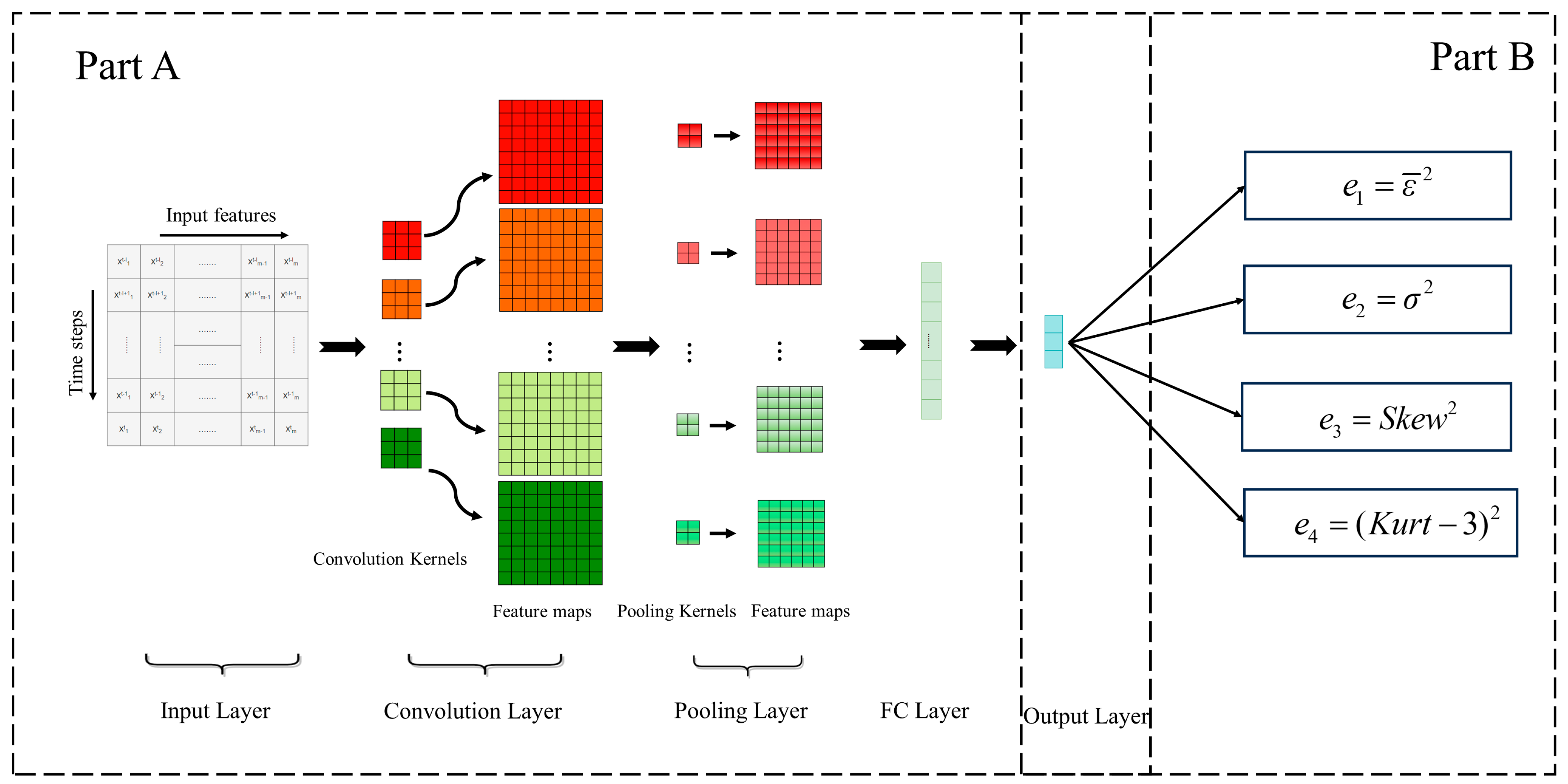
3.3. Improved Convolutional Neural Network (ICNN)

The structure layout of ICNN, as shown in Figure 1, consists of two parts: Part A and Part B, where the former is the traditional CNN. The time-series data are input into the CNN, and output values are obtained through forward propagation, that is, the prediction values of the key quality variable. Then, the output values are employed to calculate the mean, standard deviation, skewness, and kurtosis of the prediction residuals, as shown in Part B of Figure 1. To make the prediction residuals conform to the normal distribution, constraints on the distribution of residuals are embedded in the loss function to train the model. According to the definition of statistics, when the data conform to a normal distribution, their skewness and kurtosis are 0 and 3, respectively. Therefore, constraints on the skewness and kurtosis of the residuals are added to the loss function, as shown in Equation (10). The optimal model parameters of ICNN can be obtained by the back propagation algorithm.

$$Los{s}_{new}=Loss+Ske{w}^2+{(Kurt-3)}^2$$

(10)

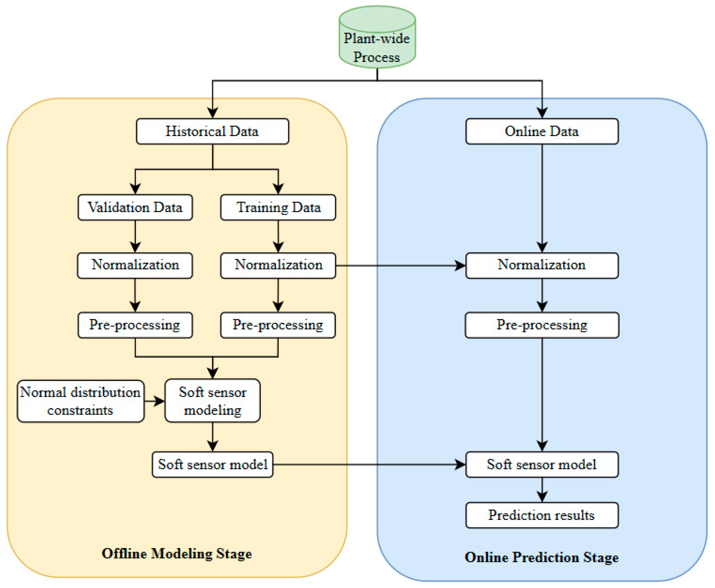
3.4. Framework for Proposed Method

The framework of the proposed soft sensor modeling considering higher-order moments of prediction residuals is presented in Figure 3, which consists of two parts: the offline modeling stage and the online prediction stage.

• Offline modeling stage

Step 1: Historical data collected from the plant are categorized into training data and validation data, ensuring that deviation data samples are contained in both sets.

Step 2: In order to reduce the complexity and time consumption of modeling, the training data are first normalized, and the validation data are scaled using the mean and standard deviation of the training data [50].

Step 3: The normalized data are pre-processed according to the requirements of the model input and then utilized to build a soft sensor model considering the higher-order moments of the prediction residuals, where the training data are utilized to establish the soft sensor model and the validation data are utilized to determine the key parameters to prevent model overfitting.

• Online prediction stage

Step 1: Data collected online are first scaled using the mean and standard deviation of the training data.

Step 2: The normalized data are pre-processed according to the input requirements of the soft sensor model.

Step 3: The pre-processed data are fed to the soft sensor model obtained in the offline modeling stage; then, the output values are inversely normalized to obtain the prediction values.

4. Case Study

To test the capabilities of the proposed modeling method, the improved soft sensor model is applied to the TEP and an ethylene production process. Root mean squared error (RMSE), Mean Absolute error (MAE), mean squared logarithmic error (MSLE), mean absolute percentage error (MAPE), and coefficient of determination (R²) are soft sensor evaluation indicators commonly used to evaluate prediction performance [29,51,52,53,54].

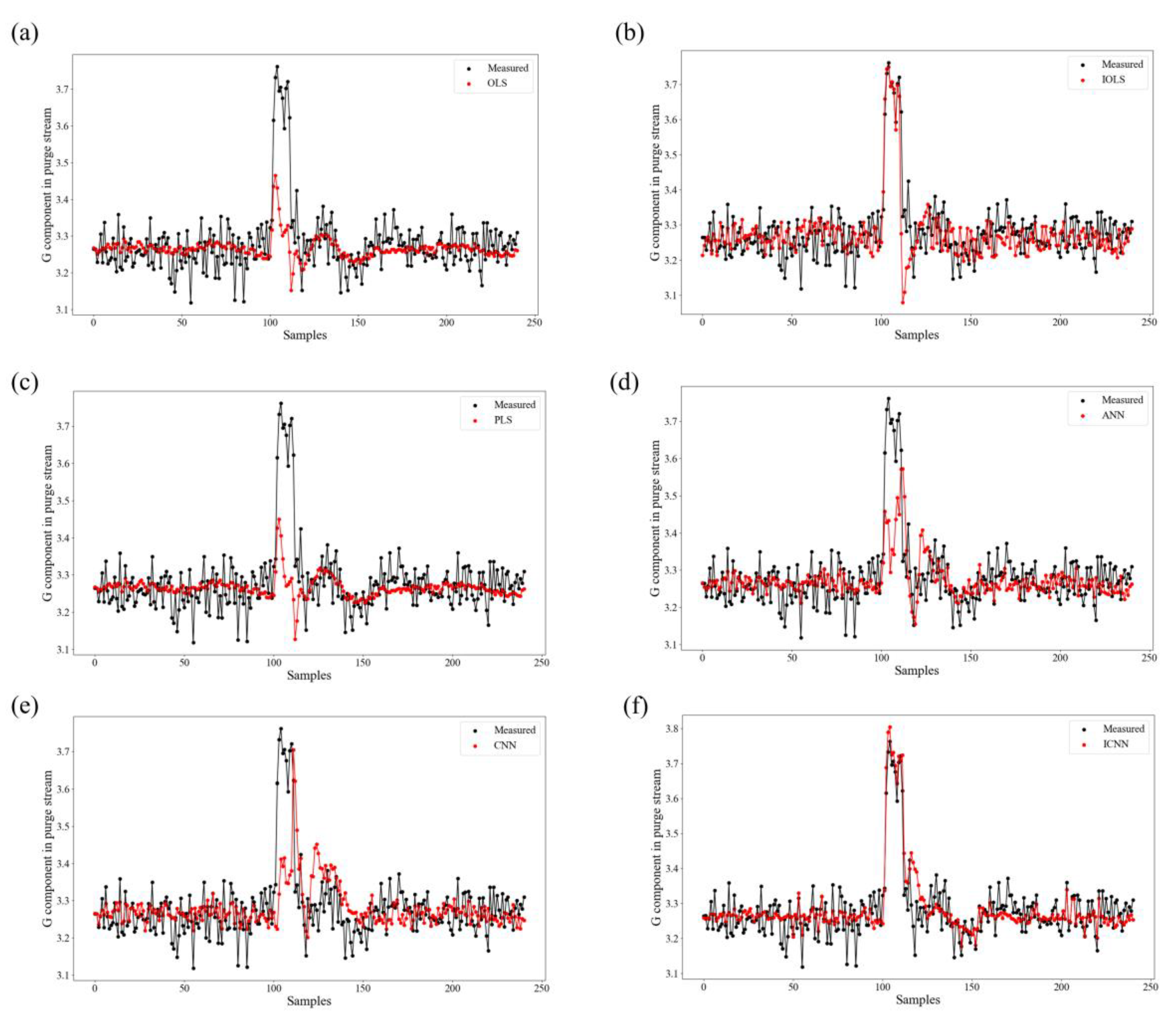
4.1. Tennessee Eastman Process

In previous research studies, the TEP has been frequently applied as a benchmark platform to validate algorithms and evaluate performance [55]. The TEP consists of five process units with 12 manipulated variables and 41 measured variables. Among the measured variables, 19 are composition measurements, which are sampled much less frequently than the other variables. Therefore, in order to monitor the product, it is essential to establish soft sensor models to achieve accurate real-time estimation of these composition measurements. In this work, 33 easy-to-measure variables are used to develop a soft sensor model for the prediction of component G in stream 9. Simulation data are generated by the Simulink version of the TEP [56,57]. The sampling intervals for easy-to-measure variables and component G are set at 1 min and 6 min, respectively. In addition, deviation data samples of component G are generated by introducing deviations into the reactor temperature. For a more intuitive presentation of the generated data, T-SNE is applied for low-dimensional visualization. As shown in Figure 4, the training data, validation data, and test data all contain a small number of deviation data. Using traditional soft sensor modeling methods tends to lead to models with better predictions for most data samples, thereby ignoring the prediction accuracy of the deviation data samples.

According to the methods proposed in Section 3, soft sensor models based on IOLS and ICNN are established, respectively. Furthermore, in order to verify the efficacy of the proposed method, OLS, PLS, ANN, and CNN are also applied for soft sensor modeling. The detailed structures of CNN and ICNN are illustrated in

Table 1. Detailed structures of CNN and ICNN.

Model	Input Dimension	Convolutional Layer	Pooling Layer	Convolutional Layer	FC Layer	Output Layer
CNN	2D matrix	3 (3, 3)	Average pooling	5 (2, 1)	Flatten	1
ICNN	2D matrix	3 (3, 3)	Average pooling	5 (2, 1)	Flatten	1

, form which it can be seen that they are the same, which can be employed to compare the prediction performance of the model after adding normal distribution constraints. The prediction results of these methods are displayed in Figure 5, where the prediction values are represented in red and the measured values are represented in black. From the figure, it can be seen that the prediction values obtained by traditional soft sensor methods using MSE as the objective function cannot fit the true values well, especially for deviation data samples. In contrast, IOLS and ICNN can accurately predict deviation data samples. Meanwhile, as can be seen from

Table 2. Comparison of the prediction results of different soft sensor methods.

	MSE	RMSE	MAE	MSLE	MAPE	R2	Skew	Kurt
OLS	0.0071	0.0845	0.0525	3.65 × 10−4	1.5609	0.2452	−2.2953	7.8330
IOLS	0.0042	0.0648	0.0472	2.29 × 10−4	1.4393	0.5562	−0.9265	4.2023
PLS	0.0080	0.0895	0.0539	4.11 × 10−4	1.6002	0.1521	−2.5255	8.8929
ANN	0.0060	0.0774	0.0502	3.07 × 10−4	1.4979	0.3652	−1.6846	7.1492
CNN	0.0077	0.0879	0.0564	3.97 × 10−4	1.6827	0.1814	−1.7075	6.9167
ICNN	0.0023	0.0487	0.0360	1.29 × 10−4	1.0985	0.7488	0.8395	2.8176

, the MSE, RMSE, MAE, MSLE and MAPE of IOLS and ICNN are lower than the traditional soft sensor methods, which shows that the proposed modeling method can significantly enhance the prediction accuracy of the soft sensor models.

The distributions of the prediction residuals for six different soft sensor models are shown in Figure 6. As can be seen, the prediction residuals of traditional soft sensor methods show a positively skewed distribution, which is caused by the inaccurate prediction of deviation data samples. In contrast, the prediction residuals of OLS and CNN show a symmetric distribution, indicating that they are more consistent with the normal distribution. In addition, as shown in Table 2, the skewness and kurtosis of the prediction residuals of IOLS and ICNN are closer to 0 and 3, respectively, which also indicates that their residuals are more consistent with a normal distribution.

We further explore the effect of different proportions of deviation data in the training data on the prediction performance. The TE process is employed to generate training data sets, which include 0‰, 2‰, 4‰, 6‰, and 10‰ of the deviation data, respectively. Then, soft sensor models based on OLS and IOLS are established. Test data are utilized to verify the established soft sensor models, and the results are shown in

Table 3. The effect of different proportions of deviation data in the training data on the prediction performance.

	MSE	RMSE	MAE	MSLE	MAPE	R2	Skew	Kurt
OLS (0‰)	0.0889	0.2983	0.1023	5.80 × 10−3	2.9280	−8.4157	−4.3791	18.4649
IOLS (0‰)	0.0763	0.2762	0.1022	4.78 × 10−3	2.9435	−7.0721	−4.1892	17.4595
OLS (2‰)	0.0092	0.0958	0.0557	4.70 × 10−4	1.6487	0.0281	−2.7006	9.9766
IOLS (2‰)	0.0043	0.0653	0.0484	2.29 × 10−4	1.4628	0.5492	−0.9236	4.9967
OLS (4‰)	0.0071	0.0846	0.0525	3.65 × 10−4	1.5609	0.2452	−2.2953	7.8330
IOLS (4‰)	0.0042	0.0648	0.0472	2.29 × 10−4	1.4393	0.5562	−0.9265	4.2023
OLS (6‰)	0.0025	0.0497	0.0399	1.35 × 10−4	1.2166	0.7385	0.1788	3.3032
IOLS (6‰)	0.0024	0.0494	0.0383	1.34 × 10−4	1.1708	0.7416	−0.0325	3.1601
OLS (8‰)	0.0024	0.0490	0.0403	1.32 × 10−4	1.2286	0.7451	0.2892	3.1451
IOLS (8‰)	0.0024	0.0490	0.0375	1.32 × 10−4	1.1445	0.7456	−0.0765	3.6916
OLS (10‰)	0.0024	0.0488	0.0391	1.31 × 10−4	1.1947	0.7474	0.2648	3.3319
IOLS (10‰)	0.0024	0.0489	0.0387	1.32 × 10−4	1.1818	0.7468	0.1617	3.6318

. When the training data set does not contain deviation data, neither OLS nor IOLS can provide good prediction results, and the residuals of the models do not conform to the normal distribution. As the training data contain deviation samples, the proposed method can provide better prediction results, mainly because the deviation samples can be accurately predicted. When the proportion of deviation samples in the training data exceeds 6%, both OLS and IOLS can provide better prediction results, and the model residuals are also close to the normal distribution. In summary, when the training data contain fewer deviation data, the proposed soft sensor modeling method is better than the traditional soft sensor method.

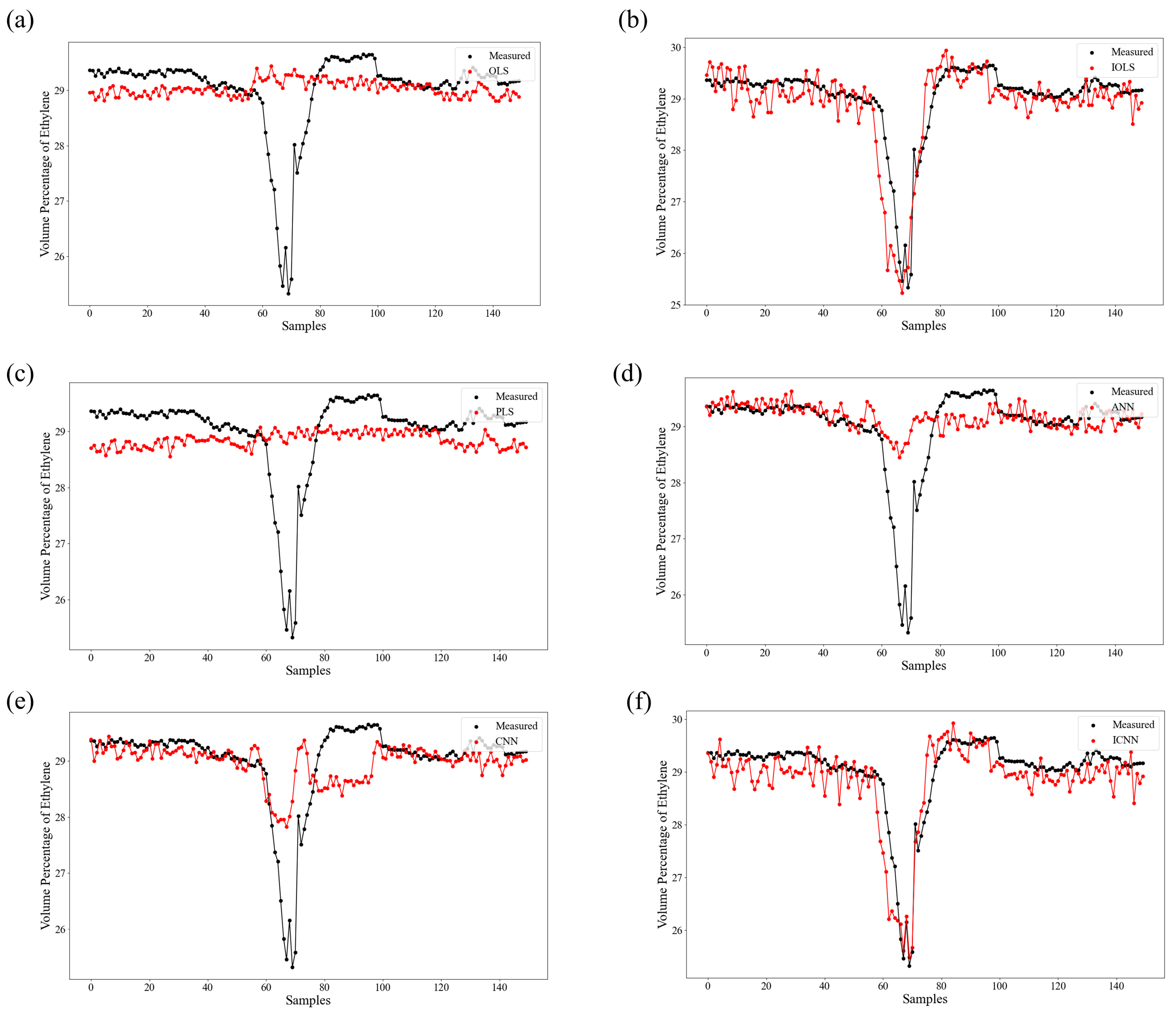
4.2. Industrial Cracking Furnace

Ethylene stands as a pivotal chemical material with significant importance in the realm of petrochemicals. Currently, one of the most widely adopted methodologies for ethylene generation involves the steam cracking of naphtha, serving as a prominent technical pathway. Industrial cracking furnace is the core equipment of this process, where diluted steam and naphtha undergo highly complex cracking reactions to produce olefins, alkanes, and other coproducts. In practice, the volume percentage of ethylene in the cracker outlet composition is a key quality variable of interest to engineers which is hard to measure online. In this work, soft sensor models are established using easy-to-measure variables as illustrated in

Table 4. Process variable information of the cracking furnace.

No.	Description	Unit
x1–x7	Naphtha mass flow rate	kg/h
x8	Naphtha temperature	°C
x9	Naphtha pressure	Mpag
x10–x16	Diluted steam mass flow rate	kg/h
x17	Diluted steam temperature	°C
x18–x23	Crossover section temperature	°C
x24–x29	Crossover section pressure	Mpag
x30, x31	Temperature in furnace A/B side	°C
x32	Fuel gas flow rate	kg/h
x33–x57	Coil outlet temperature	°C
x58–x63	Outlet pressure	Mpag

to estimate the volume percentage of ethylene in real time.

To develop soft sensor models, 2025 sets of data samples for the volume percentage of ethylene and the corresponding easy-to-measure variables are collected. Among them, 1900 data samples are utilized as training data to build the soft sensor model, and 125 data samples are used as validation data to prevent model overfitting. Furthermore, 150 data samples are collected to test the effectiveness of the soft sensor model. Then, soft sensor models based on OLS, IOLS, PLS, ANN, CNN, and ICNN are built, respectively. The detailed structures for CNN and ICNN are illustrated in

Table 5. Detailed structures of CNN and ICNN.

Model	Input Dimension	Convolutional Layer	Pooling Layer	Convolutional Layer	FC Layer	Output Layer
CNN	2D matrix	5 (3, 3)	Average pooling	8 (2, 1)	Flatten	1
ICNN	2D matrix	5 (3, 3)	Average pooling	8 (2, 1)	Flatten	1

. The prediction results are shown in Figure 7 for the six methods on the test data. As can be seen, the predicted curves of OLS and PLS cannot track the true curve. The prediction performance of ANN and CNN is better than that of OLS and PLS, because the nonlinear correlations among variables can be captured by ANN and CNN. However, the above four methods are not effective in predicting deviation data samples near the 60th to 80th samples. The reason is that MSE is used as the objective function in these methods, which makes the modeling process prefer to obtain a model with a better track with the majority of true values, thus ignoring the prediction accuracy of the deviation data samples. In contrast, IOLS and ICNN not only accurately predict smooth samples but also accurately track deviation samples. Therefore, the proposed modeling method is more suitable for practical industrial applications. Human engineers can intervene in advance based on accurate predictions for deviation samples to ensure that the volume percentage of ethylene remains within a preset range.

The MSE, RMSE, MAE, MSLE, MAPE, and R² of the six different methods on the test data are listed in

Table 6. Comparison for the prediction results of different soft sensor methods.

	MSE	RMSE	MAE	MSLE	MAPE	R2	Skew	Kurt
OLS	0.6899	0.8306	0.4671	8.30 × 10−4	1.6747	−0.1599	3.1527	10.0216
IOLS	0.2086	0.4567	0.3123	2.50 × 10−4	1.0896	0.6493	−1.0149	4.9531
PLS	0.6615	0.8133	0.5602	7.93 × 10−4	1.9832	−0.1121	3.1218	10.0271
ANN	0.4801	0.6929	0.3518	5.87 × 10−4	1.2682	0.1928	2.9270	9.9334
CNN	0.4342	0.6590	0.3811	5.24 × 10−4	1.3529	0.2699	2.3434	8.3853
ICNN	0.1721	0.4150	0.3122	1.99 × 10−4	1.0807	0.7105	−0.0981	3.6372

. As can be seen, IOLS and ICNN are better than the traditional methods in all soft sensor evaluation indexes. The prediction performance of ICNN on the test data is superior to that of IOLS. The reason could be that the nonlinear and dynamic features among variables can be captured by ICNN. To further validate the effectiveness of the proposed modeling method, the residuals of the six soft sensor models are analyzed. As shown in Figure 8, the residuals of the traditional soft sensor models represent a positively skewed distribution, while the residuals of IOLS and ICNN show a symmetric distribution. This means that the residuals of IOLS and ICNN are more consistent with the normal distribution than those of traditional soft sensor models. The same conclusion can be obtained from Table 6. The skewness and kurtosis of the predicted residuals for the proposed soft sensor modeling method are closer to 0 and 3, respectively. The results show that by adding constraints on the distribution of the predicted residuals to the objective function, the predicted residuals are made more consistent with the normal distribution, which satisfies the assumption that the prediction residuals should be random errors obeying the normal distribution.

5. Conclusions

In this work, a soft sensor modeling method considering the higher-order moments of prediction residuals is proposed. Different from the traditional modeling methods that use MSE or MAE as the objective function, the constraint on the distribution of the predicted residuals is embedded into the objective function in the proposed method, which leads the model to converge to a state where prediction residuals conform to a normal distribution. The proposed modeling method is employed to improve OLS and CNN. A benchmark process, the TE process, is first utilized to demonstrate the prediction performance of the proposed method; then, an ethylene production process is analyzed to illustrate the applicability of the proposed method to practical industrial processes. Compared with other soft sensor methods, the proposed method provides better prediction results.

References

1. Yuan, X.; Huang, B.; Wang, Y.; Yang, C.; Gui, W. Deep learning-based feature representation and its application for soft sensor modeling with variable-wise weighted SAE. IEEE Trans. Ind. Inform. 2018, 14, 3235–3243. [Google Scholar] [CrossRef]
2. Kadlec, P.; Grbić, R.; Gabrys, B. Review of adaptation mechanisms for data-driven soft sensors. Comput. Chem. Eng. 2011, 35, 1–24. [Google Scholar] [CrossRef]
3. Ma, F.; Wang, J.; Sun, W. A Data-Driven Semi-Supervised Soft-Sensor Method: Application on an Industrial Cracking Furnace. Front. Chem. Eng. 2022, 4, 899941. [Google Scholar] [CrossRef]
4. Jiang, Q.; Yan, X.; Yi, H.; Gao, F. Data-driven batch-end quality modeling and monitoring based on optimized sparse partial least squares. IEEE Trans. Ind. Electron. 2019, 67, 4098–4107. [Google Scholar] [CrossRef]
5. Jiang, Y.; Yin, S.; Dong, J.; Kaynak, O. A review on soft sensors for monitoring, control, and optimization of industrial processes. IEEE Sens. J. 2020, 21, 12868–12881. [Google Scholar] [CrossRef]
6. McAuley, K.B.; MacGregor, J.F. On-line inference of polymer properties in an industrial polyethylene reactor. AIChE J. 1991, 37, 825–835. [Google Scholar] [CrossRef]
7. Yuan, X.; Qi, S.; Shardt, Y.A.W.; Wang, Y.; Yang, C.; Gui, W. Soft sensor model for dynamic processes based on multichannel convolutional neural network. Chemom. Intell. Lab. Syst. 2020, 203, 104050. [Google Scholar] [CrossRef]
8. Yuan, X.; Li, L.; Shardt, Y.A.W.; Wang, Y.; Yang, C. Deep learning with spatiotemporal attention-based LSTM for industrial soft sensor model development. IEEE Trans. Ind. Electron. 2020, 68, 4404–4414. [Google Scholar] [CrossRef]
9. Khosbayar, A.; Valluru, J.; Huang, B. Multi-rate Gaussian Bayesian network soft sensor development with noisy input and missing data. J. Process Control 2021, 105, 48–61. [Google Scholar] [CrossRef]
10. Facco, P.; Doplicher, F.; Bezzo, F.; Barolo, M. Moving average PLS soft sensor for online product quality estimation in an industrial batch polymerization process. J. Process Control 2009, 19, 520–529. [Google Scholar] [CrossRef]
11. Fujiwara, K.; Kano, M. Efficient input variable selection for soft-senor design based on nearest correlation spectral clustering and group Lasso. ISA Trans. 2015, 58, 367–379. [Google Scholar] [CrossRef] [PubMed]
12. Urhan, A.; Alakent, B. Integrating adaptive moving window and just-in-time learning paradigms for soft-sensor design. Neurocomputing 2020, 392, 23–37. [Google Scholar] [CrossRef]
13. Kaneko, H.; Funatsu, K. Application of online support vector regression for soft sensors. AIChE J. 2014, 60, 600–612. [Google Scholar] [CrossRef]
14. Yu, J. Multiway Gaussian mixture model based adaptive kernel partial least squares regression method for soft sensor estimation and reliable quality prediction of nonlinear multiphase batch processes. Ind. Eng. Chem. Res. 2012, 51, 13227–13237. [Google Scholar] [CrossRef]
15. Yuan, X.; Ge, Z.; Song, Z. Locally weighted kernel principal component regression model for soft sensing of nonlinear time-variant processes. Ind. Eng. Chem. Res. 2014, 53, 13736–13749. [Google Scholar] [CrossRef]
16. Xie, R.; Jan, N.M.; Hao, K.; Chen, L.; Huang, B. Supervised variational autoencoders for soft sensor modeling with missing data. IEEE Trans. Ind. Inform. 2019, 16, 2820–2828. [Google Scholar] [CrossRef]
17. Ji, C.; Ma, F.; Wang, J.; Sun, W. Profitability related industrial-scale batch processes monitoring via deep learning based soft sensor development. Comput. Chem. Eng. 2023, 170, 108125. [Google Scholar] [CrossRef]
18. Ma, F.; Ji, C.; Wang, J.; Sun, W. Early identification of process deviation based on convolutional neural network. Chin. J. Chem. Eng. 2023, 56, 104–118. [Google Scholar] [CrossRef]
19. Ji, C.; Sun, W. A review on data-driven process monitoring methods: Characterization and mining of industrial data. Processes 2022, 10, 335. [Google Scholar] [CrossRef]
20. Ott, R.L.; Longnecker, M.T. An Introduction to Statistical Methods and Data Analysis; Cengage Learning: Belmont, CA, USA, 2015. [Google Scholar]
21. Lan, T.; Tong, C.; Yu, H.; Shi, X.; Luo, L. Nonlinear process monitoring based on decentralized generalized regression neural networks. Expert Syst. Appl. 2020, 150, 113273. [Google Scholar] [CrossRef]
22. Tong, C.; Lan, T.; Yu, H.; Peng, X. Distributed partial least squares based residual generation for statistical process monitoring. J. Process Control 2019, 75, 77–85. [Google Scholar] [CrossRef]
23. Döhler, M.; Mevel, L.; Zhang, Q. Fault detection, isolation and quantification from Gaussian residuals with application to structural damage diagnosis. Annu. Rev. Control 2016, 42, 244–256. [Google Scholar] [CrossRef]
24. Kumar, S.; Kumar, V.; Sarangi, S.; Singh, O.P. Gearbox fault diagnosis: A higher order moments approach. Measurement 2023, 210, 112489. [Google Scholar] [CrossRef]
25. Obuchowski, J.; Zimroz, R.; Wyłomańska, A. Blind equalization using combined skewness–kurtosis criterion for gearbox vibration enhancement. Measurement 2016, 88, 34–44. [Google Scholar] [CrossRef]
26. Saufi, S.R.; Ahmad, Z.A.B.; Leong, M.S.; Lim, M.H. Gearbox fault diagnosis using a deep learning model with limited data sample. IEEE Trans. Ind. Inform. 2020, 16, 6263–6271. [Google Scholar] [CrossRef]
27. Wen, J.; Li, Y.; Wang, J.; Sun, W. Nonstationary Process Monitoring Based on Cointegration Theory and Multiple Order Moments. Processes 2022, 10, 169. [Google Scholar] [CrossRef]
28. Willmott, C.J.; Matsuura, K. Advantages of the mean absolute error (MAE) over the root mean square error (RMSE) in assessing average model performance. Clim. Res. 2005, 30, 79–82. [Google Scholar] [CrossRef]
29. De Myttenaere, A.; Golden, B.; Le Grand, B.; Rossi, F. Mean absolute percentage error for regression models. Neurocomputing 2016, 192, 38–48. [Google Scholar] [CrossRef]
30. Hodson, T.O.; Over, T.M.; Foks, S.S. Mean squared error, deconstructed. J. Adv. Model. Earth Syst. 2021, 13, e2021MS002681. [Google Scholar] [CrossRef]
31. Willmott, C.J.; Matsuura, K.; Robeson, S.M. Ambiguities inherent in sums-of-squares-based error statistics. Atmos. Environ. 2009, 43, 749–752. [Google Scholar] [CrossRef]
32. Chai, T.; Draxler, R.R. Root mean square error (RMSE) or mean absolute error (MAE)?–Arguments against avoiding RMSE in the literature. Geosci. Model Dev. 2014, 7, 1247–1250. [Google Scholar] [CrossRef]
33. Zhu, Q.-X.; Liu, D.-P.; Xu, Y.; He, Y.-L. Novel space projection interpolation based virtual sample generation for solving the small data problem in developing soft sensor. Chemom. Intell. Lab. Syst. 2021, 217, 104425. [Google Scholar] [CrossRef]
34. Bo, C.M.; Li, J.; Sun, C.Y.; Wang, Y.R. The application of neural network soft sensor technology to an advanced control system of distillation operation. In Proceedings of the International Joint Conference on Neural Networks, Portland, OR, USA, 20–24 July 2003; pp. 1054–1058. [Google Scholar]
35. Cortese, G.; Holmboe, S.A.; Scheike, T.H. Regression models for the restricted residual mean life for right-censored and left-truncated data. Stat. Med. 2017, 36, 1803–1822. [Google Scholar] [CrossRef] [PubMed]
36. Osborne, J. Notes on the use of data transformations. Pract. Assess. Res. Eval. 2002, 8, 1–8. [Google Scholar]
37. Ju, X.; Salibián-Barrera, M. Robust boosting for regression problems. Comput. Stat. Data Anal. 2021, 153, 107065. [Google Scholar] [CrossRef]
38. Karunasingha, D.S.K. Root mean square error or mean absolute error? Use their ratio as well. Inf. Sci. 2022, 585, 609–629. [Google Scholar] [CrossRef]
39. Collis, W.B.; White, P.R.; Hammond, J.K. Higher-order spectra: The bispectrum and trispectrum. Mech. Syst. Signal Process. 1998, 12, 375–394. [Google Scholar] [CrossRef]
40. Li, X.; Hu, Y.; Zheng, J.; Li, M.; Ma, W. Central moment discrepancy based domain adaptation for intelligent bearing fault diagnosis. Neurocomputing 2021, 429, 12–24. [Google Scholar] [CrossRef]
41. Rezaeianjouybari, B.; Shang, Y. A novel deep multi-source domain adaptation framework for bearing fault diagnosis based on feature-level and task-specific distribution alignment. Measurement 2021, 178, 109359. [Google Scholar] [CrossRef]
42. Krizhevsky, A.; Sutskever, I.; Hinton, G.E. Imagenet classification with deep convolutional neural networks. Adv. Neural Inf. Process. Syst. 2017, 60, 84–90. [Google Scholar] [CrossRef]
43. Rastegari, M.; Ordonez, V.; Redmon, J.; Farhadi, A. Xnor-net: Imagenet classification using binary convolutional neural networks. arXiv 2016, arXiv:1603.05279. [Google Scholar]
44. Yuan, X.; Qi, S.; Wang, Y.; Xia, H. A dynamic CNN for nonlinear dynamic feature learning in soft sensor modeling of industrial process data. Control Eng. Pract. 2020, 104, 104614. [Google Scholar] [CrossRef]
45. Zhao, Y.; Ding, B.; Zhang, Y.; Yang, L.; Hao, X. Online cement clinker quality monitoring: A soft sensor model based on multivariate time series analysis and CNN. ISA Trans. 2021, 117, 180–195. [Google Scholar] [CrossRef] [PubMed]
46. Zheng, J.; Ma, L.; Wu, Y.; Ye, L.; Shen, F. Nonlinear dynamic soft sensor development with a supervised hybrid CNN-LSTM network for industrial processes. ACS Omega 2022, 7, 16653–16664. [Google Scholar] [CrossRef]
47. Ma, F.; Ji, C.; Xu, M.; Wang, J.; Sun, W. Spatial correlation extraction for chemical process fault detection using image enhancement technique aided convolutional autoencoder. Chem. Eng. Sci. 2023, 278, 118900. [Google Scholar] [CrossRef]
48. Yan, J.; Tian, X.; Zhou, Q.; Yang, Y. Improvement of Scanlan’s nonlinear model based on residual analysis. KSCE J. Civ. Eng. 2019, 23, 280–286. [Google Scholar] [CrossRef]
49. Eglese, R.W. Simulated annealing: A tool for operational research. Eur. J. Oper. Res. 1990, 46, 271–281. [Google Scholar] [CrossRef]
50. Ioffe, S.; Szegedy, C. Batch normalization: Accelerating deep network training by reducing internal covariate shift. In Proceedings of the 32nd International Conference on Machine Learning, Lille, France, 6–11 July 2015; pp. 448–456. [Google Scholar]
51. Hodson, T.O. Root-mean-square error (RMSE) or mean absolute error (MAE): When to use them or not. Geosci. Model Dev. 2022, 15, 5481–5487. [Google Scholar] [CrossRef]
52. Wang, L.; Koch, D.D.; Hill, W.; Abulafia, A. Pursuing perfection in intraocular lens calculations: III. Criteria for analyzing outcomes. J. Cataract Refract. Surg. 2017, 43, 999–1002. [Google Scholar] [CrossRef]
53. Xiong, K.; Wang, S. Robust least mean logarithmic square adaptive filtering algorithms. J. Frankl. Inst. 2019, 356, 654–674. [Google Scholar] [CrossRef]
54. Zhang, D. A coefficient of determination for generalized linear models. Am. Stat. 2017, 71, 310–316. [Google Scholar] [CrossRef]
55. Downs, J.J.; Vogel, E.F. A plant-wide industrial process control problem. Comput. Chem. Eng. 1993, 17, 245–255. [Google Scholar] [CrossRef]
56. Bathelt, A.; Ricker, N.L.; Jelali, M. Revision of the Tennessee Eastman process model. IFAC-Pap. 2015, 48, 309–314. [Google Scholar] [CrossRef]
57. Ji, C.; Ma, F.; Wang, J.; Sun, W.; Zhu, X. Statistical method based on dissimilarity of variable correlations for multimode chemical process monitoring with transitions. Process Saf. Environ. Prot. 2022, 162, 649–662. [Google Scholar] [CrossRef]
Figure 1. Schematic structure of the improved CNN.
Processes 12 00676 g001
Figure 2. Illustration of residual analysis: (a) The prediction results provided by Model A and Model B; (b) The part of the prediction results provided by Model A and Model B; (c) Prediction and true values of Model A and Model B; (d) Residual analysis of Model A; (e) Residual analysis of Model B.
Processes 12 00676 g002
Figure 3. Framework for the proposed soft sensor modeling method.
Processes 12 00676 g003
Figure 4. Visualization results for training data, validation data, and test data.
Processes 12 00676 g004
Figure 5. The prediction results for the G component in purge stream based on (a) OLS, (b) IOLS, (c) PLS, (d) ANN, (e) CNN, and (f) ICNN.
Processes 12 00676 g005
Figure 6. Residual analysis of (a) OLS, (b) IOLS, (c) PLS, (d) ANN, (e) CNN, and (f) ICNN.
Processes 12 00676 g006
Figure 7. The prediction results for the volume percentage of ethylene based on (a) OLS, (b) IOLS, (c) PLS, (d) ANN, (e) CNN, and (f) ICNN.
Processes 12 00676 g007
Figure 8. Residual analysis of (a) OLS, (b) IOLS, (c) PLS, (d) ANN, (e) CNN, and (f) ICNN.
Processes 12 00676 g008