Article

Thermoeconomic Modeling as a Tool for Internalizing Carbon Credits into Multiproduct System Analysis

by
José Joaquim C. S. Santos
1,
Pedro Rosseto de Faria
1,2,*,
Igor Chaves Belisario
3,
Rodrigo Guedes dos Santos
1,3 and
Marcelo Aiolfi Barone
1
1
Department of Mechanical Engineering, Federal University of Espírito Santo (UFES), Vitória 29075-910, Brazil
2
Department of Railways, Federal Institute of Espírito Santo (IFES), Cariacica 29150-410, Brazil
3
Department of Mechanical Engineering, Federal Institute of Espírito Santo (IFES), Vitória 29040-780, Brazil
*
Author to whom correspondence should be addressed.
Processes 2024, 12(4), 705; https://doi.org/10.3390/pr12040705
Submission received: 7 August 2023 / Revised: 23 August 2023 / Accepted: 31 August 2023 / Published: 30 March 2024
(This article belongs to the Special Issue Process Design and Modeling of Low-Carbon Energy Systems)

Abstract

:
In the context of emissions, carbon dioxide constitutes a predominant portion of greenhouse gases (GHGs), leading to the use of the term “carbon” interchangeably with these gases in climate-related discussions. The carbon market has emerged as a pivotal mechanism for emission regulation, allowing industries that struggle to meet emission reduction targets to acquire credits from those who have successfully curbed their emissions below stipulated levels. Thermoeconomics serves as a tool for analyzing multiproduct systems prevalent in diverse sectors, including sugarcane and alcohol mills, paper and pulp industries, steel mills, and cogeneration plants. These systems necessitate frameworks for equitable cost/emission allocation. This study is motivated by the need to expand the scope of thermoeconomic modeling to encompass expenses or revenues linked with the carbon market. By utilizing a cogeneration system as a representative case, this research aims to demonstrate how such modeling can facilitate the allocation of carbon market costs to final products. Moreover, it underscores the adaptability of this approach for internalizing other pertinent costs, encompassing expenses associated with environmental control devices, licenses, and permits. Although certain exergy disaggregation models depict an environmental component within diagrams, which is integral for addressing environmental burdens, even models without explicit environmental devices can effectively internalize carbon credits and allocate them to final products. The integration of carbon credits within thermoeconomic modeling introduces the capability to assess both the financial and environmental implications of emissions. This integration further incentivizes the reduction in GHGs and supports optimization endeavors concerning system design and operation. In summary, this study delves into the incorporation of carbon market dynamics into thermoeconomic modeling. It demonstrates the potential to allocate carbon-related costs, facilitates comprehensive cost analysis, encourages emission reduction, and provides a platform for enhancing system efficiency across industrial sectors.

1. Introduction

According to the Intergovernmental Panel on Climate Change (IPCC) [1], greenhouse gas emissions (GHG) have shown an increase since 1990 worldwide. The largest contributors to these emissions in 2018 were the combination of electricity and heat generation (cogeneration) and transportation, accounting for over two-thirds of the total [2]. Given that CO2 constitutes the predominant portion of GHGs and is linked to global warming, the term “carbon” has been adopted in climate discussions to encompass these gases.
To regulate emissions, the carbon market offers industries and sectors that are unable to meet emission reduction targets the opportunity to purchase credits from those who have successfully reduced their emissions below the required levels. Conventionally, one carbon credit is equivalent to one ton of carbon dioxide. Consequently, it can be considered a valuable asset, both financially and environmentally, representing the reduction or removal of one ton of CO2 equivalent. These credits are recognized and issued within the carbon market, irrespective of whether they are obtained voluntarily or through regulation [3].
This market is subject to regulation in certain jurisdictions, such as the European Union, where well-defined credit values have been established [4]. However, in many other countries, such as Brazil, the market remains voluntary. According to the World Bank’s report in 2022 [5] and the IPCC in 2023 [6], the carbon market, which is associated with environmental preservation measures, is experiencing global expansion. Nonetheless, it has yet to reach the necessary levels to effectively address environmental challenges and meet the objectives set forth in the Paris Agreement to combat climate change.
Thermoeconomics is an interdisciplinary field that combines principles from thermodynamics and economics to provide insights not available through conventional energetic and economic analyses. The information derived from thermoeconomics is essential for the design and operation of thermal systems [7]. Initially, the primary objective of thermoeconomics was to mathematically integrate the Second Law of Thermodynamics with economic principles. However, contemporary analyses must also incorporate environmental considerations [8]. In this context, exergy emerges as the most appropriate thermodynamic property to utilize, as it accounts for the quality of energy and allows for the identification and quantification of irreversibilities in processes [7]. Furthermore, exergy serves as a crucial link between the Second Law and the assessment of environmental impact, as it measures a system’s deviation from its equilibrium state with the environment [9].
Illustrative cases, including sugarcane and alcohol mills [10], paper and pulp industries [11], steel mills [12], and cogeneration plants, exemplify instances of multiproduct systems that require established guidelines for the allocation of costs and emissions from the fuel source to the final products. In the case of cogeneration, which generates useful heat and power simultaneously from a single combustible source, rational criteria for allocating the cost/emission of the fuel among the various final products are required. In such scenarios, thermoeconomics enables a rational allocation (based on physical criteria) of monetary, exergetic, and environmental costs for these final products. Consequently, a comparison becomes feasible between the exergetic/monetary/environmental costs of each product and the production cost of each individual product in separate systems, as shown in papers assessing the exergetic unit cost (in a regenerative gas turbine cogeneration system [13]; in a cogeneration system with gas turbine, intercooler, and supplementary firing [14]; and in a combined cycle [15]), monetary unit cost (in a gas turbine cogeneration system [16] and in a power generation system of a steel mill plant [17]), and emissions pollutant allocation (in gas and steam cogeneration systems [18], in a gas cogeneration system with supplementary firing [19], in a combined cycle [20], and in a dual product heat pump [21]). Despite the practical relevance of this aspect, in the literature review, no studies were found that dealt with the incorporation and internalization of the monetary unit cost linked to the carbon market in the thermoeconomic evaluations of multi-product plants.
Thermoeconomic methodologies have been previously applied to incorporate environmental factors, such as specific CO2 emissions. In this paper, thermoeconomic methods are applied to internalize and allocate monetary costs associated with environmental concerns, such as carbon credits. Thus, the novelty introduced in this study is to demonstrate how this internalization can be accomplished using thermoeconomic principles.
Moreover, thermoeconomics plays a fundamental role in the analysis of energy conversion systems. This study aims to elucidate the application of thermoeconomic modeling as a valuable tool for incorporating expenses or revenues related to the carbon market into thermal systems analyses and allocating them to the system’s internal and final products. The conventional models employed to compute the monetary costs of internal flows and final products can be suitably adapted to account for these environmental costs. To achieve this, the adaptation is explicated using matrix notation and demonstrated through a case study of a gas turbine cogeneration system. The study also illustrates how this inclusion of environmental costs can impact the monetary evaluation of the system’s final products. Furthermore, it highlights the potential of this modeling approach to internalize other costs, such as those associated with environmental control devices, environmental licenses, and permits.
It is crucial to underscore that a methodology utilized here to exemplify and expound the internalization of environmental costs, particularly carbon credits, introduces a definition of the environmental device in thermoeconomic diagrams, precisely allocating environmental costs to this environmental representation. The H&S Model is adopted as the methodological framework for this purpose; nonetheless, any other exergy-based thermoeconomic methodology that consistently defines such an environmental device can be employed to conduct similar analyses. Even models that do not explicitly designate this device to represent the environment can internalize carbon credits (as is the case with the E Model utilized in this paper). However, in this instance, environmental burdens are not internalized in the environmental device. In other words, this study aims to demonstrate how to adapt any thermoeconomic model to incorporate carbon credits and allocate them to the final products.
Certainly, an aspect that could be incorporated into this study to facilitate the development and execution of future research is the inclusion of real-world data from industries, which will permit greater accuracy in the simulations. However, according to a group of recognized experts in this field [22], the beauty of a theory is usually shown in the simplicity of its forms and the generality of its message, but its power resides in its capacity to solve practical cases. Thus, a simple gas turbine cogeneration plant was used for the illustration of the method application.
Future investigations should encompass various cogeneration systems. The range of industry types, each with its own operational complexities, provides a diverse array of insights into the adaptability and effectiveness of the modeling here proposed. Exploring different types of cogeneration systems can enhance the understanding of the pros and cons of incorporating carbon market factors into thermoeconomic analyses. These advancements hold the potential to enrich scholarly inquiry while driving practical industrial progress.

2. Thermoeconomic Modeling

Furthermore, apart from employing traditional modeling techniques to ascertain the monetary and exergetic unit costs of the system’s internal flows and final products, this section demonstrates the general adaptations made to the modeling process for the allocation of specific pollutant emissions. Additionally, it elaborates on the integration of carbon credits in thermoeconomic modeling.

2.1. Conventional Modeling

The purpose of thermoeconomic modeling is to derive a system of cost equations that mathematically represents the cost formation process, i.e., the process of allocating external resources until the final cost of products is established.
Costs can be deemed satisfactory if they belong to a viable region of solutions for a given problem, and the procedure for cost validation must be founded on the plant’s behavior and thermodynamics, as this irreversibility constitutes the cost-generating magnitude [7].
Equations (1) and (2) are utilized to ascertain the monetary (c) and exergetic ( k * ) unit costs, respectively, of the internal flows and the final products within the systems. The allocation of specific pollutant emissions, such as CO2, NOx, and SOx, can be performed using Equation (3). In these equations, the subscripts “out” and “in” denote the outputs and inputs of flows, respectively. The variable Y represents a general thermodynamic magnitude that can be assessed by power, heat, exergy flows, or its components. E F denotes the exergy of the external fuel, while c F and k F * represent its monetary and exergetic unit costs, respectively. Furthermore, λ F signifies the amount of emission generated due to the combustion of one unit of exergy from the external fuel. It is customary for Z to represent the external hourly cost of the subsystem, accounting for capital and equipment operation and maintenance.
( c o u t · Y o u t ) ( c i n · Y i n ) = Z + c F · E F
( k o u t * · Y o u t ) ( k i n * · Y i n ) = k F * · E F
( λ o u t · Y o u t ) ( λ i n · Y i n ) = λ F · E F
Equation (2) is derived from Equation (1), where the Z term has to be zero. The exergy unit cost of the external fuel ( k F * ) is typically assumed to be equal to its exergy value, resulting in an exergy unit cost of 1 kW/kW [7]. Both the monetary and exergetic unit costs serve as measures of economic and thermodynamic efficiency, respectively, for a flow production process [7]. Conversely, the balance depicted by Equation (3) can be interpreted as a measure of environmental efficiency for this flow production process [19].
In all cases involving Equations (1)–(3), auxiliary equations are generally required to complete the modeling equation system. The formulation of these auxiliary equations is based on the chosen thermoeconomic diagram. In the context of productive diagrams, the equality criterion [23] is applied. According to this criterion, all products of a subsystem share the same unit cost as they are generated within the same productive process with identical irreversibilities.

2.2. Inclusion of Monetary Costs of Environmental Charges

The utilization of Equation (3) in the allocation of specific emissions to internal flows and thermal systems’ final products represents an analysis that incorporates environmental considerations within thermoeconomic modeling. However, this approach lacks the inclusion of monetary expenses related to environmental factors, such as carbon credits and the cost of equipment for environmental treatment/control.
To address this limitation, variable Z (as defined in Equation (1)) plays a crucial role in allocating environmental costs. In a conventional monetary cost evaluation, Z denotes the subsystem’s external hourly rate concerning capital, operation, and maintenance expenses. Nonetheless, it can also serve as a means to distribute environmental costs by introducing an environmental device into the thermoeconomic diagrams. An energy conversion system encompasses a collection of interconnected components that interact with each other and with the environment through flows of matter, work, or heat [24]. Consequently, the environment is considered an integral part of the system, and certain models propose its representation through an environmental device in thermoeconomic diagrams.
Equation (4) exemplifies how a conventional thermoeconomic model based on the monetary unit cost (Equation (1)) can be adapted to decompose the term Z into hourly costs associated with environmental charges ( Z e n v ) and capital, operation, and maintenance expenses (O&M).
Z = Z c a p + Z O & M + Z e n v
The environmental device presents no upfront acquisition cost; however, in some thermoeconomic methodologies, it serves as a mechanism for internalizing and redistributing environmental charges to other equipment and final products. For example, when waste control devices such as an electrostatic precipitator for ash disposal in flue gas or a bag filter for air pollution control (or any other equipment designed to mitigate environmental impacts by reducing GHG emissions into the atmosphere) are installed in a plant, its costs related to their capital and operation and maintenance (O&M) can be attributed to either the environmental device itself.
The same principle applies to devices used in carbon capture and storage, expenses related to environmental permits and licensing, fines incurred for emitting pollutants, and any other abatement costs (e.g., resources employed in waste treatment or disposal). Thus, it becomes possible to precisely allocate environmental charges to the device represented in the diagram as the environment, given that term Z is consistently associated with specific equipment. Consequently, a viable option is to link the environmental cost directly to the device symbolizing the environment in the diagrams.

Inclusion of Carbon Credits

In addition to the financial costs discussed in the preceding section, this paper proposes that the environmental aspect can be incorporated into the analysis by considering carbon pricing and internalizing the associated expenses or revenues from carbon credits. In this context, variable Z e n v may exhibit positive or negative values. A negative value indicates a revenue stream generated by emission reduction or removal, resulting in the availability of credits for sale. Conversely, a positive value suggests an additional cost incurred by a facility that failed to achieve emission reduction targets, leading to the need to purchase carbon credits from those entities that have successfully reduced their emissions below the prescribed levels. An industry may also elect to procure carbon credits on account of environmental conscientiousness and as an investment strategy to align with sustainability concerns, with the aim of contributing to planetary decarbonization efforts.
A comprehensive exposition of thermoeconomic modeling, incorporating the dynamics of the carbon market, is presented in Section 3.

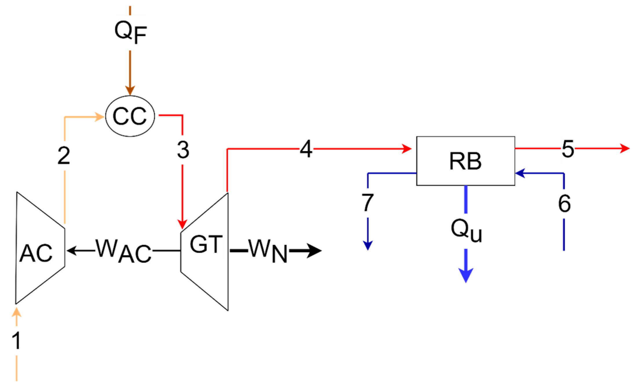
3. Case Study—Gas Turbine Cogeneration System

The cogeneration system with a simple gas turbine (Figure 1) is selected as an example to demonstrate how thermoeconomic modeling can effectively incorporate carbon credits. This system comprises four main components: an air compressor (AC), a combustion chamber (CC), a gas turbine (GT), and a recovery boiler (RB). The turbine generates power, part of which is utilized to drive the air compressor (WAC). The system produces two final products: net power (WN) and useful heat (QU). The fuel consumption is represented by (QF).
The main flow parameters of the physical structure, obtained through the Engineering Equation Solver—EES software [25], are presented in Table 1. Additionally, Table 2 provides the quantities of the primary productive flows. The reference conditions are specified as T 0 = 25 °C and P 0 = 1.0132 bar. Under these conditions, the mass flow of CO2 from the exhaust gases is m ˙ C O 2 = 2228 kg/h, considering natural gas as the fuel. Further details regarding this system can be found in [26]. The monetary unit cost of natural gas fuel is USD 24.04/MWh, which is based on the average value for the year 2022 in the international market [27].
In Table 3, the external monetary flows resulting from the cycle’s equipment are presented. These values were sourced from [26] and updated using the Chemical Engineering Cost Index (CEPCI) up until the year 2022 [28]. The cost of the carbon credit utilized in the analysis amounts to USD 85/ton, representing the average for the year 2022 as reported in [4].
Thermoeconomic modeling employs various types of diagrams: physical, productive, and comprehensive. While the physical diagram alone may not suffice to identify the waste cost formation process [26], the productive diagram is commonly utilized in most methodologies. One distinguishing aspect of functional methodologies like Thermoeconomic Functional Analysis (TFA) [23] and Engineering Functional Analysis (EFA) [8] is their ability to describe the cost formation process of thermal systems based on productive flows. This original feature has been adopted not only by TFA and EFA but also by other thermoeconomic methodologies, including the H&S Model [26] used in this paper.

3.1. Thermoeconomic Models

Thermoeconomic modeling employs the widely recognized E Model, which utilizes the total exergy flows to represent the physical and/or productive flows in diagrams. However, there are scenarios where it becomes necessary to decompose the exergy into its components. This is particularly important to isolate dissipative equipment and allocate waste costs accurately in thermal systems. An exergy disaggregation model known as the H&S Model [26] is available for this purpose in some cases. The H&S Model analyzes the behavior of thermodynamic cycles on the h–s plane, considering the variations in enthalpy and entropy of the working fluid, as proposed by [29]. This model allows for the separation of physical exergy into its enthalpic component (EH) and its entropic component (ES), as described in Equation (5).
The total exergy (E) can be mathematically defined by Equation (6) as the sum of the physical (EPH) and chemical (ECH) components. Notably, this definition excludes nuclear, magnetic, electrical, surface tension, kinetic, and potential effects [30].
E P H = E H E S
E = E H E S + E C H
The H&S Model introduces the concept of the environmental device (ENV) within the framework of the productive diagram, facilitating its interaction with other plant subsystems. This device assumes a critical role, in this methodology, in analyzing thermal systems, particularly in the context of waste cost allocation and internalization of environmental costs. Within ENV, both the physical component and the chemical component of the waste are dissipated with the device receiving air from the compressor inlet. The chemical component originates in the CC as a result of the combustion reaction, wherein the air and fuel mixture is transformed into combustion gases. It should be noted that the E Model does not include an explicit representation of the environment in the diagram. Nevertheless, this study also presents an approach for the integration and allocation of carbon credits into this methodology, in order to establish a comparison with the one that defines the environmental device with the same purpose and to demonstrate that it is also possible to adapt any thermoeconomic model for this objective.
Moreover, the environmental device (as employed in the H&S Model) assumes the responsibility of closing the cycle (Figure 2), thereby redistributing the costs associated with waste management across other plant components and, subsequently, to the final products.
Figure 2 illustrates the cogeneration cycle on the hs diagram, with the various processes denoted by numerical labels representing the respective components involved:
  • Process 1–2 corresponds to the compressor, with 1–2 s indicating isentropic compression.
  • Process 2–3 represents the combustion chamber.
  • Process 3–4 corresponds to the gas turbine, with 3–4 s denoting isentropic expansion.
  • Process 4–5 corresponds to the recovery boiler.
Upon reaching the exit of the recovery boiler (at point 5), the exhaust gases possess exergy, rendering them waste products. Despite the slight reduction in entropy of the working fluid caused by the recovery boiler (RB), the cycle remains incomplete. In contrast, a Rankine cycle is capable of achieving full closure through the condenser, wherein the entropy of the turbine’s output steam is reduced to that of saturated liquid at the pump inlet.
To complete the cycle in Figure 2, an environmental device (ENV) intervenes and facilitates process 5–1, effectively closing the loop. Within this device, flow 5 represents the exhaust gases, while flow 1 symbolizes the air drawn in by the compressor.

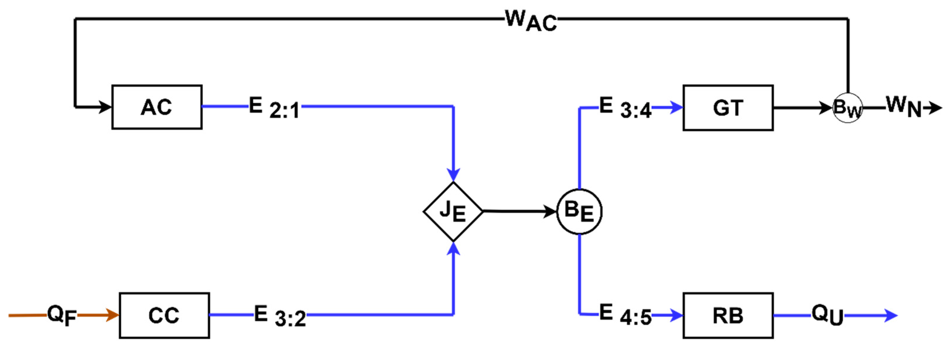
3.1.1. Productive Diagram

Figure 3 and Figure 4 illustrate the productive diagrams of the gas turbine cogeneration system as per the E and H&S Models, respectively. In the E Model, the depicted flows represent the changes in exergy between two physical states, denoted as i and j, following the expression given in Equation (7). Conversely, in the H&S Model, the productive flows on the diagrams represent the alterations in the enthalpic, entropic, and chemical components of exergy between states i and j, according to Equations (8)–(10), respectively.
E i : j = E i E j
E i : j H = E i H E j H
E i : j S = E i S E j S
E i : j C H = E i C H E j C H
In Figure 3 and Figure 4, the system components are depicted as real units or subsystems in the form of rectangles, while fictitious units called junctions (J) and bifurcations (B), represented by rhombuses and circles, respectively, are utilized to establish interconnections between these subsystems.
The characterization of fuel and product follows the SPECO approach [31] and is as follows: if the variation of specific exergy (or its components with a positive contribution to the exergy definition) exhibits a positive trend throughout the process; this variation, along with the exergy of energy flows generated within the component, determines the product. Conversely, if the variation of specific exergy (or its components with a positive contribution to the exergy) shows a negative trend throughout the process, this variation is combined with the exergy of energy flows supplied to the component in the input definition. The approach is reversed for components with a negative contribution to the exergy definition, such as the entropic component in the H&S Model. In this particular case, the H&S Model designates the entropic ( E 5 : 1 H ) and chemical ( E 3 : 2 C H ) components as inputs from the environment, while the entropic ( E 5 : 1 S ) component is identified as the product, as shown in Figure 4. On the other hand, E Model E (Figure 3) allocates the residue implicitly to the final products (WL and QU), proportionally to the exergetic inputs of the equipment generating the respective final products GT and RB.

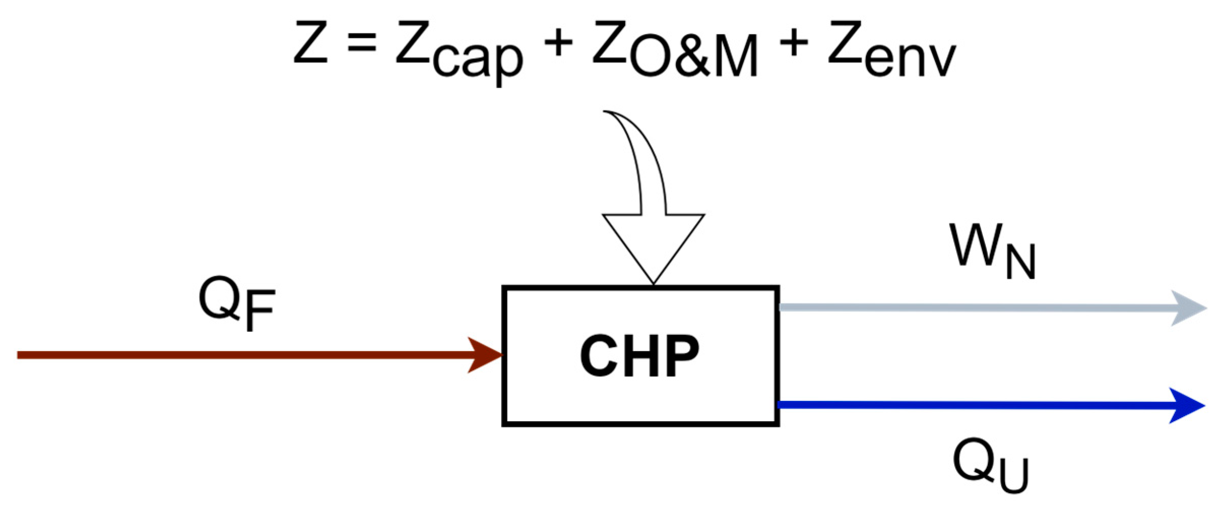
3.1.2. Monetary Cost Balance

Figure 5 presents the monetary cost balance for the H&S Model, represented in an expanded matrix format. This matrix is derived by applying the cost balance equation (Equation (1)) to each of the five subsystems (AC, CC, GT, RB, and ENV) as well as to the enthalpic (JH-BH) and entropic (JS-BS) junction–bifurcations within the productive diagram (Figure 4).
The internal valuation matrix comprises flows of exergy components, power, and useful heat, representing the entire process from the distribution of external resources to the determination of the final product costs. The cost matrix (or vector) constitutes the unknown factor in the modeling, incorporating the monetary unit cost of the flows generated within each subsystem. For instance, c A C denotes the monetary unit cost of the compressor (AC) product, which corresponds to the flow E 2 : 1 H .
Due to the application of the equality criterion, certain flows possess identical unit costs. Notable examples include E 3 : 2 H and E 3 : 2 C H ; E 4 : 5 S and Q U ; and W A C and W N . Moreover, all entropic component flows departing from JH-BH share the same unit cost, as do all entropic component flows leaving JS-BS.
The external valuation matrix encompasses the exergy of the fuel along with its corresponding unit cost, in addition to the external hourly cost of each subsystem resulting from capital and equipment operation and maintenance (Z). The junction–bifurcation components are considered dummy elements and, therefore, have a Z-cost of zero, as illustrated in the external valuation matrix depicted in Figure 5.
The Z term and the environmental representation device depicted in the diagrams play a crucial role in incorporating environmental costs within the field of thermoeconomics. Figure 6 provides a comprehensive overview of this device, illustrating its input and output flows, which contribute to the overall monetary cost equilibrium. The environmental device itself does not entail any costs associated with its acquisition, operation, or maintenance, as it serves as a symbolic representation of the atmospheric environment.
However, when an environmental treatment component (such as a filter, electrostatic precipitator, etc.) is introduced into the thermal system, which is not typically represented in the physical diagram, its cost can be internalized in the environmental device through the initial two terms on the right-hand side of Equation (4). Consequently, this cost is distributed across the entire system.
Furthermore, expenses related to fines, environmental licenses, permits, and carbon pricing values should also be internalized within the Z e n v factor. The exact treatment of carbon pricing values depends on whether they are considered revenue or expenses within the carbon market.
In the context of revenue generation, which can arise from a reduction in emissions below the specified level, resulting in the creation of tradable credits, a variable denoted as Z e n v assumes a negative value on the balance sheet. The environmental device responsible for closing the loop reallocates the associated costs to other equipment and final products within the plant. Consequently, this credit serves to diminish the overall monetary expenses and can exert an influence on the plant’s production decisions.
Conversely, expenses incurred in relation to carbon credits, such as the necessity to purchase credits due to the company’s failure to meet the stipulated emission reduction targets (or simply due to environmental consciousness and concerns regarding climate change), lead to a positive value for the Z e n v variable. This, in turn, results in an increase in the costs of other internal processes and final products within the plant.
To summarize, the equation depicted in Figure 6, referred to as Equation (11) in the text, plays a crucial role in understanding the aforementioned dynamics. An in-depth analysis of this equation can be conducted as follows:
  • The environmental device (ENV) does not have any hourly costs related to capital and operations and maintenance (O&M). However, if environmental treatment equipment, which is not typically part of the physical structure of the system, is used, these costs can be considered within Z E N V ;
  • The expenses for licenses and permits associated with the environment are accounted for in the Z e n v term;
  • Similarly, the costs related to the carbon market are also accounted for through the Z e n v term. When there is revenue, this term is represented as negative, and when there are expenditures, it is represented as positive.
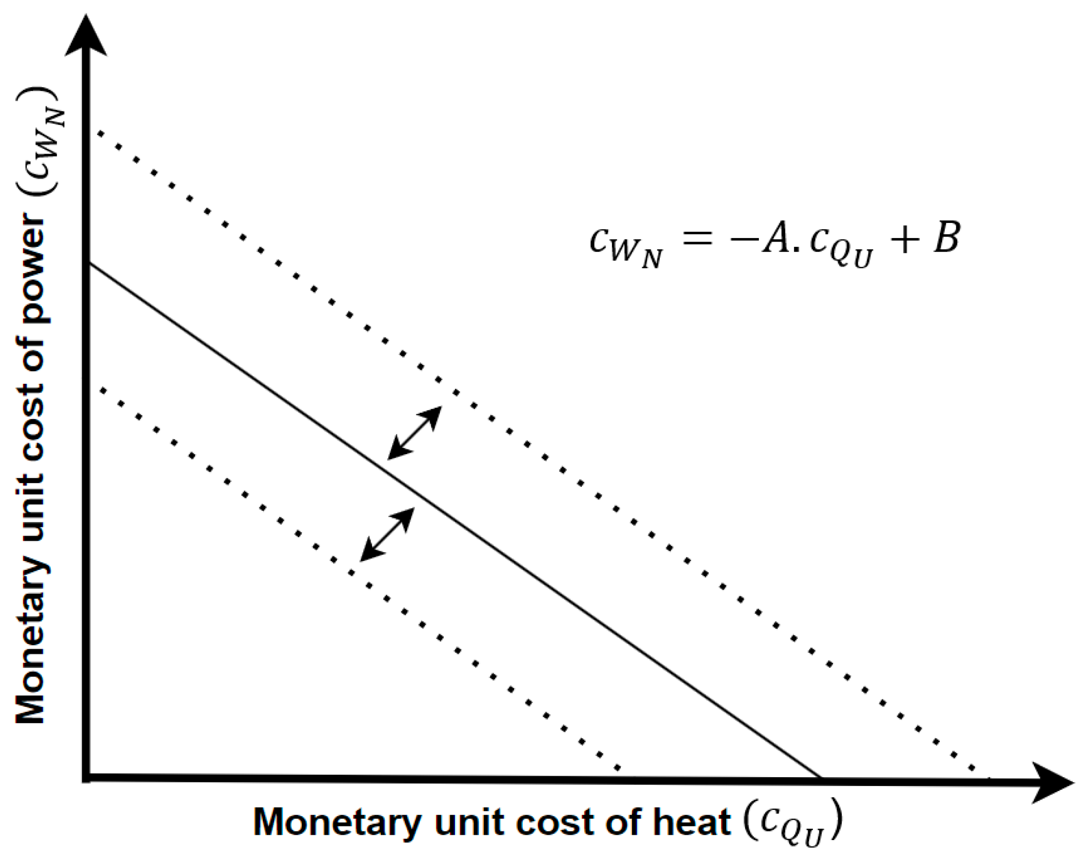
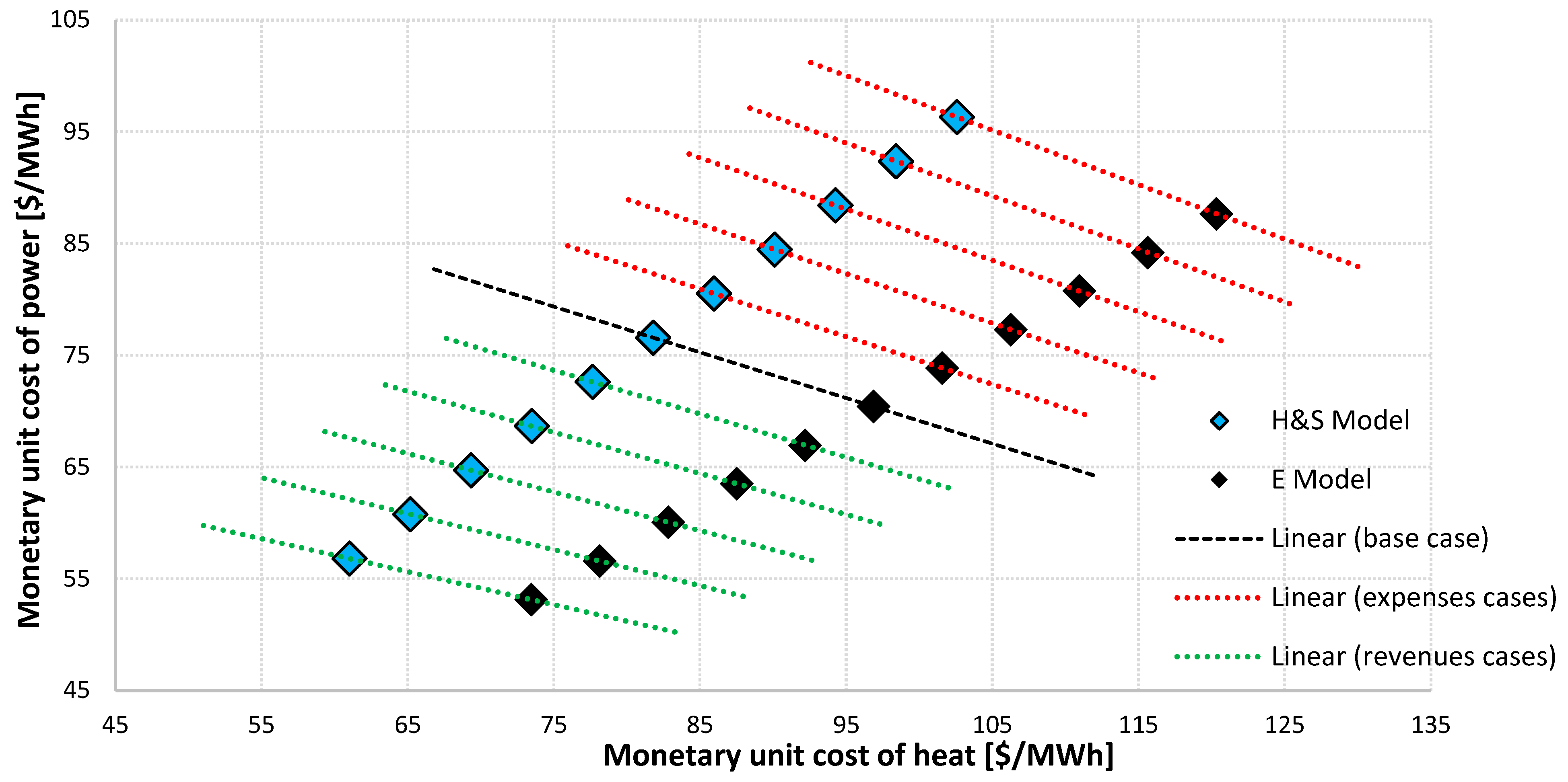
In all three cases, since the ENV device closes the loop (Figure 2), the costs are systematically distributed to the other subsystems and, consequently, to the final products of the plant, as shown in the case of the H&S Model (Figure 4).
Z E N V = Z c a p + Z O & M + Z e n v
In the case of thermoeconomic models that do not define the environment as an explicit device in the diagram, as is the case with Model E (Figure 3) in this paper, the internalization of carbon credits must be performed through the equipment generating emissions, the CC in such case. Conversely, when considering the cost of acquiring environmental control/treatment equipment, this model would need to depict such equipment in the physical and productive diagrams to facilitate appropriate cost allocation. However, these devices are dissipative, and several studies [32,33,34] have already demonstrated that Model E is not adequate for isolating them within the productive structure and thus analyzing them in a separate and appropriate manner.

3.1.3. Results

Figure 7 illustrates a generic cogeneration system, also known as a combined heat and power (CHP) system. This system generates two products, WN and QU, from a single fuel source, QF, similar to the gas turbine system depicted in Figure 1. By employing the cost balance equation (Equation (1)) to this generic cogeneration system, one obtains Equation (12), wherein c W N and c Q U represent the respective monetary unit costs of the final products, WN and QU. It is important to note that Equation (12) takes the form of a linear equation, y = A · x + B , and can be expressed in accordance with Equation (13).
c W N = Q U W N c Q U + c F · Q F + Z W N
c W N = A · c Q U + B
Irrespective of the applied thermoeconomic methodology, the solution to Equation (12) will consist of an ordered pair representing the monetary unit costs of the net power ( c W N ) and the useful heat ( c Q U ) . Several studies [16,35,36,37] have previously compared various methodologies for such problems and verified that these ordered pairs yield identical straight-line solutions when the system’s operational conditions are defined, including the net power-to-useful heat ratio and the global exergetic efficiency.
Figure 8 illustrates generic possibilities for this straight-line solution. In all cases, there is an inverse relationship between the unit cost of power and the unit cost of heat; that is, when the unit cost of power increases, the unit cost of heat decreases, and vice versa.
The central straight line, represented by the continuous line, denotes the specific condition for a cogeneration system. Changes in the thermodynamic model cause the straight line to shift to new positions parallel to the initial one [35,38], as depicted by the dashed lines in Figure 8.
Figure 9 illustrates the unit cost of the final products (represented as ordered pairs) in the cogeneration system under various scenarios. The cost values were determined using Equation (1) and applied to the diagrams in Figure 3 and Figure 4 for the E and H&S Models, respectively. In the case of the H&S Model, the cost balance is presented in matrix form in Figure 5, with a specific focus on Z E N V .
The data points situated along the central line in Figure 9 correspond to the base case, as mentioned in the figure’s caption. In this base case, carbon credit values are not taken into account or internalized.
It is noteworthy that an increase in emissions signifies a reduction in process efficiency, leading to higher production costs. Consequently, the solution line moves away from the origin, and the costs of the final products rise. Conversely, a reduction in emissions brings the solution line closer to the origin, indicating an improvement in process efficiency and a consequent decrease in the costs of the final products.
In order to conduct an analysis of the expenses and revenues within the carbon market, certain hypotheses were formulated and implemented. The initial scenario, referred to as the base case, considers that an increase in CO2 emissions leads to the system emitting beyond the established limit, necessitating the purchase of carbon credits and resulting in an expense for the plant. Another plausible real scenario that could lead to an escalation in costs involves a rise in the unit price of carbon credits owing to stricter emissions control regulations.
Conversely, in situations where emissions are reduced or removed, the system generates carbon credits that can be sold, thereby generating revenue. It is worth highlighting practical real scenarios capable of reducing and/or removing emissions in the industry. The utilization of mitigation equipment, such as carbon capture and storage systems (CCS), enables emission removal. In this case, the investment value (external cost per hour due to capital cost, operation, and maintenance of this equipment, Z) must be taken into account to assess and compare the cost of the investment with the potential revenue generated from carbon credits due to avoided emissions. Another feasible scenario for emission reduction involves substituting a more environmentally friendly fuel (e.g., natural gas with biogas or biomethane).
The H&S Model involves the internalization of the carbon credit value within the environmental device, represented as ( Z e n v > 0 ) for expenses and ( Z e n v < 0 ) for revenue. On the other hand, the E Model utilizes the internalization process through a combustion chamber (CC), with ( Z c a r b o n   c r e d i t > 0 ) for expenses and ( Z c a r b o n   c r e d i t < 0 ) for revenue.
To simulate the impact of these hypotheses, scenarios involving various percentages of emission increase (ranging from 10% to 50%) and reduction (ranging from −10% to −50%) concerning the base case were considered. The resulting Table 4 presents the unit costs of final products c Q U and c W N for each of these situations, along with the corresponding amount of carbon credits that would be generated and the associated costs (revenue and expense).
When conducting an analysis of c Q U and c W N , it has been observed that within the E Model, the costs of final products exhibit an approximate variation of 5% and 25% when there is a 10% and 50% increase or reduction in emissions, respectively, compared to the base case. Similarly, in the case of the H&S Model, these same scenarios lead to cost variations of approximately 5% and 26% for the final products. The observed cost fluctuations are attributed to the distinct criteria employed by each model, including the internalization of carbon credits in the CC and the environmental device.
Upon examining the carbon credits for the simulated scenarios, it has been noted that a 10% change in emissions results in the generation of 5.3 credits per day, equivalent to an expense or revenue of USD 455 per day. In the most extreme emission variation scenario (50%), the corresponding expenditure or revenue can reach USD 2273 per day. The utilization of the value derived from the purchase or sale of carbon credits can serve as a valuable indicator for companies in making decisions pertaining to the implementation of environmental equipment or the acquisition of carbon credits.
In all results, the ordered pair belongs to the straight solution, specific to the operating conditions of the plant. In addition, the models are consistent from a thermodynamic point of view according to the efficiencies and irreversibilities obtained.
Note that the primary objective of this study is to illustrate the application of the thermoeconomic methodology for integrating carbon pricing into cogeneration systems analysis. It is important to note that the study does not focus on analyzing the system’s behavior in terms of its capacity to increase or decrease emissions, nor does it involve defining the specific emission parameters that would govern the carbon market.
Examining the incorporation of environmental costs, such as carbon pricing, reveals an intriguing phenomenon denoted by Equation (12). This equation demonstrates that the Z term, and consequently Z e n v , influence the B coefficient of the linear equation (Equation (13)). Consequently, this adjustment leads to a parallel displacement of the initial straight line (base case) in comparison to the original condition. Specifically, when revenue is generated ( Z e n v < 0 ) through the sale of carbon credits, the straight line approaches the origin, resulting in a reduction in product costs. Conversely, for expenses ( Z e n v > 0 ) incurred in the purchase of carbon credits, the straight line shifts away from the origin, leading to an increase in production costs. It is essential to emphasize that the straight line transitions to distinct yet parallel positions. However, the slope remains unaltered due to the unchanged coefficient A.
Moreover, as the system conditions are defined and environmental costs are integrated, various thermoeconomic methodologies that account for the environmental aspect establish ordered pairs of power and heat costs lying on the same straight-line solution.

4. Conclusions

This research presents a comprehensive thermoeconomic approach to incorporate monetary environmental costs into multiproduct system assessments, demonstrated through a case study involving a gas turbine cogeneration system. The primary cost aspect addressed in this paper pertains to the valuation of carbon emissions. Nevertheless, the methodology also encompasses the internalization of other environmental expenses, including licensing, permits, and the procurement of environmental treatment and control equipment. Furthermore, the proposed methodology is adaptable for the allocation of both cost and emissions stemming from fuel utilization to final products across various categories of multiproduct systems, exemplified by industries such as sugarcane and alcohol, pulp and paper, and steel production.
In this study, two models, namely Models E and H&S, were employed for analysis. However, the primary focus is on H&S, as it offers a methodology that defines a crucial device responsible for representing the environment in the diagrams. This particular device plays a significant role in both the dissipation of cycle waste and the internalization of environmental costs, thereby enabling a systematic redistribution of costs across the system’s remaining components and final products. It is worth noting that any other thermoeconomic methodology, based on exergy and coherently defining this environmental device, could also be adopted by following similar methods. Moreover, models that do not explicitly define the ENV device in the diagram can internalize carbon credits within the equipment generating emissions. However, in the case of costs associated with the acquisition of environmental treatment/control equipment, these models might be limited in their analyses due to their inability to isolate this type of equipment (dissipative) within the productive structure.
The study presents the H&S Model as a viable instrument to achieve the objective by elucidating the inclusion of the carbon market and the internalization of carbon pricing and other environmental expenses in the analysis. In addition to explaining the calculation methodology, the study also examines the variations in monetary costs of cogeneration systems’ final products.
In conclusion, this research establishes that the proposed adapted methodology is consistent with the theoretical principles of thermodynamics and thermoeconomics. As a result, it can effectively facilitate the allocation of carbon credits to both the internal processes and final products of multiproduct systems.
By incorporating carbon credits into thermoeconomic modeling, it becomes possible: to evaluate the financial implications of carbon emissions and incentivize the reduction of greenhouse gases; to help in understanding the environmental impact of the thermal system; and to optimize the thermal system’s design and operation to maximize the economic benefits while minimizing emissions. It also can help in designing and implementing effective carbon pricing mechanisms and environmental policies to achieve emission reduction targets. Thus, companies and policymakers can gain a better understanding of the true costs and benefits of different thermal system configurations and make informed decisions that prioritize both economic and environmental sustainability.

Author Contributions

Conceptualization, P.R.d.F., I.C.B., R.G.d.S., M.A.B. and J.J.C.S.S.; methodology, P.R.d.F., I.C.B. and R.G.d.S.; software, I.C.B. and P.R.d.F.; validation, R.G.d.S. and J.J.C.S.S.; formal analysis, I.C.B., R.G.d.S. and M.A.B.; investigation, P.R.d.F., I.C.B. and R.G.d.S.; writing—original draft preparation, P.R.d.F. and R.G.d.S.; writing—review and editing, P.R.d.F., I.C.B., R.G.d.S., M.A.B. and J.J.C.S.S.; supervision, J.J.C.S.S.; project administration, J.J.C.S.S.; funding acquisition, J.J.C.S.S. All authors have read and agreed to the published version of the manuscript.

Funding

The APC was funded by “Fundação de Amparo a Pesquisa e Inovação do Espírito Santo—FAPES, T.O: 033/2024–P: 2024-J4KRS”.

Data Availability Statement

Data will be made available on request.

Acknowledgments

The authors would like to thank FAPES <Number T.O. 033/2024–P: 2024-J4KRS>, IFES, PPGEM-UFES, CNPq and CAPES.

Conflicts of Interest

The authors declare no conflict of interest.

Abbreviations

ACAir compressor
cMonetary unit cost (USD/MWh)
CCCombustion chamber
CCSCarbon capture and storage
CEPCIChemical Engineering Cost Index
CHPCombined heat and power
EExergy Flow (kW)
ENVEnvironmental device
GHGGreenhouse gas
GTGas turbine
IPCCIntergovernmental Panel on Climate Change
JBJunction–bifurcation
k * Exergetic unit cost (kW/kW)
QHeat (exergy) (kW)
RBRecovery boiler
WPower (kW)
YGeneric thermodynamic magnitude (kW)
ZHourly equipment cost (USD/h)
Greek symbols
λ Specific CO2 emission (g/MWh)
Subscripts and superscripts
0Reference conditions
CHChemical exergy (kW)
EnvEnvironmental
FFuel
HEnthalpic flow (kW)
i; jIndexes for productive components
inInlet
NNet
outOutlet
PHPhysical exergy (kW)
SEntropic flow (kW)
UUseful heat

References

  1. IPCC. Mitigation of Climate Change. 2022. Available online: https://report.ipcc.ch/ar6wg3/pdf/IPCC_AR6_WGIII_FinalDraft_FullReport.pdf (accessed on 9 May 2022).
  2. IEA. CO2 Emissions from Fuel Combustion: Overview-International Energy Agency; Paris. 2020. Available online: https://www.iea.org/reports/co2-emissions-from-fuel-combustion-overview (accessed on 28 April 2023).
  3. Instituto E+ Transição Energética. Manual de Termos e Conceitos: Transição Energética; Rio de Janeiro/RJ—Brasil. 2020. Available online: https://emaisenergia.org/publicacao/manual-de-termos-e-conceitos-transicao-energetica/ (accessed on 12 April 2023).
  4. SendeCO2. Available online: https://www.sendeco2.com/es/ (accessed on 18 March 2023).
  5. The World Bank. State and Trends of Carbon Pricing 2022; Washington, DC. 2022. Available online: https://openknowledge.worldbank.org/entities/publication/a1abead2-de91-5992-bb7a-73d8aaaf767f (accessed on 20 March 2023).
  6. IPCC. AR6 Synthesis Report Climate Change 2023. 2023. Available online: https://www.ipcc.ch/report/ar6/syr/ (accessed on 19 March 2023).
  7. Valero, A.; Serra, L.; Uche, J. Fundamentals of Exergy Cost Accounting and Thermoeconomics. Part I: Theory. J. Energy Resour. Technol. 2006, 128, 1–8. [Google Scholar] [CrossRef]
  8. von Spakovsky, M.R. Application of Engineering Functional Analysis to the Analysis and Optimization of the CGAM Problem. Energy 1994, 19, 343–364. [Google Scholar] [CrossRef]
  9. Dincer, İ.; Rosen, M.A. Exergy: Energy, Environment, and Sustainable Development, 1st ed.; Elsevier Science: Amsterdam, The Netherlands, 2007; ISBN 9780080445298. [Google Scholar]
  10. Palacios-Bereche, M.C.; Palacios-Bereche, R.; Ensinas, A.V.; Gallego, A.G.; Modesto, M.; Nebra, S.A. Brazilian Sugar Cane Industry—A Survey on Future Improvements in the Process Energy Management. Energy 2022, 259, 124903. [Google Scholar] [CrossRef]
  11. Man, Y.; Yan, Y.; Wang, X.; Ren, J.; Xiong, Q.; He, Z. Overestimated Carbon Emission of the Pulp and Paper Industry in China. Energy 2023, 273, 127279. [Google Scholar] [CrossRef]
  12. Mishra, R.; Singh, R.K.; Gunasekaran, A. Adoption of Industry 4.0 Technologies for Decarbonisation in the Steel Industry: Self-Assessment Framework with Case Illustration. Ann. Oper Res. 2023. [Google Scholar] [CrossRef]
  13. Faria, P.R.; dos Santos, R.G.; Santos, J.J.; Barone, M.A.; Miotto, B.M. On the Allocation of Residues Cost Using Conventional and Comprehensive Thermoeconomic Diagrams. Int. J. Thermodyn. 2021, 24, 134–149. [Google Scholar] [CrossRef]
  14. Barone, M.A.; dos Santos, R.G.; Faria, P.R.; Lorenzoni, R.A.; Lourenço, A.B.; Santos, J.J.C.S. On the Arbitrariness and Complexity in Thermoeconomics Due to Waste Cost and Supplementary Firing Treatment. Eng. Sci. 2022, 17, 328–342. [Google Scholar] [CrossRef]
  15. Faria, P.R.; dos Santos, R.G.; Santos, J.J.C.S.; Barone, M.A.; Miotto, B.M.F. On the Allocation of Residues Cost in Thermoeconomics Using a Comprehensive Diagram. In Proceedings of the ECOS 2020—The 33rd International Conference on Efficiency, Cost, Optimization, Simulation and Environmental Impact of Energy Systems, Osaka, Japan, 29 June–3 July 2020; pp. 2444–2456. [Google Scholar]
  16. Cerqueira, S.A.A.G.; Nebra, S.A. Cost Attribution Methodologies in Cogeneration Systems. Energy Convers. Manag. 1999, 40, 1587–1597. [Google Scholar] [CrossRef]
  17. Modesto, M.; Nebra, S.A. Analysis of a Repowering Proposal to the Power Generation System of a Steel Mill Plant through the Exergetic Cost Method. Energy 2006, 31, 3261–3277. [Google Scholar] [CrossRef]
  18. Santos, R.G.; Faria, P.R.; Santos, J.J.C.S.; da Silva, J.A.M. Thermoeconomic Modeling for CO2 Allocation in Steam and Gas Turbine Cogeneration Systems. In Proceedings of the ECOS 2015—The 28th International Conference on Efficiency, Cost, Optimization, Simulation and Environmental Impact of Energy Systems, Pau, France, 29 June–3 July 2015. [Google Scholar]
  19. Faria, P.R.; Barone, M.A.; Santos, R.G.; Santos, J.J.C.S. The Environment as a Thermoeconomic Diagram Device for the Systematic and Automatic Waste and Environmental Cost Internalization in Thermal Systems. Renew. Sustain. Energy Rev. 2023, 171, 113011. [Google Scholar] [CrossRef]
  20. Faria, P.R.; Torres, C.; Santos, J.J.; Valero, A. On the Thermoeconomic Modelling of Thermal Waste Cost Allocation and Diagnosis of Malfunctions for Environmental Aspects Assessment. In Proceedings of the ECOS 2022—The 35th International Conference on Efficiency, Cost, Optimization, Simulation and Environmental Impact of Energy Systems, Copenhagen, Denmark, 3–7 July 2022. [Google Scholar]
  21. Fortes, A.F.C.; Carvalho, M.; da Silva, J.A.M. Environmental Impact and Cost Allocations for a Dual Product Heat Pump. Energy Convers. Manag. 2018, 173, 763–772. [Google Scholar] [CrossRef]
  22. Lozano, M.A.; Valero, A.; Serra, L.M. Theory of Exergetic Cost and Thermoeconomic Optimization. In Energy Systems and Ecology, Proceedings of the ENSEC’ 93: Energy Systems and Ecology: Proceedings of the International Conference: Cracow, Poland, 5–9 July 1993; Szargut, J., Kolenda, Z., Tsatsaronis, G., Ziebik, A., Eds.; University of Zaragoza: Zaragoza, Spain; Volume 1, pp. 339–350.
  23. Frangopoulos, C.A. Application of the Thermoeconomic Functional Approach to the CGAM Problem. Energy 1994, 19, 323–342. [Google Scholar] [CrossRef]
  24. Torres, C.; Valero, A.; Rangel, V.; Zaleta, A. On the Cost Formation Process of the Residues. Energy 2008, 33, 144–152. [Google Scholar] [CrossRef]
  25. F-Chart Software Engineering Equation Solver—EES 2017. Available online: http://www.fchart.com (accessed on 17 August 2022).
  26. Santos, J.J.C.S. Aplicação Da Neguentropia Na Modelagem Termoeconômica de Sistemas. Ph.D. Dissertation, Federal University of Itajubá, Itajubá, Brazil, 2009. (In Portuguese). [Google Scholar]
  27. Trading Economics. Available online: https://pt.tradingeconomics.com/commodity/natural-gas (accessed on 19 March 2023).
  28. Chemical Engineering CEPCI. Available online: https://www.chemengonline.com/category/business-economics/ (accessed on 19 March 2023).
  29. Valero, A.; Royo, J.; Lozano, M.A. The Characteristic Equation and Second Law Efficiency of Thermal Energy Systems. In Proceedings of the International Conference Second Law Analysis of Energy Systems: Towards the 21st Century, Rome, Italy, 5–7 July 1995; Sciubba, E., Moran, M.J., Eds.; La Sapienza: Rome, Italy, 1995; pp. 99–112. [Google Scholar]
  30. de Oliveira Junior, S. Exergy: Production, Cost and Renewability; Green Energy and Technology; Springer: London, UK, 2013; ISBN 978-1-4471-4164-8. [Google Scholar]
  31. Lazzaretto, A.; Tsatsaronis, G. SPECO: A Systematic and General Methodology for Calculating Efficiencies and Costs in Thermal Systems. Energy 2006, 31, 1257–1289. [Google Scholar] [CrossRef]
  32. Santos, R.G.; Faria, P.R.; Barone, M.A.; Lorenzoni, R.A.; Orozco, D.J.R.; Santos, J.J. On the Thermoeconomic Diagnosis through the Localized Physical Exergy Disaggregation for Dissipative Component Isolation. In Proceedings of the ECOS 2021—The 34th International Conference on Efficiency, Cost, Optimization, Simulation and Environmental Impact of Energy Systems, Taormina, Italy, 27 June–2 July 2021; Volume 1, pp. 450–461. [Google Scholar]
  33. dos Santos, R.G.; Lourenço, A.B.; Faria, P.R.; Barone, M.A.; Santos, J.J.C.S. A New Exergy Disaggregation Approach for Complexity Reduction and Dissipative Equipment Isolation in Thermoeconomics. Entropy 2022, 24, 1672. [Google Scholar] [CrossRef] [PubMed]
  34. Abreu, R.P.; Correia, V.H.L.; Lourenço, A.B.; Marques, A.d.S.; Carvalho, M. Thermoeconomic and Thermoenvironmental Analysis of the Chilled Water System in a Shopping Mall. Int. J. Refrig. 2022, 134, 304–311. [Google Scholar] [CrossRef]
  35. Santos, R.G.; Faria, P.R.; Santos, J.J.C.S.; Da Silva, J.A.M.; Donatelli, J.L.M. The Effect of the Thermodynamic Models on the Thermoeconomic Results for Cost Allocation in a Gas Turbine Cogeneration System. Rev. Eng. Térmica 2015, 14, 47. [Google Scholar] [CrossRef]
  36. Santos, R.G.; Lourenço, A.; Faria, P.R.; Barone, M.A.; Santos, J.J. A Comparative Study of a New Exergy Disaggregation Approach with Conventional Thermoeconomic Methodologies for Cost Allocation in an Organic Rankine Cycle Powered Vapor Compression Refrigeration System. In Proceedings of the ECOS 2022—The 35th International Conference on Efficiency, Cost, Optimization, Simulation and Environmental Impact of Energy Systems, Copenhagen, Denmark, 3–7 July 2022; pp. 1057–1068. [Google Scholar]
  37. Bhering Trindade, A.; Luiza Grillo Renó, M.; José Rúa Orozco, D.; Martín Martinez Reyes, A.; Aparecido Vitoriano Julio, A.; Carlos Escobar Palacio, J. Comparative Analysis of Different Cost Allocation Methodologies in LCA for Cogeneration Systems. Energy Convers. Manag. 2021, 241, 114230. [Google Scholar] [CrossRef]
  38. de Araújo, L.R.; Morawski, A.P.; Barone, M.A.; Donatelli, J.L.M.; Santos, J.J.C.S. On the Effects of Thermodynamic Assumptions and Thermoeconomic Approaches for Optimization and Cost Allocation in a Gas Turbine Cogeneration System. J. Braz. Soc. Mech. Sci. Eng. 2020, 42, 323–341. [Google Scholar] [CrossRef]
Figure 1. The physical structure: cogeneration system.
Processes 12 00705 g001
Figure 2. The environment device in open cycles.
Processes 12 00705 g002
Figure 3. Productive diagram—E Model.
Processes 12 00705 g003
Figure 4. Productive diagram—H&S Model.
Processes 12 00705 g004
Figure 5. Monetary cost balance in matrix form.
Processes 12 00705 g005
Figure 6. Cost balance in the environmental device.
Processes 12 00705 g006
Figure 7. Accounting flows in cogeneration.
Processes 12 00705 g007
Figure 8. Unit cost solution line.
Processes 12 00705 g008
Figure 9. Monetary unit cost variation due to emissions.
Processes 12 00705 g009
Table 1. Main physical flow parameters of the system.
Physical Flow m ˙ (kg/s)T (°C)P (bar)
No.Description
1Air14.7225.001.0132
2Air14.72230.205.1040
3Gases14.94850.004.8480
4Gases14.94537.301.0207
5Gases14.94151.101.0132
6Water2.48760.0020.400
7Steam2.487212.420.000
Table 2. Productive flows (exergetic basis).
EquipmentFlowQuantity (kW)
Air compressor (AC)WAC3113.03
Combustion chamber (CC)QF11,630.96
Gas turbine (GT)WGT5546.50
WN2433.47
Recovery boiler (RB)QU2246.32
Table 3. Equipment external monetary cost.
EquipmentZ (USD/h)
Air compressor (AC)25.33
Combustion chamber (CC)9.04
Gas turbine (GT)34.37
Recovery boiler (RB)21.71
Table 4. Monetary unit cost [USD/MWh] and carbon credit for the simulated situations.
EmissionsE ModelH&S ModelCarbon Credit/DayUSD/Day
( c Q U ) ( c W N ) ( c Q U ) ( c W N )
+50%120.3387.66102.5796.3226.7−2273
+40%115.6484.2198.4192.3721.4−1818
+30%110.9580.7694.2688.4216.0−1364
+20%106.2677.3190.1084.4710.7−909
+10%101.5773.8685.9580.525.3−455
Base case96.8870.4181.7976.5700
−10%92.1966.9677.6472.625.3455
−20%87.5163.5173.4868.6710.7909
−30%82.8260.0669.3364.7216.01364
−40%78.1456.665.1760.7721.41818
−50%73.4553.1561.0256.8226.72273
Disclaimer/Publisher’s Note: The statements, opinions and data contained in all publications are solely those of the individual author(s) and contributor(s) and not of MDPI and/or the editor(s). MDPI and/or the editor(s) disclaim responsibility for any injury to people or property resulting from any ideas, methods, instructions or products referred to in the content.

