Bi-Level Inverse Robust Optimization Dispatch of Wind Power and Pumped Storage Hydropower Complementary Systems

Abstract

This paper presents a bi-level inverse robust economic dispatch optimization model consisting of wind turbines and pumped storage hydropower (PSH). The inner level model aims to minimize the total generation cost, while the outer level introduces the optimal inverse robust index (OIRI) for wind power output based on the ideal perturbation constraints of the objective function. The OIRI represents the maximum distance by which decision variables in the non-dominated frontier can be perturbed. Compared to traditional methods for quantifying the worst-case sensitivity region using polygons and ellipses, the OIRI can more accurately quantify parameter uncertainty. We integrate the grid multi-objective bacterial colony chemotaxis algorithm and the bisection method to solve the proposed model. The former is adopted to solve the inner level problem, while the latter is used to calculate the OIRI. The proposed approach establishes the relationship between the maximum forecast deviation and the minimum generation cost associated with each non-dominated solution in the optimal load allocation. To demonstrate its economic viability and effectiveness, we simulate the proposed approach using real power system operation data and conduct a comparative analysis.

1. Introduction

The global power industry has placed significant emphasis on net zero emission, proposed during the 21st UN Climate Change Conference. The future is poised for a substantial surge in the utilization of renewable energy for power generation. Nevertheless, the inherent unpredictability of renewable resources poses a challenge, leading to potential imbalances between supply and demand. To mitigate the impact of renewable energy generators on the power system, the paramount focus is on advancing energy storage systems. Pumped storage hydropower (PSH) has gained widespread popularity due to its substantial capacity and cost-effectiveness [1]. Javed et al. [2] discussed the economic, environmental, and technical aspects of solar–wind–PHS systems, affirming the positive role of PHS in integrating renewable energy into the power systems. The integration of PSH has increased the flexibility and efficiency of renewable power generation.

With the large-scale integration of wind power into the grids, the impact of wind power’s uncertainty on the scheduling and control operations of the power system has become increasingly pronounced [3]. Therefore, it is crucial to address the uncertainties associated with wind power when studying the coordinated scheduling of wind power–PSH systems. Many researchers have explored the relationship between uncertainty and wind power distribution using probabilistic models, including interval prediction [4], quantile regression prediction [5], the scenario generation method [6], two-stage stochastic programming [7], chance-constrained programming [8], and interval forecasting [9]. Interval prediction, quantile regression prediction, and the scenario generation method primarily focus on characterizing uncertain variables. However, these methods face challenges, such as high computational complexity and the inability to guarantee computational accuracy and security, limiting their further development. The last three methods rely on deterministic probability distribution models and require significant sampling computations. However, due to the impact of wind power uncertainty [10], these optimal dispatch models are complex, high-dimensional, non-convex, and non-differentiable multi-objective optimization problems. As a result, traditional methods often yield inaccurate density functions for wind power output, limiting their practical application.

Robust optimization methods are widely used because they do not require specific probability distributions to deal with wind power uncertainty. Since the 1970s, Soyster et al. [11] pioneered the use of linear robust optimization methods for solving uncertain linear programming problems. To overcome the limitations of this approach, a constraint protecting the nominal parameter level was introduced in the literature [12]. A maximum perturbation is added to the left side of the constraint equation, and an optimization dualization technique is used to integrate the equations, resulting in a linear robust model. Jin et al. [13] provide a more comprehensive definition of robustness in optimization problems. Robustness refers to the ability of the non-dominated solution set to maintain certain performance characteristics when decision variables are perturbed. It is often used to characterize the sensitivity of parameters to disturbances.

References [14,15] tackle supply and demand uncertainties by constructing a stochastic robust optimization model. The Benders’ decomposition method is then employed to solve this model. However, the solutions obtained through this method may fall outside of the specified range during parameter perturbations. References [16,17] introduce a bi-level interval robust scheduling optimization model that accounts for the unpredictable nature of wind power. This model is utilized to formulate wind power scheduling plans for the next few hours. By applying strong duality theory, the model is transformed into a quadratic programming problem for the solution. However, interval robust optimization methods tend to search for overly conservative solutions that meet the fluctuation constraints in the objective functions. Ji et al. [18] improve upon conventional fuzzy scheduling optimization problems by incorporating fuzzy numbers to account for the inherent uncertainty in wind power ramping time. The methodology generates an uncertain set that encompasses worst-case scenarios, presenting a scheduling model based on fuzzy robust optimization methods. This multi-objective robust design based on fuzzy theory commonly employs the weighted analysis method for formulating objective functions, introducing a notably subjective element into the methodology. Gunawan et al. [19] propose a multi-objective robust optimization method by introducing the concept of the worst-case sensitivity region (WCSR). The WCSR’s radius acts as a robust indicator and is included in the constraints, transforming the problem into a constrained multi-objective optimization. However, this method has some limitations, such as the subjective construction of uncertainty and the lack of capability to search for a globally optimal solution. To overcome these issues, we propose a bi-level inverse robust optimization dispatch model for wind power–PSH complementary systems. The main contributions of this paper are summarized as follows.

Firstly, this paper presents a novel approach for improving the integration of wind power into the electricity grid while achieving economic efficiency. The proposed approach is based on the characteristics of pumped storage hydropower stations and develops a bi-level inverse robust economic dispatch optimization model that considers the uncertainties of wind power and the participation of pumped storage hydropower stations in scheduling. Secondly, the proposed model incorporates ideal disturbance constraints on the objective function, which are based on decision makers’ preferences. We use hypersphere contraction and expansion to explore decision variable points with the best robustness in the non-dominated solution set. The OIRI is introduced to represent the maximum distance at which decision variables in the non-dominated frontiers can be perturbed. It provides the worst-case perturbation for each point in each dimension of the high-dimensional space, which enhances the generating units’ robustness against disturbances and establishes the optimal relationship between wind power integration and the objective function. Thirdly, we propose a novel approach combining the grid multi-objective bacterial colony chemotaxis algorithm with the bisection method. The inner level problem is addressed by the grid multi-objective bacterial colony chemotaxis algorithm, and the OIRI is calculated using the bisection method. The effectiveness of the proposed model and algorithm is validated through simulations using actual grid-connected data. This approach can be useful for dispatchers in optimizing the schedule of wind power–PSH complementary systems.

2. Inverse Robust Optimization Preliminaries

This subsection briefly introduces the general bi-level inverse robust optimization model. Inner level optimization aims to obtain superior decision vectors and feasible solutions within the feasible domain. The outer level seeks to derive the maximum range of robustness among the results obtained from the inner layer by imposing ideal disturbance constraints. According to the conventional robust optimization model and the worst-case sensitivity region, we have the following bi-level inverse robust model.

Outer level problem:

$$find\left\{OIRI\left(\mathit{x}\right)=\max {‖\mathit{x}-{\mathit{x}}_0‖}_2,\mathit{f}\right\}$$

(1)

$$s.t. \mathit{f}\left({\mathit{x}}_0\right)\in \overline{U\left(\mathit{f}\left(\mathit{x}\right),\mathit{d}\right)}\cap \mathsf{\Phi }$$

(2)

$$\mathit{d}=\mathit{f}\left(\mathit{x}\right)-\mathit{f}\left({\mathit{x}}_0\right), u\left(\mathit{f}\right)=\left\{\mathit{d}\left|\mathit{d}\in U\left(0,\mathit{\epsilon }\right)\right.\right\}, \mathit{d}\in u\left(\mathit{f}\right)$$

(3)

Inner level problem:

$$\mathrm{Minimize} \mathit{f}={\left[f_1,f_2,\cdots ,f_m\right]}^T$$

(4)

$$g_j\left(\mathit{x}\right),\underset{d\in u\left(\mathit{f}\right)}{\max }{g}_j\left({\mathit{x}}_0\right)\le 0,j=1,2,\dots ,J$$

(5)

$$h_k\left(\mathit{x}\right),\underset{d\in u\left(\mathit{f}\right)}{\max }{h}_k\left({\mathit{x}}_0\right)=0,k=1,2,\dots ,K$$

(6)

where $\mathit{x}={\left[x_1,x_2,\dots ,x_n\right]}^T$ is the n-dimensional decision vector and ${\mathit{x}}_0$ is the decision vector satisfying all constraints in the inner and outer levels. The optimal inverse robust indicator OIRI will be defined in Definition 1. f is the m-dimensional objective function vector; d denotes the ideal disturbance vector; $\mathit{\epsilon }={\left[{\epsilon }_1,{\epsilon }_2,\dots ,{\epsilon }_m\right]}^T$ is the m-dimensional vector consisting of ideal disturbance coefficients; and all elements are positive. U(0,$\mathit{\epsilon }$) represents the neighborhood of the zero point composed of all points with a distance less than $\epsilon$ from the circle; $\overline{U\left(·\right)}$ is the closure of the neighborhood of $U(·)$; $\mathsf{\Phi }$ denotes the inner decision vector space; $g_j(\mathit{x})$/$h_k(\mathit{x})$ represent inequality/equality constraints, respectively; J and K are the number of inequality constraints and equality constraints, respectively; and m and n are the number of objective functions and decision variables, respectively.

The Pareto front of this model (1)–(6) is referred to as the inverse robust Pareto frontier. The following definitions are given:

Definition 1.

Assuming $\Omega$ is the feasible region of the inner level problem, for any $\mathit{x}\in \Omega$ and any given ideal disturbance coefficients $\mathit{\epsilon }>0$, there exists a convex neighborhood of ${∆}_{max}\subset \Omega$ so that for any ${\mathit{x}}_0\in {∆}_{max}$, $\mathit{y}=\mathit{f}\left({\mathit{x}}_0\right)$ satisfies the inner and outer constraints. ${∆}_{max}$ is referred to as the optimal inverse robust indicator (OIRI) if and only if the following two conditions are met:

(1)

The mapping function $\mathit{f}$ satisfies $\mathit{f}:{∆}_{max}⟼U(\mathit{f}\left(\mathit{x}\right),\epsilon )\bigcap \mathsf{\Phi }$.

(2)

There is no region $\Lambda$ that satisfies both $\mathsf{\Lambda }\subset \mathsf{\Omega }$ and ${∆}_{max}\subseteq \mathsf{\Lambda }$, so that $\mathit{f}:\mathsf{\Lambda }⟼\overline{U(\mathit{f}\left(\mathit{x}\right),\epsilon )}\bigcap \mathsf{\Phi }$.

Equation (2) indicates that when solving the outer level problem, it is necessary to ensure that the objective function values of boundary points fall within the feasible domain and the range of ideal disturbance constraints. The optimal inverse robust indicator represents the maximum distance by which a decision vector $\mathit{x}$, satisfying Equations (2)–(4) in the non-dominated frontier, can be perturbed outward.

3. Bi-Level Inverse Robust Model for Wind Power–PSH Complementary Systems

The scheduling model developed in this section is a bi-level inverse robust optimization model that takes into account thermal power plants, pumped storage hydropower stations, and wind power. The model is structured as Equations (1)–(6) and considers the decision makers’ expected deviation range from the total generation cost and forecast results as ideal disturbance constraints. Additionally, the model defines the OIRI as the maximum wind power fluctuation that the optimization results can tolerate. The inner level of the model minimizes the total generation cost, while the outer level solves for the OIRI and the corresponding total generation cost $\mathit{f}$, thus determining the Pareto frontier.

The objective function of the outer level problem is defined as

$$\mathrm{OIRI}=\max {\displaystyle \sum _{t=1}^T{‖{\mathit{P}}_t^w-{\mathit{P}}_t^{w_0}‖}_2}$$

(7)

where ${\mathit{P}}_t^w={\left[P_{j,t}^w\right]}_{N_w\times 1}$ is the non-dominated decision vector of wind power obtained from the inner level problem and ${\mathit{P}}_t^{w_0}={\left[P_{j,t}^{w_0}\right]}_{N_w\times 1}$ is the decision vector within $U({\mathit{P}}_t^w,\mathit{\epsilon })$. A larger OIRI indicates greater robustness in the inner level optimization results for ${\mathit{P}}_t^w$, implying a stronger ability of the wind power generation plan to withstand fluctuations.

The total generation cost $f$ is defined as

$$f={\displaystyle \sum _{t=1}^T\left({\displaystyle \sum _{i=1}^{N_c}{C}_{i,t}\left(P_{i,t}\right)}+{\displaystyle \sum _{j=1}^{N_w}{\phi }_j{\left(\left(P_{j,t}^w or P_{j,t}^{w_0}\right)-P_{j,t}^{prw}\right)}^2}+{\displaystyle \sum _{k=1}^{N_p}\left[S{C}_{k,t}\left(h_{k,t}\right)+{\varphi }_k{\left(P_{k,t}^{ps}-P_{k,t}^{prps}\right)}^2\right]}\right)}$$

(8)

where T is the number of dispatch time intervals. $N_c/N_w/N_p$ represent the number of thermal units, wind farms, and PSHs, respectively. $P_{j,t}^w/P_{j,t}^{\mathit{prw}}$ denote the output power/forecasted output power of wind farm j in the inner level at period t, respectively; $P_{j,t}^{w_0}$ represents the output power of wind farm j in the outer level at period t; $P_{j,t}^{\mathit{ps}}/P_{j,t}^{\mathit{prps}}$ denote the output power/forecasted output power of PSH j in the inner level at period t, respectively; and the fuel cost $C_{i,t}\left(P_{i,t}\right)$ of the thermal unit i can be expressed as a quadratic function in relation to its output power $P_{i,t}$. ${\phi }_j\left(\left(P_{j,t}^w or P_{j,t}^{w_0}\right),P_{j,t}^{\mathit{prw}}\right)$ denotes the penalty cost of wind farm j deviating from the planned output at period t. ${\phi }_j/{\varphi }_k$ are the penalty coefficients. ${\mathit{SC}}_{k,t}\left(P_{j,t}^{\mathit{ps}}\right)$ is the sum of start-up and shut-down costs. It can be expressed as

$$S{C}_{k,t}\left(h_{k,t}\right)=h_{k,t}\left(1-h_{k,t-1}\right)S_k^{ps}+h_{k,t-1}\left(1-h_{k,t}\right)D_k^{ps}$$

(9)

where $h_{k,t}$ denotes the PSH’s working state, taking 1 for start and taking 0 for stop and $S_{k,t}^{\mathit{ps}}/D_{k,t}^{\mathit{ps}}$ are the start-up cost and shut-down cost of the PSH k.

As shown in (5) and (6), the constraints of the inner level are listed as follows.

(1)

Power balance constraints:

$${\displaystyle \sum _{i=1}^{N_c}{P}_{i,t}}+{\displaystyle \sum _{j=1}^{N_w}{P}_{j,t}^w}+{\displaystyle \sum _{k=1}^{N_p}{P}_{k,t}^{ps}}=D_t$$

(10)

where $D_t$ is the total power load.

(2)

Generation limit constraints:

$${\underset{\_}{P}}_i\le P_i\le {\overline{P}}_i$$

(11)

$${\underset{\_}{P}}_j^w\le P_j^w\le {\overline{P}}_j^w$$

(12)

where ${\underset{\_}{P}}_i/{\overline{P}}_i$ are the lower/upper limits of thermal unit i, respectively. ${\underset{\_}{P}}_j^w/{\overline{P}}_j^w$ are the lower/upper output limits of wind farm j, respectively.

(3)

Climbing constraints for thermal units:

$$-r{p}_{i,t}^d\cdot \Delta T\le P_{i,t}-P_{i,t-1}\le r{p}_{i,t}^u\cdot \Delta T$$

(13)

where ${\mathit{rp}}_{i,t}^d/{\mathit{rp}}_{i,t}^u$ are the maximum upward/downward ramping rates, respectively. $∆T$ is the dispatch time interval.

(4)

Spinning reserve constraints:

$$\left\{\begin{array}{l}{\displaystyle \sum _{i=1}^{N_c}{h}_{i,t}\left({\overline{P}}_{i,t}^{spin}-P_{i,t}\right)}+{\displaystyle \sum _{k=1}^{N_k}{P}_{k,t}^{ps}}\ge S{P}_t^{up}\\ {\overline{P}}_{i,t}^{spin}=h_{i,t-1}\cdot \min \left(h_{i,t-1}{\overline{P}}_{i,t},P_{i,t-1}+r{p}_{i,t}^u\cdot \Delta T\right)\\ S{P}_t^{up}={\beta }^c{\displaystyle \sum _{i=1}^{N_c}{P}_{i,t}}+{\beta }^w{\displaystyle \sum _{j=1}^{N_w}{P}_{j,t}^w}\end{array}\right.$$

(14)

$$\left\{\begin{array}{l}{\displaystyle \sum _{i=1}^{N_c}{h}_{i,t}\left(P_{i,t}-{\underset{¯}{P}}_{i,t}^{spin}\right)}+{\displaystyle \sum _{k=1}^{N_k}{\underset{¯}{P}}_{k,t}^{ps}}\ge S{P}_t^{dn}\\ {\underset{¯}{P}}_{i,t}^{spin}=h_{i,t-1}\cdot \max \left(h_{i,t-1}{\underset{¯}{P}}_{i,t},P_{i,t-1}-r{p}_{i,t}^d\cdot \Delta T\right)\\ S{P}_t^{dn}={\beta }^w{\displaystyle \sum _{j=1}^{N_w}{P}_{j,t}^w}\end{array}\right.$$

(15)

where $h_{i,t}$ is the binary variable and denotes the working state of thermal unit i at period t; ${\underset{\_}{P}}_{i,t}^{\mathit{spin}}/{\overline{P}}_{i,t}^{\mathit{spin}}$ are the minimum/maximum feasible outputs of thermal unit i at period t; and ${\mathit{SP}}_t^{\mathit{up}}/{\mathit{SP}}_t^{\mathit{dn}}$ are the upward/downward requirements of power systems at period t. ${\beta }^c/{\beta }^w$ are the spinning reserve rates of the thermal unit and the wind farm.

(5)

Transmission constraints:

$${\underset{¯}{TP}}_l\le {\displaystyle \sum _{i=1}^{N_c}T{F}_{l,i}{P}_{i,t}}+{\displaystyle \sum _{j=1}^{N_w}T{F}_{l,j}{P}_{j,t}^w}+{\displaystyle \sum _{k=1}^{N_p}T{F}_{l,k}{P}_{k,t}^{ps}}\le {\overline{TP}}_l$$

(16)

where ${\underset{\_}{\mathit{TP}}}_l/{\overline{\mathit{TP}}}_l$ are the lower/upper power flow limits of line l and ${TF}_{l,i}$ denotes the power transfer distribution factors from unit i to line l.

(6)

Minimum on and off time constraints:

$$\left\{\begin{array}{l}\left(T_{i,t-1}^{on}-Z_i^{on}\right)\left(h_{i,t-1}-h_{i,t}\right)\ge 0\\ \left(T_{i,t-1}^{off}-Z_i^{off}\right)\left(h_{i,t}-h_{i,t-1}\right)\ge 0\end{array}\right.$$

(17)

where $T_{i,t-1}^{\mathit{on}}/T_{i,t-1}^{\mathit{off}}$ are the start-up/shut-down times of thermal unit i at period t − 1, respectively and $M_i^{\mathit{on}}/M_i^{\mathit{off}}$ represent the minimum start-up/shut-down times of the thermal power unit i.

(7)

PSH’s capacity constraints:

In actual operation, PSHs are required to satisfy constraints regarding reservoir water balance. We adopt a daily energy balance mode wherein the electricity consumed during pumping and the electricity generated during generation are equal throughout the day, thus ensuring that the reservoir water level remains relatively unchanged at the beginning and end of the day.

$$-{\eta }_k{\displaystyle \sum _{t=1}^T{\displaystyle \sum _{k=1}^{N_p}{P}_{k,t}^{ps}}}={\displaystyle \sum _{t=1}^T{\displaystyle \sum _{k=1}^{N_p}{P}_{k,t}^{ps}}}$$

(18)

where ${\eta }_k$ is the energy conversion efficiency of PSH k.

(8)

Start–stop frequency constraints:

$${\displaystyle \sum _{t=1}^T\left|h_{k,t}-h_{k,t-1}\right|}\le {\overline{TH}}_k$$

(19)

where ${\overline{TH}}_k$ is the maximum daily start–stop times of PSH k. Frequent starts and stops can accelerate the deterioration of the generator, leading to increased maintenance requirements, higher repair costs, and a potentially shorter operational lifespan. Equation (19) refers to limitations imposed on how frequently the PSH can be start up or shut down within a given period. When the PSH k starts up or shuts down, $\left|h_{k,t}-h_{k,t-1}\right|$ is equal to 1. Summing up $\left|h_{k,t}-h_{k,t-1}\right|$ over an operating cycle T yields the total number of start-ups and shut-downs of PSH k.

(9)

Ideal perturbation constraint:

$${‖\mathit{f}\left({\mathit{P}}_t^w\right)-\mathit{f}\left({\mathit{P}}_t^{w_0}\right)‖}_2\le \epsilon$$

(20)

Equation (20) ensures that the outer level optimization satisfies the ideal disturbance constraints. In this section, we present a dispatch model that utilizes bi-level inverse robust optimization theory. This model provides the optimal load allocations for conventional thermal power units, wind farms, and PSHs. Additionally, it will identify the maximum insensitivity regions relative to each optimal allocation point when there are uncertain parameters in the system undergoing perturbations.

4. Solution Procedure

The model developed in this paper has an inherent coupling between the inner and outer layers. Therefore, a singular intelligent optimization algorithm is not enough for obtaining effective solutions. To address the inner level optimization problem, the grid multi-objective bacterial colony chemotaxis algorithm is employed.

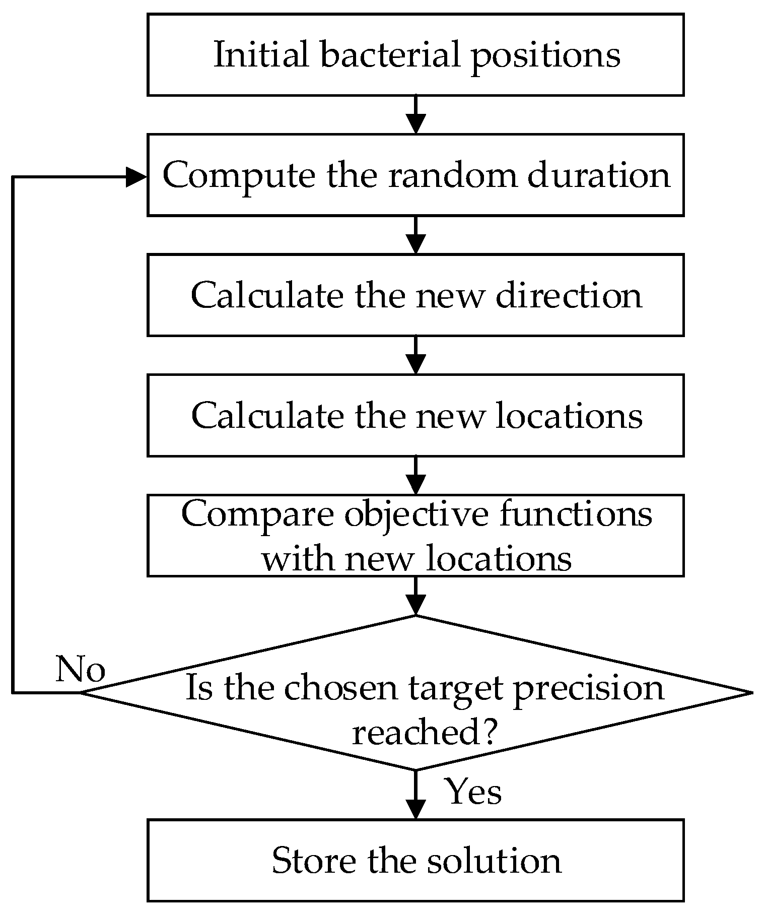
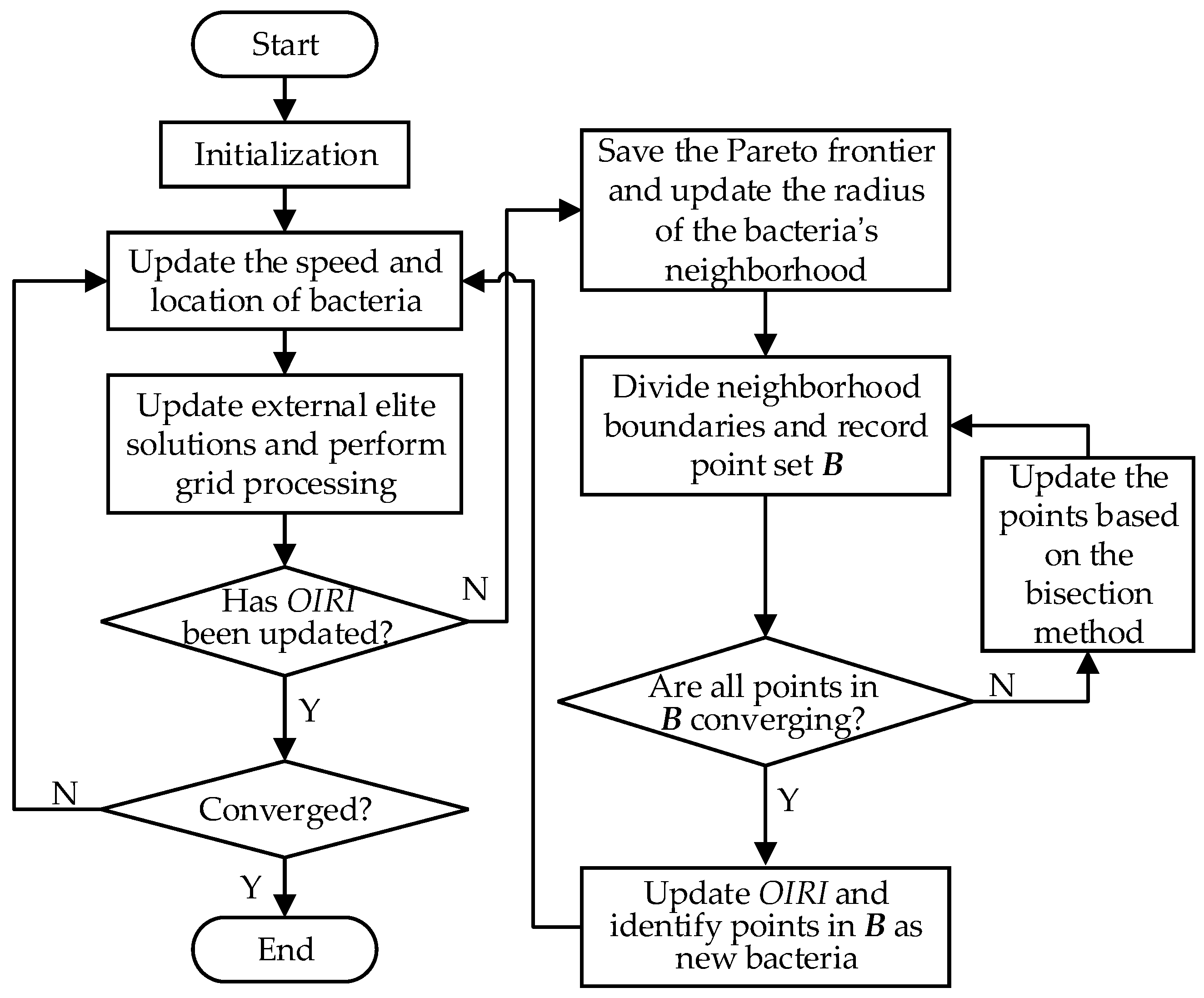
4.1. Brief Introduction of the Multi-Objective Bacterial Colony Chemotaxis Algorithm

The role of the multi-objective bacterial colony chemotaxis algorithm [20,21] is to solve the inner level optimization problem. The trajectory of a bacterium comprises consecutive linear paths interspersed with instantaneous changes in direction, with each path defined by its speed, direction, and duration. All paths are characterized by a uniform, constant speed. Upon changing direction, a bacterium selects a new trajectory based on a probability distribution that exhibits azimuthal symmetry relative to the preceding direction. The angle between consecutive trajectories follows a probability distribution, while the duration of each trajectory is determined by an exponentially declining probability distribution. Notably, both the angle and duration probability distributions are unaffected by the parameters of the preceding trajectory.

Here, x is used to represent decision variables $P_{i,t}$ and $P_{j,t}^{\mathit{ps}}$. Before applying the multi-objective bacterial colony chemotaxis algorithm, all constraints are added as penalty terms to the objective function. Figure 1 shows the flow chart of the multi-objective bacterial colony chemotaxis algorithm, which can be briefly explained as follows.

Step 1: Initialize bacterial positions. Generate $N_{ba}$ bacteria randomly in this model. The velocity v is assumed to be a scalar constant value.

Step 2: Compute the random duration $\tau$ that follows an exponential probability density function:

$$P\left(X=\tau \right)=\frac{1}{\gamma }{e}^{-\tau /\gamma }$$

(21)

$$\gamma =\left\{\begin{array}{l}{\gamma }_0 \mathrm{if} {\mathit{x}}_{pre}\succ {\mathit{x}}_{cur}\\ {\gamma }_0\left(1+b\ast \min \left|\frac{f_{mpr}}{l_{pr}}\right|\right) \mathrm{if} {\mathit{x}}_{pre}\prec {\mathit{x}}_{cur}\end{array}\right.$$

(22)

$${\gamma }_0={\xi }^{0.03}\cdot {10}^{-1.73}\hspace{1em}b={\gamma }_0\cdot \left({\gamma }_0^{-1.54}\cdot {10}^{0.6}\right)$$

(23)

where ${\gamma }_0$ and b are the minimal mean time and dimensionless parameter, respectively. They can be calculated through (23) according to reference [21]. $\xi$ is the calculation precision. $f_{ipr},i=\mathrm{1,2},\dots ,m$ is the difference between the actual and the previous function values. $l_{pr}$ is the vector connecting the previous and the actual positions in the parameter space. ${\mathit{x}}_{pre}$ and ${\mathit{x}}_{\mathrm{cur}}$ are the previous and current locations of bacteria.

The position and motion of bacteria is defined by a radius $r_0$ and n − 1 angles $\mathit{\theta }=\left\{{\theta }_1,{\theta }_2,\dots ,{\theta }_{n-1}\right\}$.

$$x_1=r_0{\displaystyle {\prod }_{s=1}^{n-1}\cos \left({\theta }_s\right)} , x_i=r_0\sin \left({\theta }_{i-1}\right){\displaystyle {\prod }_{s=1}^{n-1}\cos \left({\theta }_s\right),i=2,3,\dots ,n}$$

(24)

Step 3: Calculate the new direction. The angle ${\theta }_i$ between the previous and new directions follows a Gaussian distribution, governing both left and right turns, respectively.

$$P\left(X_i={\theta }_i,v_i={\mu }_i\right)=\frac{1}{{\sigma }_i\sqrt{2\pi }}\exp {\left[-\frac{\left({\theta }_i-v_i\right)}{2{\sigma }_i^2}\right]}^2$$

(25)

$$P\left(X_i={\theta }_i,v_i=-{\mu }_i\right)=\frac{1}{{\sigma }_i\sqrt{2\pi }}\exp {\left[-\frac{\left({\theta }_i-v_i\right)}{2{\sigma }_i^2}\right]}^2$$

(26)

where ${\theta }_i\in \left[0,{180}^{\circ }\right]$. The expectation value ${\mu }_i$, variance ${\sigma }_i$, and correlation time ${\tau }_C$ are determined by the formulation:

$${\mu }_i={62}^{\circ }\left(1-\exp \left(-{\tau }_C{\tau }_{pr}\right)\right) {\sigma }_i={26}^{\circ }\left(1-\exp \left(-{\tau }_C{\tau }_{pr}\right)\right)$$

(27)

where ${\tau }_{pr}$ is the duration of the previous step.

Step 4: Calculate the new locations ${\mathit{x}}_{\mathrm{new}1}$ and ${\mathit{x}}_{\mathrm{new}2}$. The new locations are calculated through the following equations:

$${\mathit{x}}_{\mathrm{new}1}={\mathit{x}}_{\mathrm{pre}}+v\cdot \tau$$

(28)

$${\mathit{x}}_{\mathrm{new}2}={\mathit{x}}_{\mathrm{pre}}-2\times \mathrm{U}\left(0,1\right)\times \left({\mathit{x}}_{\mathrm{pre}}-{\mathit{x}}_{\mathrm{cen}}\right)$$

(29)

$${\mathit{x}}_{\mathrm{cen}}=\frac{1}{N_{ba}}{\displaystyle \sum _{i=1}^{N_{ba}}{x}_i}$$

(30)

where $\mathrm{U}\left(0,1\right)$ is a random number governed by the uniform distribution.

Step 5: Determine the new location ${\mathit{x}}_{\mathrm{new}}$. By comparing ${\mathit{x}}_{\mathrm{new}1}$ with ${\mathit{x}}_{\mathrm{new}2}$, all bacteria choose the better one as their new locations. Terminate iteration when the change in the objective function value is less than the target precision $\xi$; otherwise, proceed to Step 2.

4.2. Solution Method for the Bi-Level Inverse Robust Model

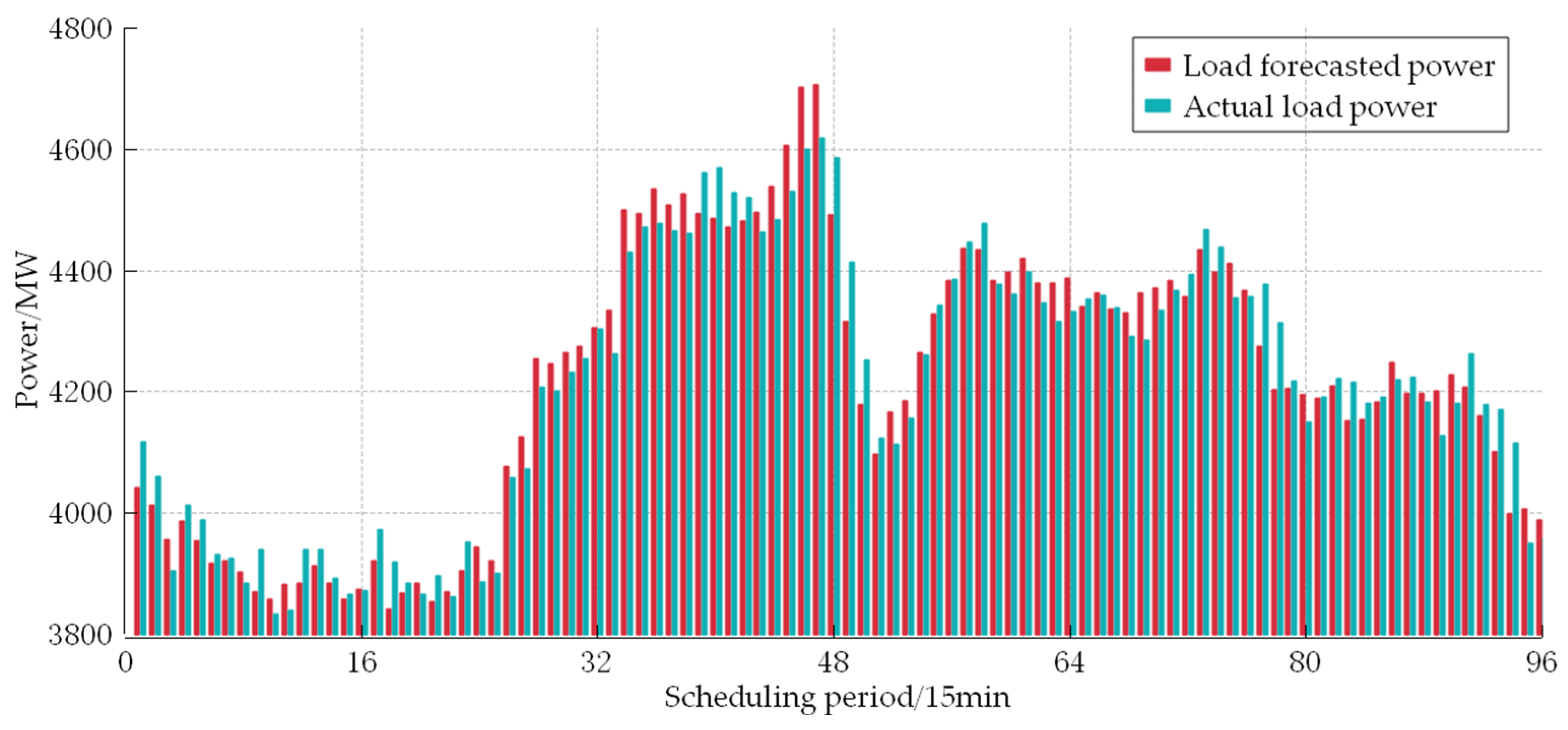
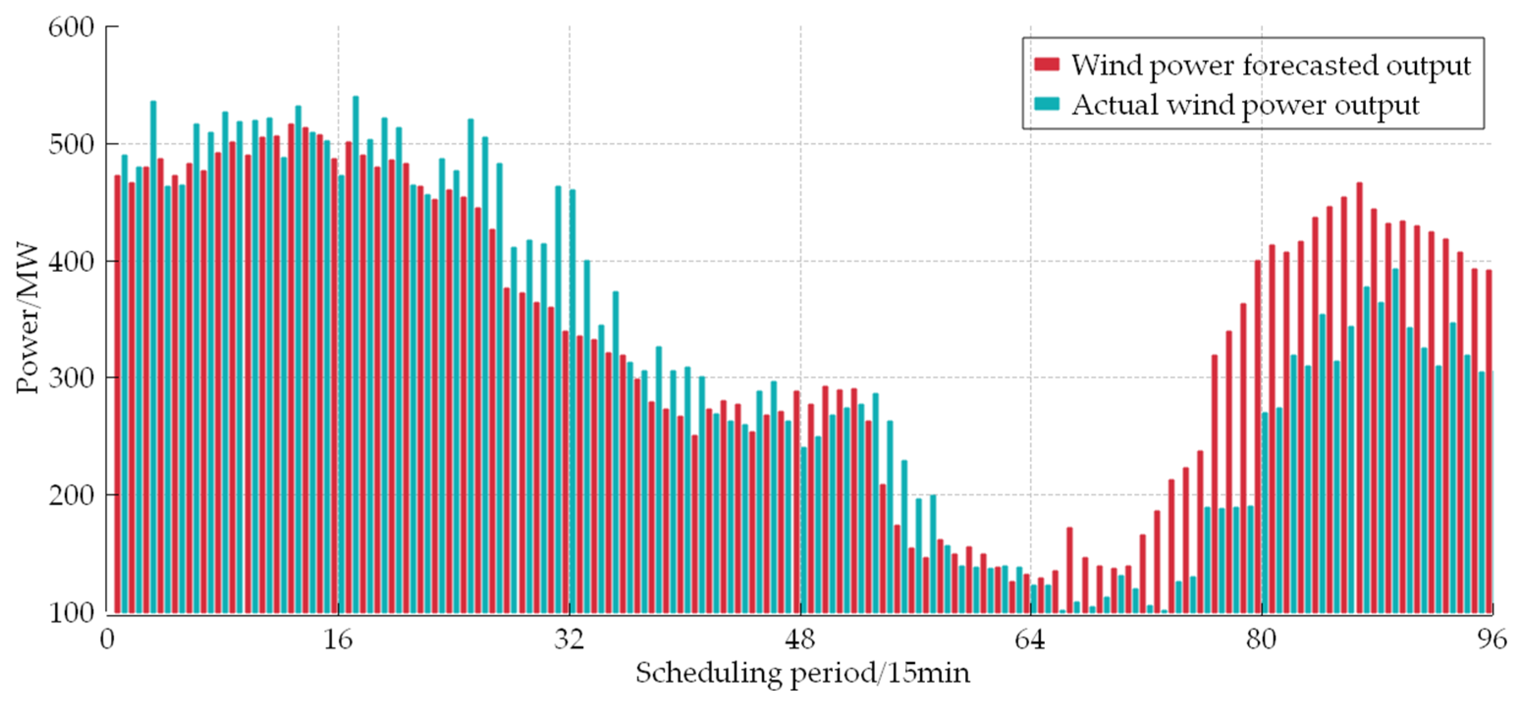
To calculate the OIRI for the outer level optimization problem, the hypersphere can be used to quantify maximum uncertainty. This involves partitioning the hyperspherical surface to facilitate the outward expansion of each small arc face. This results in a more accurate irregular super-enclosed surface characterized by the radial distance r and polar angle $\theta =\left[{\theta }_1,{\theta }_2,\dots ,{\theta }_{n-1}\right]$. Its maximum radius corresponds to the OIRI. Applying the boundary principle, we replace the discussion of changes across the entire domain with an examination of variations in domain boundary points.

Let x be equivalent to ${\mathit{P}}_t^w$. Assume x is a non-dominated solution obtained from the inner level problem. Consider a spherical neighborhood, denoted as O(x), around $\mathit{x}=\left[x_1,x_2,\dots ,x_n\right]$, with a radius denoted as $r_0$. Every point on the boundary of O(x), denoted as $\partial O\left(\mathit{x}\right)$, can be expressed using parametric equations. Let ${\mathit{x}}_0=\left[x_{01},x_{02},\dots ,x_{0n}\right]$ and ${\mathit{x}}_0\in \partial O\left(\mathit{x}\right)$, so we have

$$\left\{\begin{array}{l}{x}_{01}=x_1+r_0\cos {\theta }_1\\ x_{02}=x_2+r_0\sin {\theta }_1\cos {\theta }_2\\ \cdots \\ x_{0n}=x_n+r_0\sin {\theta }_1\sin {\theta }_2\cdots \cos {\theta }_{n-1}\end{array}\right.$$

(31)

where ${\theta }_1,{\theta }_2,\dots ,{\theta }_{n-2}\in \left[0,\pi \right]$, ${\theta }_{n-1}\in \left[\mathrm{0,2}\pi \right]$. We adopt a uniform sampling method to sample points on the boundary $\partial O\left(\mathit{x}\right)$. The boundary $\partial O\left(\mathit{x}\right)$ is divided into M parts, where $M={\lambda }_1·{\lambda }_2,\dots ,{\lambda }_{n-1}$ $\left({\lambda }_i\in N^{+},i=1,2,\dots ,n-1\right)$. Define a set $\mathit{B}=\left\{{\mathit{x}}_0={\mathit{x}}_{q_1{q}_2\dots q_{n-1}}|1\le q_i\le {\lambda }_i,q_i\in N^{+},i=1,2,..,n-1\right\}$, so we have

$${\mathit{x}}_{q_1{q}_2\dots q_{n-1}}={\left[\begin{array}{l}{x}_1+r_0\cos \left(\frac{\pi }{{\lambda }_{n-1}}{\eta }_1\right),\\ x_2+r_0\sin \left(\frac{\pi }{{\lambda }_{n-1}}{\eta }_1\right)\cos \left(\frac{\pi }{{\lambda }_{n-2}}{\eta }_2\right),\dots ,\\ x_n+r_0\sin \left(\frac{\pi }{{\lambda }_{n-1}}{\eta }_1\right)\dots \cos \left(\frac{\pi }{{\lambda }_2}{\eta }_{n-2}\right)\cos \left(\frac{2\pi }{{\lambda }_1}{\eta }_{n-1}\right)\end{array}\right]}^T$$

(32)

After defining

$$D\left(\mathit{x}\right)={\left[{‖f_1\left(\mathit{x}\right)-f_1\left({\mathit{x}}_0\right)‖}_2,{‖f_2\left(\mathit{x}\right)-f_2\left({\mathit{x}}_0\right)‖}_2,\dots ,{‖f_m\left(\mathit{x}\right)-f_m\left({\mathit{x}}_0\right)‖}_2\right]}^T$$

(33)

the bisection method can be applied to approximate a larger hyperregion, ensuring that when decision variables are perturbed within this region, the function values are constrained within a certain range. In other words, adjusting each point ${\mathit{x}}_0\in \mathit{B}$ ensures that ${\mathit{x}}_0$ satisfies ${‖D\left({\mathit{x}}_0\right)‖}_{\infty }\in \left[\epsilon -{\delta }_{\epsilon },\epsilon +{\delta }_{\epsilon }\right]$, and ${\delta }_{\epsilon }$ is a predefined convergence accuracy. The specific steps of the bisection method are as follows.

Step 1: Initializing set $\mathit{B}$.

(1) If there is a point ${\mathit{x}}_0\in \mathit{B}$ that satisfies ${‖D\left({\mathit{x}}_0\right)‖}_{\infty }\in \left[\epsilon -{\delta }_{\epsilon },\epsilon +{\delta }_{\epsilon }\right]$, then the values of $\mathit{f}\left({\mathit{x}}_0\right)$ and $〈r_0,\theta 〉$ are stored, and the process proceeds to Step 2.

(2) If there are two points ${\mathit{x}}_1,{\mathit{x}}_2\in \mathit{B}$ and ${\mathit{x}}_1\ne {\mathit{x}}_2$ that satisfy ${‖D\left({\mathit{x}}_1\right)‖}_{\infty }<\epsilon -{\delta }_{\epsilon }$ and ${‖D\left({\mathit{x}}_2\right)‖}_{\infty }>\epsilon +{\delta }_{\epsilon }$, the process proceeds to Step 2. Otherwise, adjust the radial radius through the bisection method.

(3) If for any ${\mathit{x}}_0\in \mathit{B}$ that satisfies ${‖D\left({\mathit{x}}_1\right)‖}_{\infty }>\epsilon -{\delta }_{\epsilon }$, then $r_1=2r_0$ and $r_2=r_0+0.5\left(r_1-r_0\right)$. If for any ${\mathit{x}}_0\in \mathit{B}$ that satisfies ${‖D\left({\mathit{x}}_2\right)‖}_{\infty }<\epsilon +{\delta }_{\epsilon }$, then $r_1=0.5r_0$ and $r_2=r_0+0.5\left(r_1-r_0\right)$. Calculate the size of ${‖D\left({\mathit{x}}_0\right)‖}_{\infty }$ in the set $\mathit{B}$ based on radial radius $r_1$ and $r_2$.

Step 2: Update the points in set $\mathit{B}$.

Define ${\mathit{B}}_1=\left\{{\mathit{x}}_0|{‖D\left({\mathit{x}}_0\right)‖}_{\infty }<\epsilon -{\delta }_{\epsilon } \mathrm{or} {‖D\left({\mathit{x}}_0\right)‖}_{\infty }>\epsilon +{\delta }_{\epsilon }\right\}$. As in the procedure in Step 1, scale the radial radius of all ${\mathit{x}}_0\in {\mathit{B}}_1$ until ${‖D\left({\mathit{x}}_0\right)‖}_{\infty }\in \left[\epsilon -{\delta }_{\epsilon },\epsilon +{\delta }_{\epsilon }\right]$ is satisfied. Record the angular and radial information of ${\mathit{x}}_0$.

Step 3: Calculate $O\mathrm{I}\mathrm{R}\mathrm{I}={max}_{{\mathit{x}}_0\in \mathit{B}}{r}_0$ and all angles and radial directions $〈r_0,\theta 〉$.

In traditional multi-objective optimization models, points within the decision space often exhibit better robustness, whereas feasible solutions near the boundaries of the decision space tend to have poorer robustness. When non-dominated solutions are located on or near the boundary, the perturbation of objective function values cannot extend beyond the super-neighborhood, and the corresponding perturbation of decision space vectors cannot expand outward. Here, an adaptive reduction of perturbation space is employed, limiting the range of perturbations of decision vectors within the feasible domain. This approach avoids redundant evaluations and reduces computational burden.

We integrate the grid multi-objective bacterial colony chemotaxis algorithm and the bisection method to solve the proposed model. Figure 2 illustrates the calculation process.

Step 1: System parameter initialization. It involves setting parameters, such as calculation precision, bacteria migration rate, initial positions of the bacterial colony, ideal error constraints, error precision, and the number of boundary samples, among others.

Step 2: Update the speed and location of bacteria. According to the conventional bacterial colony chemotaxis algorithm [20,21], a bacterium will make a decision by comparing ${\mathit{x}}_{\mathrm{new}1}$ with ${\mathit{x}}_{\mathrm{new}2}$ and choose the better one as its new location ${\mathit{x}}_{\mathrm{new}}$.

Step 3: Update the external Pareto set and perform grid processing. Guide the mutation of bacteria using non-dominance-based variation. Select non-dominated solutions from the new generation population and incorporate them into the Pareto set while simultaneously removing inferior solutions from the Pareto set.

Step 4: If the OIRI has been updated, proceed to Step 5. Otherwise, go to Step 6.

Step 5: Terminate the program if the convergence accuracy or the maximum number of iterations is reached. Otherwise, go back to Step 2.

Step 6: Save the Pareto frontier and update the radius of the bacteria’s neighborhood.

Step 7: Divide neighborhood boundaries and record point set $\mathit{B}$.

Step 8: If all points in set $\mathit{B}$ have converged, go to Step 9. Otherwise, go to Step 6.

Step 9: Update the OIRI and identify points in $\mathit{B}$ as new bacteria. Define the crowd distance of ${\mathit{x}}_{\mathrm{new}1}/{\mathit{x}}_{\mathrm{new}2}$ as ${\mathit{CD}}_1/{\mathit{CD}}_2$.

The OIRI and f have been defined by (7) and (8). The new location can be calculated as follows:

(1) If two out of the three conditions $\mathit{f}\left({\mathit{x}}_{\mathrm{new}1}\right)\prec \mathit{f}\left({\mathit{x}}_{\mathrm{new}2}\right)$, $\mathrm{OIRI}\left({\mathit{x}}_{\mathrm{new}1}\right)>\mathrm{OIRI}\left({\mathit{x}}_{\mathrm{new}2}\right)$, and ${\mathit{CD}}_1>{\mathit{CD}}_2$ are satisfied, then let ${\mathit{x}}_{\mathrm{new}}={\mathit{x}}_{\mathrm{new}1}$;

(2) If two out of the three conditions $\mathit{f}\left({\mathit{x}}_{\mathrm{new}1}\right)\succ \mathit{f}\left({\mathit{x}}_{\mathrm{new}2}\right)$, $\mathrm{OIRI}\left({\mathit{x}}_{\mathrm{new}1}\right)<\mathrm{OIRI}\left({\mathit{x}}_{\mathrm{new}2}\right)$, and ${\mathit{CD}}_1<{\mathit{CD}}_2$ are satisfied, then let ${\mathit{x}}_{\mathrm{new}}={\mathit{x}}_{\mathrm{new}2}$;

(3) Otherwise, maintain the original position unchanged, ${\mathit{x}}_{\mathrm{new}}=\mathit{x}$.

Go to Step 2.

5. Case Study

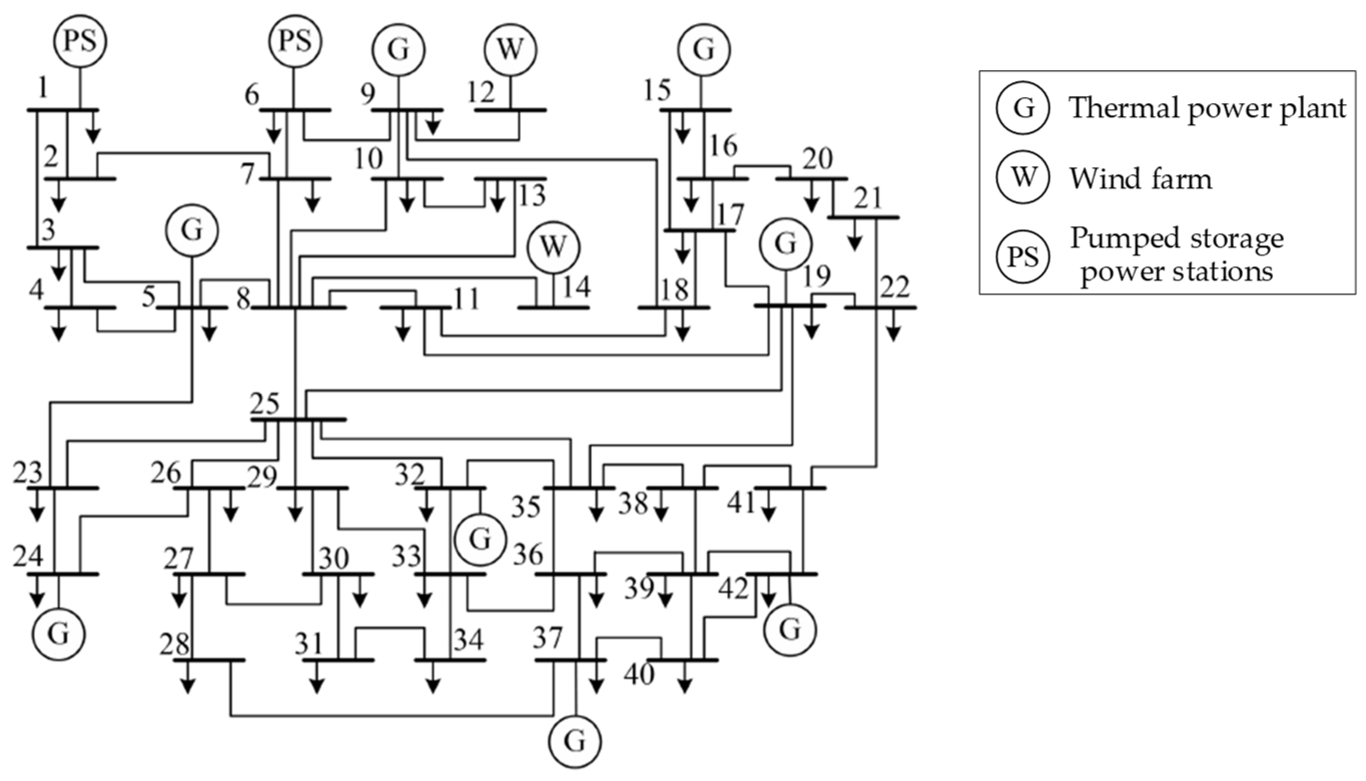
5.1. Modified 42-Bus Power System

In the modified 42-bus power system, the participating generating units include eight thermal power plants consisting of twenty-two units with capacities of 540 MW (four units), 315 MW (five units), 300 MW (five units), 270 MW (three units), and 180 MW (five units), with a total installed capacity of 6945 MW. There are two wind farms with a total capacity of 1080 MW, and the system wind power penetration rate ranges from approximately 12% to 20%. There are also two pumped storage power stations, each with a capacity of 270 MW. The maximum and minimum reservoir capacities are 2.0015 × 10⁶ m³ and 4.8388 × 10⁵ m³, respectively. The network topology is illustrated in Figure 3. The numbers in the Figure 3 represent the bus numbers.

The ramping rates for thermal power units are 5% of their rated capacity. The start-up and shut-down cost for each PSH is USD 585. The penalty factor for deviation from the planned output for PSHs is 0.5. The fuel cost $C_{i,t}\left(P_{i,t}\right)$ of the thermal unit i can be expressed as a quadratic function, and its cost coefficients for thermal power units are provided in

Table 1. Cost coefficient of thermal power units.

Rated Power/MW	Pmax/MW	Pmin/MW	ai	bi	ci
540	540	270	0.00037	18.315	807.11
315	315	157.5	0.00051	17.435	843.80
297	297	148.5	0.00053	19.241	710.68
270	270	135	0.00063	22.789	521.00
180	180	90	0.00066	22.181	634.71

.

In Table 1, the units for a_i, b_i, and c_i are USD/MW²h, USD/MWh, and USD/h, respectively. Based on the pre-scheduled plan, one PSH will pump water at its rated power during the low-load period, which is from 00:00 to 06:30. Additionally, during the high-demand periods from 09:00 to 11:45 and 16:15 to 18:30, one PSH produces electricity at rated power. The operational time horizon is 24 h, and it is divided into 96 periods, with each period lasting 15 min.

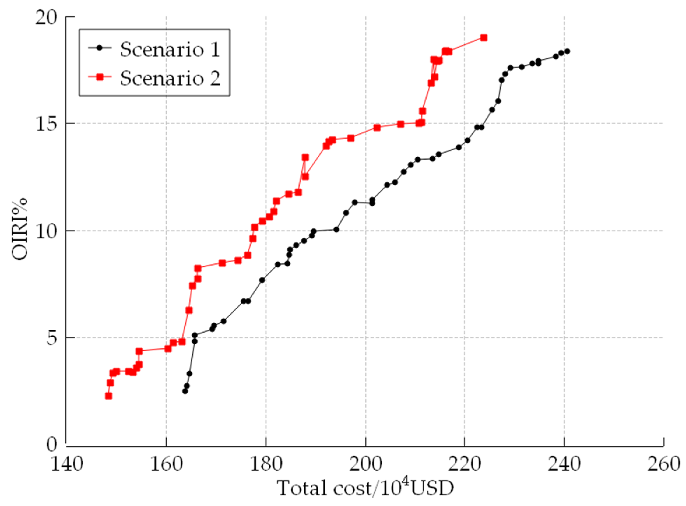
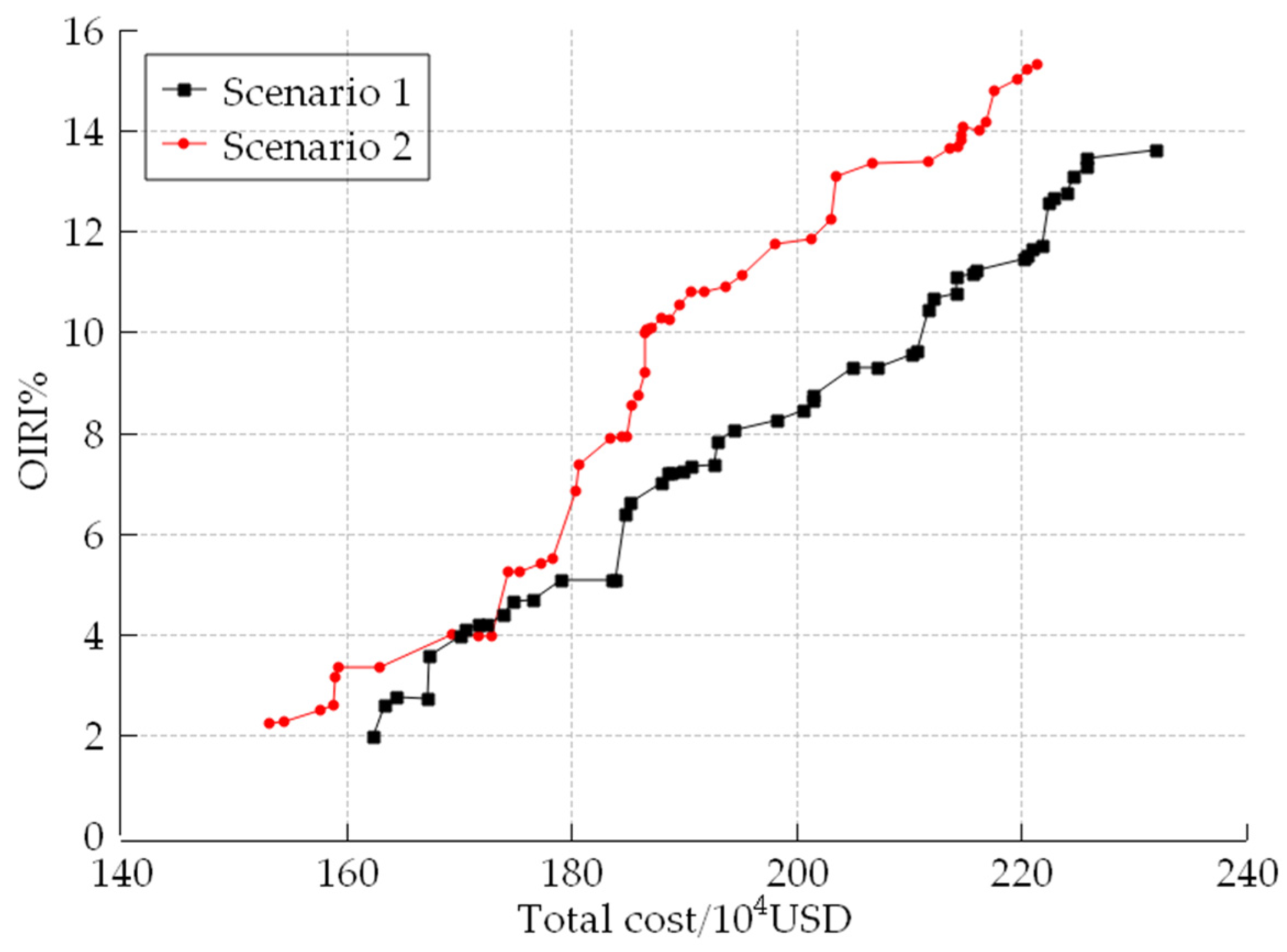
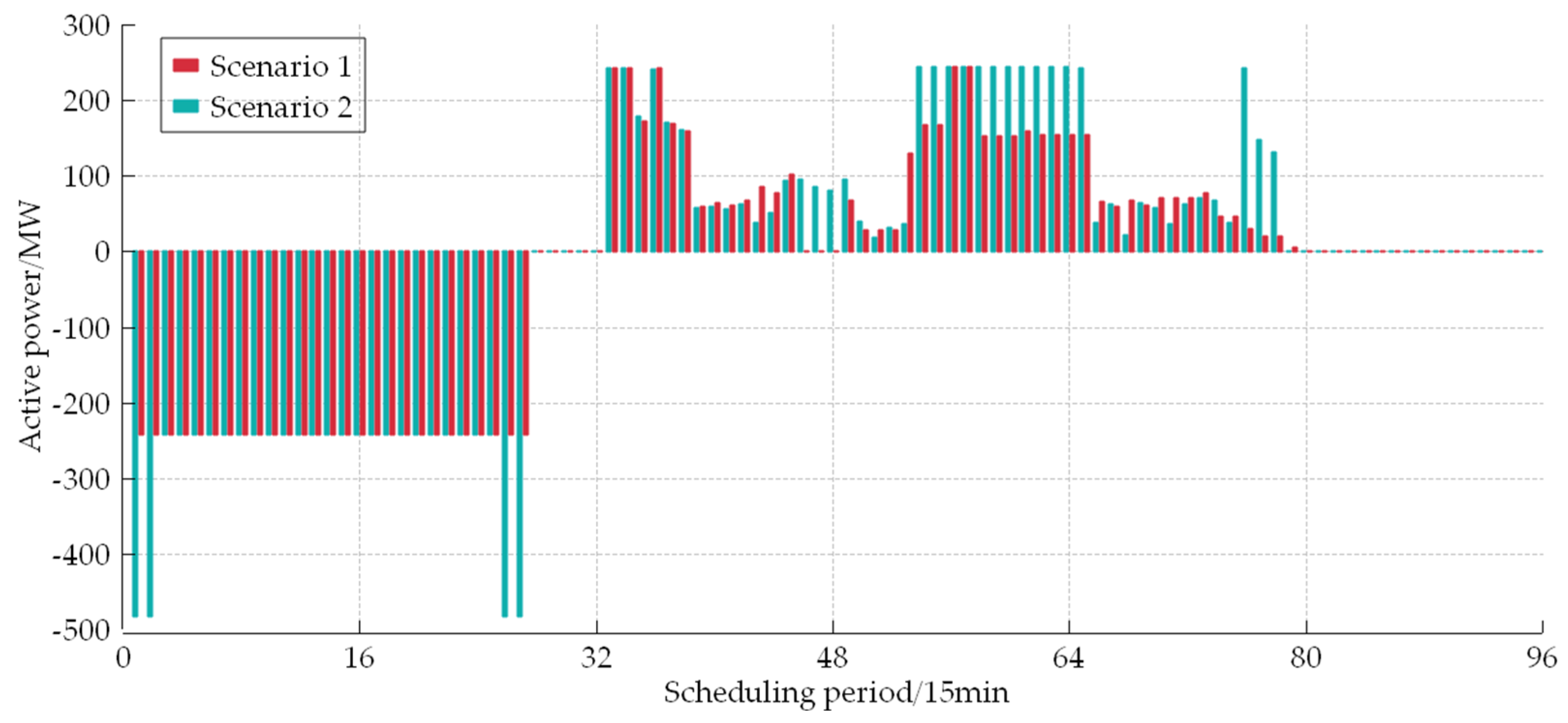
5.2. Inverse Robust Optimization Results Analysis

The daily power load and wind power output are depicted in Figure 4 and Figure 5, respectively. It is observed that the predicted wind power exceeds the actual wind power, leading to wind curtailment during practical operation. The primary reason for wind curtailment is that during certain periods, such as from 00:00 to 06:30, the load demand is relatively low, and the power systems’ capacity to accommodate wind power is insufficient.

Due to the requirement for PSHs to operate at rated power during pumping mode, only one or two PSHs can be in operation from 00:00 to 06:30. In light of these constraints, two scenarios are considered, and the inverse robust optimization approach is employed to find optimal solutions for them.

Scenario 1: Schedule one PSH to operate at full capacity during the specified time period (00:00 to 06:30). During other time intervals, the PSH can transition to power generation mode based on the specific optimization conditions.

Scenario 2: Flexibly schedule one or two PSHs to operate at full capacity based on the actual optimization conditions during the specified time period (00:00 to 06:30). During other time intervals, the PSHs can transition to power generation mode based on the specific optimization conditions.

As shown in Figure 6 and Figure 7, a comparison is provided between Scenario 1 and Scenario 2 in terms of the total generation cost and the OIRI with the ideal disturbance coefficients $\epsilon =$ 0.05 and $\epsilon =$ 0.10, respectively. Each set includes 50 Pareto optimal solutions. When the ideal disturbance coefficient is set to 0.05, the non-dominated front obtained by Scenario 2 outperforms that of Scenario 1. It indicates that when the ideal disturbance coefficient is set to 0.10, its relatively loose constraints on the objective function enhance the solution set’s robustness, thereby validating the rationality of the inverse robust optimization model proposed in this paper. The following analysis focuses solely on cases where the ideal disturbance coefficient is restricted to 0.10.

In

Table 2. Comparison of optimum of OIRI and cost.

	OIRI (max)	f/104 USD	OIRI	f(min)/104 USD
Scenario 1	17.48%	247.82	0.018%	164.09
Scenario 2	20.01%	232.59	0.027%	147.20

, the maximum wind power fluctuation that the system can withstand is OIRI (max), and the minimum total power generation cost is f (min). The results show the constraint relationships between the wind power accommodation and the total generation cost. In Scenario 1, when the ideal disturbance coefficient is 0.1, the wind power can be completely consumed as long as the error of wind power prediction is lower than 17.48%. The total generation cost under the maximum wind power forecasting deviation is USD 247.82 × 10⁴. In Scenario 2, wind power can be fully consumed when its prediction deviation is within 20.01%. Additionally, at the maximum wind power prediction deviation, the total generation cost is USD 232.59 × 10⁴.

The results of the optimization indicate that the maximum wind power prediction error that the system can tolerate can be determined based on the OIRI value, when operators have specific requirements for the total operating cost. If the wind power prediction error is large and the requirement for the total cost is low, the system may not be able to fully integrate wind power. For instance, when the wind prediction error is 0.15, both Scenario 1 and Scenario 2 require operating costs of around USD 225 × 10⁴ to achieve complete wind power absorption. On the other hand, lower operating costs can be achieved when the wind power prediction deviation is smaller. If the wind power prediction deviation is 0.05, the minimum operating cost is USD 180 × 10⁴. It is clear that if the grid follows Scenario 2 in scheduling, it will achieve complete integration of wind power with lower overall generation costs.

Figure 8 illustrates the daily working state curves of the PSHs under both scenarios. It is evident that the proposed inverse robust scheduling optimization strategy ensures the complete consumption of wind power. Additionally, Scenario 2 is more cost-effective than Scenario 1. The primary reason is that in Scenario 2, the PSHs absorb more wind power during the pumping stage, providing more flexibility in selecting output plans during the power generation periods.

5.3. Indictor Comparison Analysis

The WCSR is often used to represent the maximum hypersphere radius that ensures the robustness of the non-dominated solution set. The comparison between WCSR and OIRI is employed below to illustrate that compared to conventional interval quantification methods for robustness, OIRI can achieve better economy when addressing optimization scheduling problems affected by wind power uncertainties. WCSR can be calculated as follows:

$$WCSR=\min {\displaystyle \sum _{t=1}^T{‖{\mathit{P}}_t^w-{\mathit{P}}_t^{w_0}‖}_2}$$

(34)

Based on the data presented in

Table 3. Comparison between OIRI and WCSR methods.

Classification	Conventional Method	Scenario 1		Scenario 2
		OIRI	WCSR	OIRI	WCSR
the total cost/104 USD	276.41	225.60	229.04	192.11	203.91
coal consumption cost/104 USD	233.15	193.74	220.62	185.94	197.45
wind power penalty cost/104 USD	31.94	0	5.04	0	0
pumped storage start–stop cost/104 USD	11.32	2.9	2.9	5.76	5.76
pumped storage penalty cost/104 USD	0	0.29	0.48	0.41	0.69
wind curtailment/MWh	4487.16	0	708.45	0	0
CPU time (s)	153.1	219.9	253.9	228.4	261.7

, the OIRI method achieves full integration of wind power regardless of whether Scheme 1 or Scheme 2 is adopted. When the WCSR method is employed under Scheme 1, full integration of wind power cannot be achieved, and the total generation costs are higher. Under Scheme 2, although the WCSR method can fully integrate wind power, its total generation costs are higher compared to the results obtained using the OIRI method. Traditional scheduling methods do not take into account uncertainty and usually need less computation time compared to the algorithm considered in OIRI. However, the proposed algorithm has the ability to identify schedules that are lower in cost and can integrate more wind power. Moreover, its computation time is less than 5 min, which is within an acceptable range.

5.4. Large-Scale System Testing

The proposed method was compared with some commonly used heuristic methods, such as the non-dominated sorting genetic algorithm (NSGA) [22], multi-objective particle swarm optimization (MOPSO) [23], niched Pareto genetic algorithm (NPGA) [24], and strength Pareto evolutionary algorithm (SPEA) [25]. These methods have been successfully applied to optimize economic dispatch. Their performances were evaluated by testing a modified IEEE 118-bus system whose detailed parameters are available online at http://motor.ece.iit.edu/data (accessed on 1 January 2023). The system consists of 118 buses, 33 generators, and 186 transmission lines. Based on the original IEEE 118-bus system, two wind farms and two pumped storage power stations were added at bus 12 and 61, respectively. Each pumped storage power station has a capacity of 270 MW. The forecasted wind power can be found in reference [14].

The results of the simulation are summarized in

Table 4. Comparison between different heuristic methods and OIRI index.

	Proposed Method	NSGA	MOPSO	NPGA	SPEA
the total cost/104 USD	309.21	352.62	316.19	316.42	315.81
coal consumption cost/104 USD	299.28	319.24	306.03	306.21	306.61
wind power penalty cost/104 USD	0	0	0	0	0
pumped storage start–stop cost/104 USD	9.27	31.92	8.97	8.95	8.97
pumped storage penalty cost/104 USD	0.66	1.46	1.19	1.26	0.23
wind curtailment/MWh	0	0	0	0	0
CPU time (s)	542.4	549.8	590.7	560.1	571.3

. To ensure a fair comparison between the different approaches, ten optimization runs were conducted, and the average values are shown. It was found that the proposed method has the lowest total cost and the shortest computation time. All of the methods tested were able to fully integrate wind power using PSHs and the OIRI index. Compared to the previous 42-bus test system, the number of thermal units in the modified IEEE 118-bus system increased from 22 to 33, and finding the optimal economic dispatch plan is a critical factor in reducing costs. The proposed algorithms were able to find better scheduling schemes for both thermal units and PSHs when wind power was fully integrated. This resulted in reduced coal generation costs of thermal units and start–stop costs of PSHs.

6. Conclusions

To integrate wind power efficiently and minimize electricity generation costs, we propose a bi-level inverse robust wind power–PSHs optimization scheduling model. The model is solved using a combination of the grid multi-objective bacterial colony chemotaxis algorithm and the bisection method. This paper introduces an inverse robust indicator, which not only addresses the limitations of pumped storage in mitigating wind power fluctuations but also establishes the relationship between the maximum forecast deviation and the minimum generation cost associated with each non-dominated solution in the optimal load allocation. Case studies on operational data from a specific regional power grid validate the proposed method. Two optimization scenarios are developed and compared with the actual operation data. The case studies indicate that optimizing the pumping and generation operation of PSHs addresses the limitations of accommodating wind power. The proposed method enhances both economic efficiency and wind power consumption. It provides a clear relationship between the objective function and decision vectors, offering valuable insights for developing robust scheduling plans.

References

1. Zhao, J.F.; Oh, U.J.; Park, J.C.; Park, E.S.; Im, H.B.; Lee, K.Y.; Choi, J.S. A Review of World-wide Advanced Pumped Storage Hydropower Technologies. IFAC-Pap. 2022, 55, 170–174. [Google Scholar] [CrossRef]
2. Javed, M.S.; Ma, T.; Jurasz, J.; Amin, M.Y. Solar and Wind Power Generation Systems with Pumped Hydro Storage: Review and Future Perspectives. Renew. Energy 2020, 148, 176–192. [Google Scholar] [CrossRef]
3. Yuan, W.Y.; Xin, W.P.; Su, C.G.; Cheng, C.; Yan, D.; Wu, Z. Cross-regional Integrated Transmission of Wind Power and Pumped-Storage Hydropower Considering the Peak Shaving Demands of Multiple Power Grids. Renew. Energy 2022, 190, 1112–1126. [Google Scholar] [CrossRef]
4. Hu, Z.J.; Zhang, M.L.; Wang, X.F.; Li, C.; Hu, M.Y. Bi-level Robust Dynamic Economic Emission Dispatch Considering Wind Power Uncertainty. Electr. Power Syst. Res. 2016, 135, 35–47. [Google Scholar] [CrossRef]
5. Bentsen, L.; Warakagoda, N.D.; Stenbro, R.; Engelstad, P. Relative Evaluation of Probabilistic Methods for Spatio-Temporal Wind Forecasting. J. Clean. Prod. 2024, 434, 139944. [Google Scholar] [CrossRef]
6. Tang, C.H.; Xu, J.; Tan, Y.S.; Sun, Y.Z.; Zhang, B.S. Lagrangian Relaxation with Incremental Proximal Method for Economic Dispatch with Large Numbers of Wind Power Scenarios. IEEE Trans. Power Syst. 2019, 11, 436–447. [Google Scholar] [CrossRef]
7. Xu, X.; Yan, Z.; Shahidehpour, M.; Li, Z.; Yan, M.; Kong, X. Data-Driven Risk-Averse Two-Stage Optimal Stochastic Scheduling of Energy and Reserve with Correlated Wind Power. IEEE Trans. Sustain. Energy 2020, 27, 206–215. [Google Scholar] [CrossRef]
8. Wu, C.Y.; Wei, G.; Zhou, S.Y.; Chen, X.G. Coordinated Optimal Power Flow for Integrated Active Distribution Network and Virtual Power Plants Using Decentralized Algorithm. IEEE Trans. Power Syst. 2021, 36, 3541–3551. [Google Scholar] [CrossRef]
9. Ran, X.H.; Zhang, J.H.; Zhu, W.J.; Liu, K.P.; Liu, Y.S. A Model of Correlated Interval–Probabilistic Conditional Value-at-Risk and Optimal Dispatch with Spatial Correlation of Multiple Wind Power Generations. Int. J. Electr. Power Energy Syst. 2024, 155, 109500. [Google Scholar] [CrossRef]
10. Wang, Z.N.; Fang, G.H.; Wen, X.; Tan, Q.F.; Zhang, P.; Liu, Z.H. Coordinated Operation of Conventional Hydropower Plants as Hybrid Pumped Storage Hydropower with Wind and Photovoltaic Plants. Energy Convers. Manag. 2023, 277, 116654. [Google Scholar] [CrossRef]
11. Soyster, A.L. Convex Programming and Set-Inclusion Constraints and Applications to Inexact Linear Programming. Oper. Res. 1973, 21, 1154–1157. [Google Scholar] [CrossRef]
12. Ahmed, S.; Sahinididis, N.V. Robust Process Planning under Uncertainty. Ind. Eng. Chem. Res. 1998, 37, 1883–1892. [Google Scholar] [CrossRef]
13. Jin, Y.C.; Branke, J. Evolutionary Optimization in Uncertain Environments-A Survey. IEEE Trans. Evol. Comput. 2005, 9, 303–317. [Google Scholar] [CrossRef]
14. Zhao, C.Y.; Wang, J.H.; Watson, J.P.; Guan, Y.P. Multi-Stage Robust Unit Commitment Considering Wind and Demand Response Uncertainties. IEEE Trans. Power Syst. 2013, 28, 2708–2717. [Google Scholar] [CrossRef]
15. Xiong, H.B.; Shi, Y.H.; Chen, Z.; Guo, C.X.; Ding, Y. Multi-Stage Robust Dynamic Unit Commitment Based on Pre-Extended—Fast Robust Dual Dynamic Programming. IEEE Trans. Power Syst. 2023, 38, 2411–2422. [Google Scholar] [CrossRef]
16. Wu, W.C.; Chen, J.H.; Zhang, B.M.; Sun, H.B. A Robust Wind Power Optimization Method for Look-Ahead Power Dispatch. IEEE Trans. Sustain. Energy 2014, 5, 507–515. [Google Scholar] [CrossRef]
17. Zhang, R.F.; Chen, Y.; Li, B.X.; Jiang, T.; Li, X.; Chen, H.H.; Ning, R.X. Adjustable Robust Interval Economic Dispatch of Integrated Electricity and District Heating Systems under Wind Power Uncertainty. Energy Rep. 2022, 8, 13138–13149. [Google Scholar] [CrossRef]
18. Xu, M.; Li, W.W.; Feng, Z.H.; Bai, W.W.; Jia, L.L.; Wei, Z.H. Economic Dispatch Model of High Proportional New Energy Grid-Connected Consumption Considering Source Load Uncertainty. Energies 2023, 16, 1696. [Google Scholar] [CrossRef]
19. Gunawan, S.; Azarm, S. Multi-objective Robust Optimization Using A Sensitivity Region Concept. Struct. Multidiscip. Optim. 2005, 29, 50–60. [Google Scholar] [CrossRef]
20. Lu, Z.; Zhao, H.; Xiao, H.F.; Wang, H.R.; Wang, H.J. An Improved Multi-Objective Bacteria Colony Chemotaxis Algorithm and Convergence Analysis. Appl. Soft Comput. 2015, 31, 274–292. [Google Scholar] [CrossRef]
21. Lu, Z.; Feng, T.; Li, X.P. Low-carbon Emission/Economic Power Dispatch Using the Multi-Objective Bacterial Colony Chemotaxis Optimization Algorithm Considering Carbon Capture Power Plant. Int. J. Electr. Power Energy Syst. 2013, 53, 106–112. [Google Scholar] [CrossRef]
22. Basu, M. A Nondominated Sorting Genetic Algorithm III with Three Crossover Strategies for the Combined Heat and Power Dynamic Economic Emission Dispatch with or without Prohibited Operating Zones. Eng. Appl. Artif. Intell. 2023, 123, 106443. [Google Scholar]
23. Zhang, Q.; Ding, J.J.; Shen, W.X.; Ma, J.H.; Li, G.L. Multiobjective Particle Swarm Optimization for Microgrids Pareto Optimization Dispatch. Math. Probl. Eng. 2020, 2020, 5695917. [Google Scholar] [CrossRef]
24. Abido, M.A. A Niched Pareto Genetic Algorithm for Multiobjective Environmental/Economic Dispatch. Int. J. Electr. Power Energy Syst. 2003, 25, 97–105. [Google Scholar] [CrossRef]
25. Jiang, S.Y.; Yang, S.X. A Strength Pareto Evolutionary Algorithm Based on Reference Direction for Multiobjective and Many-Objective Optimization. IEEE Trans. Evol. Comput. 2017, 21, 329–346. [Google Scholar] [CrossRef]
Figure 1. Flow chart of the multi-objective bacterial colony chemotaxis algorithm.
Processes 12 00729 g001
Figure 2. Flow chart of solution procedure.
Processes 12 00729 g002
Figure 3. Schematic diagram of network topology.
Processes 12 00729 g003
Figure 4. The predicted power load and actual power load.
Processes 12 00729 g004
Figure 5. The predicted wind power and actual wind power.
Processes 12 00729 g005
Figure 6. The results of OIRI and total generation cost (ideal disturbance constraint for 0.05).
Processes 12 00729 g006
Figure 7. The results of OIRI and total generation cost (ideal disturbance constraint for 0.1).
Processes 12 00729 g007
Figure 8. Working states of PSHs under different schemes.
Processes 12 00729 g008