Article

Fully Coupled CFD–DEM Simulation of Oil Well Hole Cleaning: Effect of Mud Hydrodynamics on Cuttings Transport

by
Alireza Zakeri
1,
Mohammadreza Alizadeh Behjani
2 and
Ali Hassanpour
1,*
1
School of Chemical and Process Engineering, University of Leeds, Leeds LS2 9JT, UK
2
School of Chemistry and Chemical Engineering, University of Surrey, Guildford GU2 7XH, UK
*
Author to whom correspondence should be addressed.
Processes 2024, 12(4), 784; https://doi.org/10.3390/pr12040784
Submission received: 14 February 2024 / Revised: 22 March 2024 / Accepted: 25 March 2024 / Published: 13 April 2024
(This article belongs to the Section Particle Processes)

Abstract

:
This paper presents a coupled computational fluid dynamics–discrete element method (CFD–DEM) simulation to predict cuttings transport by the drilling fluid (mud) in different oil well drilling conditions. The mud rheology is expressed by the Herschel–Bulkley behaviour and modelled in a Eulerian framework (CFD), while the cuttings are modelled using the Lagrangian approach (DEM). In this work, the effects of drill string rotation, inclination angle, cutting size, mud rheology, and annular velocity on cleaning efficiency are investigated. It is found that increasing the well deviation from vertical to horizontal leads to a higher cuttings concentration. However, at low annular velocity, the cuttings concentration for the inclined (45-degree) annulus is found to be higher than the horizontal one due to the sliding motion of cuttings on the lower section of the annulus. Overall, the drill pipe rotation has little effect on decreasing the cuttings concentration, but the effect is more pronounced at low annular velocity.

1. Introduction

In oil and gas drilling, the term hole cleaning refers to the transport of the generated cuttings to the surface by circulating a drilling fluid, commonly known as mud, through the annulus of the wellbore. The cutting deposition in the direction of the gravitational force leads to formation of a cutting layer bed near the bottom section of the annulus. Formation of the cutting bed caused by inefficient hole cleaning leads to a slow drilling rate (rate of penetration) and consequently increases the cost of the drilling. In order to tackle this problem, it is essential to gain an in-depth understanding of the mud hydraulics and identification of influencing parameters that control the hole cleaning efficiency.
The most relevant parameters that affect the cleaning efficiency can be listed as: (1) annular fluid velocity profile, (2) mud properties, (3) hole inclination angle, (4) mud annular velocity, (5) drill pipe/string eccentricity, (6) penetration rate, and (7) drill pipe/string rotation. The challenges associated with transporting the cuttings have been investigated by numerous experimental studies (e.g., Udo Zeidler [1]; Tomren et al. [2]; Brown et al. [3]; Penden et al. [4]; Sifferman et al. [5]; Bassal, A.A. [6]; Sanchez et al. [7]; Yu et al. [8]). Experimental investigations provide a comprehensive study on the cuttings concentration in simulated well conditions in laboratory conditions; however, in real well conditions, considering operational limitations and boundaries besides unexpected situations that typically occur during the drilling processes, it is difficult and very expensive to create a well-designed and controlled full-scale laboratory rig. A reliable numerical simulation can help to understand the hole cleaning process while investigating the effects of various key parameters in cuttings transport simultaneously.
Many researchers have investigated the cuttings transport performance in directional well drilling using modelling and simulation techniques (e.g., Bilgesu et al. [9,10]; Wang et al. [11]; Yilmaz [12]; Rooki et al. [13]; Mohammadzadeh et al. [14]; Amanna et al. [15]; Tong et al. [16]). Computational fluid dynamics (CFD) has been used in the majority of these studies, mainly in a Eulerian framework, to assess the impact of different parameters on the cleaning efficiency of oil well drilling operations. The major drawback of the CFD simulations is the difficulty in accurately modelling the solid phase (cuttings). For example, Rooki et al. [13] developed a two-phase fluid model (TFM) to study the impact of mud properties on cuttings transport mechanisms. Since the cuttings are treated as a continuous phase in a Eulerian–Eulerian framework, their true discrete characteristic information could not be easily modelled. Yilmaz [12] studied the impact of mud properties, well inclination angle, and pipe rotation speed on cuttings transport using the discrete dense particle method (DDPM) based on a two-way coupling approach. DDPM (Lagrangian–Eulerian) overcomes the TFM limitations and allows to track solid particles individually or grouped (parcels) according to Newton’s second law of motion. However, in DDPM the particle–particle interaction is not accurately modelled and can be more applicable for a dilute system. The most appropriate approach to model the hole-cleaning process in oil wells is fully coupled CFD–discrete element method (DEM). A few studies have considered this approach, addressing the common issues with the transport of rock fragments during the drilling operation [17,18,19,20]. For example, the effect of mud flow rate, inclination angle, well pressure, and raised temperature on the cuttings transport efficiency in a concentric annulus for an aerated mud drilling process were studied by Akhshik et al. [20]. In another work, the effect of drill pipe rotation on cuttings transport behavior has been investigated using the CFD–DEM approach [17]. The impact of the microscopic properties of particles, such as the sliding and rolling friction coefficients of particle–particle, particle–drill string, and particle–wall contact interactions on the characteristics of cuttings transport mechanisms near a horizontal deviated well was investigated [19]. It was reported that the sliding friction coefficient has a dominant role in cuttings transport in comparison with the rolling friction factor. It should be noted that in the work by Akhshik et al. [19], the particle size and the hydraulic diameter were 6.35 mm and 78 mm (annular distance of 36 mm), respectively. No information on the mesh size nor a clear mesh dependency study was reported, but considering the approach requires a mesh size about two times (or more) bigger than the particle diameter, the number of meshes (relatively coarse) should have been very limited across the annulus. Moreover, considering the turbulence of the carrier phase (fluid), the velocity gradient near the wall was significantly high, and the simulation results tend to be influenced by the mesh size [21].
The use of CFD–DEM requires careful consideration of particle–fluid interactions, particularly considering appropriate mesh configurations, which would be computationally very expensive for fully resolved systems. Hence, approximations based on unresolved systems, where mesh size should be larger than particles, need careful attention, particularly for investigating particle behavior near the wall conditions. Most of the recent studies are suffering from lack of mesh refinement for particle–fluid interactions near the wall region, which is significantly important for the sedimentation and suspension of cuttings. Overall, a systematic study of the effect of mud rheology on cuttings transport in fully coupled CFD–DEM with appropriate mesh configuration near wall regions is still lacking in the literature. The aim of this paper is therefore to simulate The cuttings transport process in the bottomhole using a fully coupled CFD–DEM approach. In this work, we use optimized mesh refinement to account for the wall effects. The impact of mud rheology, cutting size, drill rotation, inclination angle, and mud annular velocity on the cuttings transport and the hole cleaning efficiency are investigated.

2. Model Description

A three-dimensional (3D) model of an annulus of an oil well was simulated to study the cuttings transport in vertical, deviated, and horizontal well drillings using fully coupled CFD–DEM. The mud (the continuous phase) motion is modelled as an incompressible fluid based on a Eulerian CFD approach and the cutting (dispersed solid phase) collisions are simulated by the DEM method. The continuous fluid and discrete solid phases are fully coupled via interaction forces (e.g., drag force, lift force). The mathematical formulation for modelling of each phase is presented in the following section.

2.1. Fluid Phase Modelling

The governing equations of motion of unsteady, viscous, and incompressible fluid phases can be described by the Reynolds averaged Navier–Stokes equations (RANS) as follows:
( α ρ f ) t + · α ρ f u f = 0
where u f is the fluid velocity, ρ f is the fluid density, and   α   is the volume fraction of the fluid phase. The momentum conservation equation is expressed as:
α ρ f u f t + · α ρ f u f u f = α p + α · τ S f + α ρ f g
where p is the fluid pressure, τ is the viscous stress tensor, and S f is the volume-averaged interaction force. For a particular computational cell, the source term force, S f , is obtained using the following equation:
S f = i = 1 M F f , i V c e l l
where M is the number of particles, Ff,i is the force from particle i, and V c e l l is the volume of fluid in the computational cell.
In oil well drilling operations, the mud follows non-Newtonian fluid properties. It has been suggested that the Herschel–Bulkley model better agrees with the rheological performance of drilling fluids [22], and it can approximate the mud viscosity over a large range of shear rates. The dynamic viscosity in the Herschel–Bulkley model is expressed using Equation (4):
μ = μ y i e l d             i f   γ ˙ < τ 0 μ y i e l d μ = τ 0 + k ( γ ˙ n ( τ 0 μ y i e l d ) n ) γ ˙       i f   γ ˙ τ 0 μ y i e l d
where k is the consistency factor, n is the power law exponent,   μ y i e l d represents the yielding viscosity, τ 0 defines the yield stress threshold, and γ ˙ expresses the strain rate magnitude.

2.2. Solid Phase Modelling

2.2.1. Solid Phase Motion

The motion of each particle is simulated individually using Newton’s equations by considering the relevant forces acting on the particle p in a fluid flow using the following equation:
m p u p t = m p g 1 ρ f ρ p + i = 1 k c F c , i p + F D + F S + F M + F P +
where m p   and ρ p are the mass and density of particle p, respectively, F c , i p is the contact force acting on the external spherical element of the particle at element   i , k c refers to the number of spherical elements on the external surface of each particle (we assume all the particles are spherical in this study), F S is the shear lift force, F M is the rotational lift or Magnus force, and F P is the fluid pressure gradient force [23]. For the contact force calculations, we consider both particle–particle and particle–wall collision interactions according to the elastic contact behavior in absence of adhesion or cohesion, based on the Hertz–Mindlin (no-slip) model.
The rotational motion of particle p can be described as:
d d t I p ω p = e = 1 k c ( T t , e D + T r , e D ) + T D T p
where T D T p is the drag torque created by the slip rotation and T t , e D and T r , e D   ( e = 1 ,   2 , , k c ) are the torque vectors created by tangential and normal contact forces, respectively, acting on a particle p [24] with the moment of inertia I p and rotational velocity ω p .
Once the force has been calculated, the particle trajectories are obtained by means of integration of the particle velocity as follows:
d x p d t = u p
where xp and up the particle position and velocity at time t, respectively.

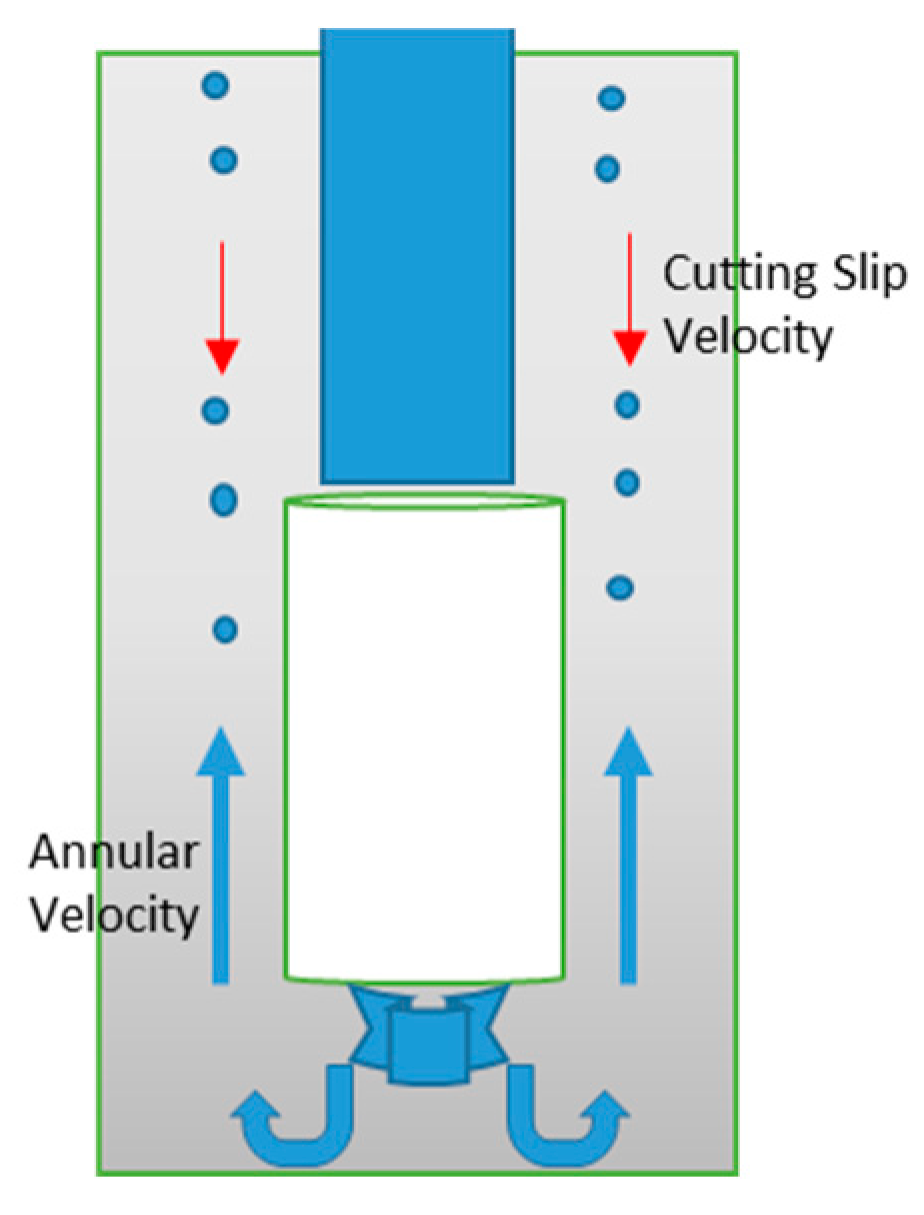
2.2.2. Cuttings Slip Velocity

Cuttings slip velocity is the velocity of particles relative to the adjacent fluid. For instance, while particles experience an upward force by drilling fluid velocity, inversely, gravity forces them downward (settling tendency of cuttings) (Figure 1). Therefore, in the cleaning process, mud flow velocity should be greater than cuttings slip velocity, otherwise the cleaning process fails.
Various equations have been derived to evaluate the slip velocities of spherical particles in different flow regimes. The applicability of theses equations depends on the particle Reynolds number:
R e p = ρ f d p V s μ
where particle Reynolds number ( R e p ) is a function of slip velocity ( V s ), diameter of particles ( d p ), viscosity ( μ ), and density ( ρ f ) of fluid.
The equation of motion for a spherical particle inside a viscous fluid is given below:
d u p d t = 18 μ f ρ p   D p 2   C D   R e p 24 ( u f u p )
where the drag force coefficient C D is obtained as follows [25]:
C D = 24 R e     i f   R e p < 1 24 R e p   1 + 0.15   R e p 0.687           i f   1 R e p 1000 0.44     i f   R e p > 1000
In turbulent flow, the drag coefficient becomes constant. Hence, slip velocity can be calculated by Zeidler’s [26] equation:
V s = 9   D p ( ρ p ρ f ) ρ f               R e p > 1000        
In the intermediate range of particle Reynolds number, applicable in this study, Stokes’ law can be used to obtain the slip velocity, as shown by Equation (12):
V s = 4 g D p ( ρ p ρ f ) 3 ρ f C D         1 < R e p < 1000
In Equation (9), for the lower limits of Reynolds numbers, CD  1 , the velocity response time can be obtained from Equation (13):
τ p = ρ p D p 2 18 μ f
which is used to characterize the capability of particles to follow velocity changes in the flow.
The Stokes number is a very important parameter related to the particle velocity. It can be defined as the particle response time over the characteristic time scale of the flow using the following correlation:
S t = τ p τ f
where the characteristic time of flow field ( τ f ) can be defined as:
τ f = l u f
where the length scale ( l ) in this study would be the hydraulic diameter ( D h ) . Hence, Equation (15) can be rewritten as:
S t = τ p u f D h
If St ≤ 1, the particle response time is much less than the characteristic time associated with the flow field. As a result, the particle has sufficient time to respond to changes in flow velocity. Consequently, the particle and fluid velocities will reach velocity equilibrium. Conversely, if St ≥ 1, the particle has no time to respond to changes in flow velocity, and the particle velocity will be unaltered.

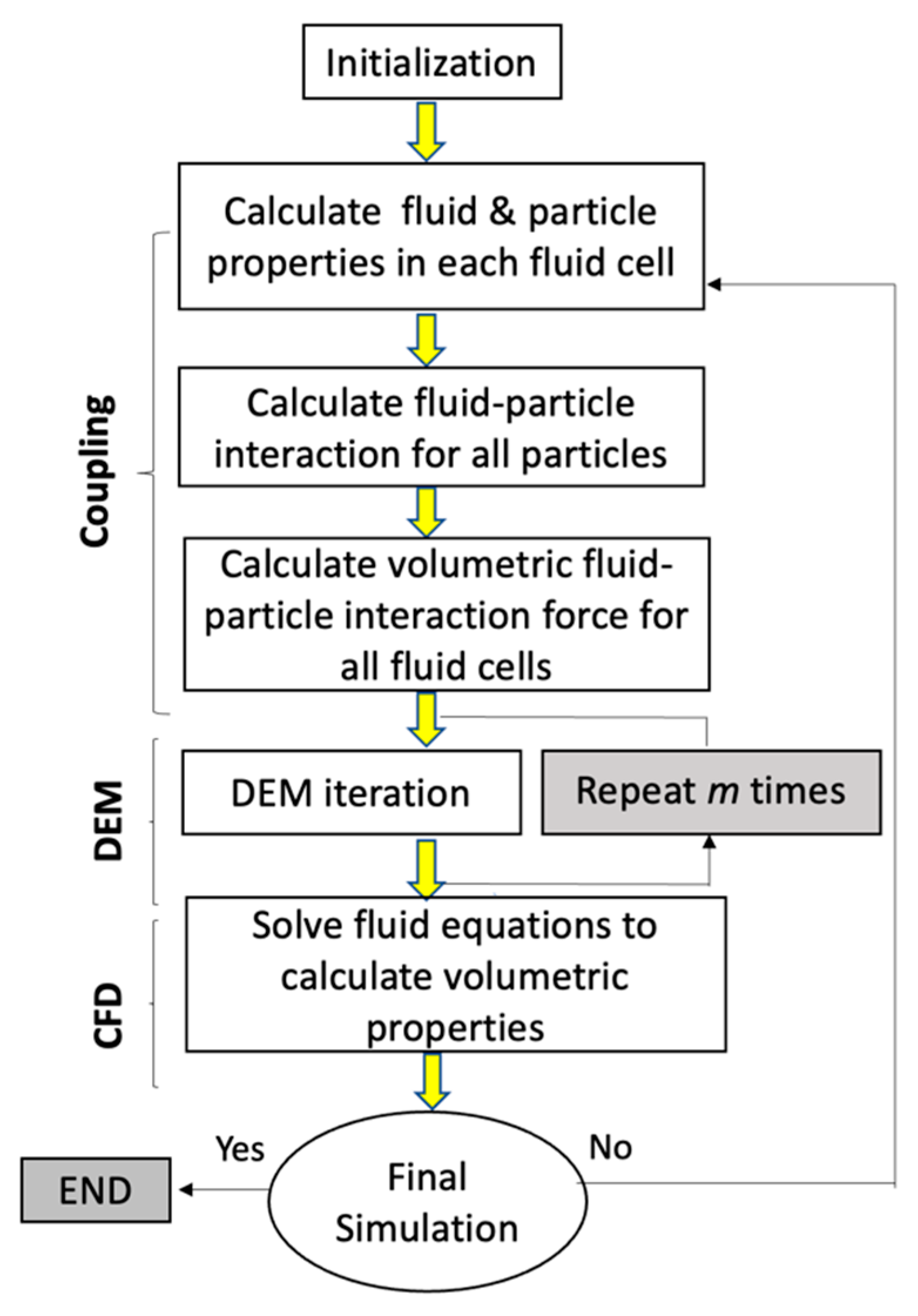
2.3. CFD–DEM Coupling

Figure 2 illustrates a diagram of the CFD–DEM framework. The ANSYS fluent CFD code is coupled to the EDEM 2022.1 software (Altair Engineering) via adding a user defined function (UDF) file to the coupling interphase library. It can be observed that the calculation process begins with the initialization of all components of the simulation. Based on the position of the particles and mesh information, the fluid properties are calculated in each fluid cell and transferred to the coupling phase. Furthermore, the fluid–particle interaction force acting on each particle is calculated using the information at current fluid time steps. Moreover, the volumetric fluid–particle interaction force in each fluid cell is calculated. The next step consists of the iteration loop of the DEM. The data from the coupling phase is used in the equation of the motion of each particle. The iteration loop of DEM is repeated m times (here, the DEM time step is typically 10 2 times smaller than the CFD time step). Next, after the DEM loop completion, the new information of all particles is calculated at the next fluid time step. In CFD, all fluid phase equations are used to obtain volumetric fluid–particle interactions. The CFD solver iterates over the next time step until the solution converges in sequence of calculations.

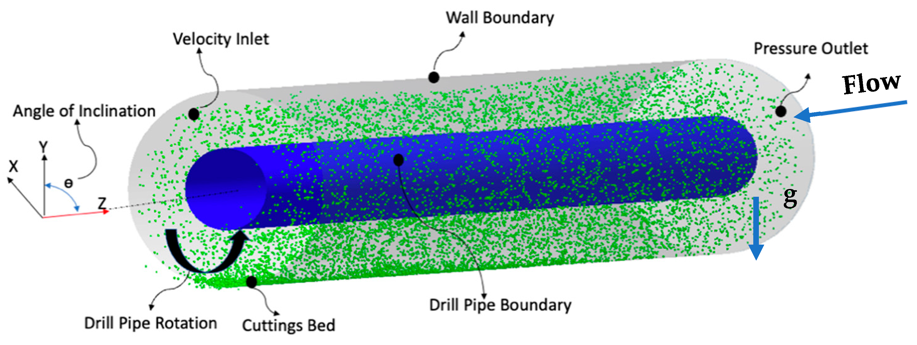
2.4. Model Geometry and Boundary Conditions

The model is considered as a confined-length concentric annulus consisting of two cylindrical bodies. The interior cylinder represents the drill pipe and rotates with a constant angular velocity around its axis. In real drilling conditions, the mud is injected through the drill string all the way to the drill bit and is exerted from the nozzles of the bit, followed by flushing the cuttings from the bottomhole and transferring drill cuttings to the surface through the annulus. In the drilling process, the length of the annulus can be thousands of meters, in which the drill string is placed. In order to reduce the computational cost, a section of the annulus with fully developed length is modelled [26]. In this work we assume that this annulus is very close to the drill bit; hence, a known number of cuttings per second (based on rate of drilling) are constantly generated and enter the annulus, where they can be ejected/flushed from the other end. The length of the annulus ( l ) is selected in a way to ensure fully developed turbulent fluid flow within the annulus at a different Reynolds number ( l > 20 D ) [27]. A concentric annulus with an outer diameter of 120 mm and an inner diameter of 50 mm with a 1500 mm length is modelled as presented in Figure 3. In this work, we employed the Reynolds stress model (RSM) to account for the turbulence regime.
Two-phase (particle–fluid) flow with uniform bulk velocity and uniform cutting fluid volume fraction enters the annulus from one end and exits from the other end. Boundary conditions were considered as the inlet flow velocity and the ambient pressure outlet. The process is isothermal, and the wall boundary (contact between particles and walls) was treated as a no-slip condition. Particles were generated at the inlet with the same velocity as the inlet fluid. In this study, 10,000 particles per second are injected into the system where the particle density is 2600 kg/ m 3 . This corresponds to the cuttings mass flow rate of 0.037 kg/s, calculated based on the representative rate of penetration (ROP) of 4.57 m/h (15 ft/h). The rheological properties, geometrical characteristics, and simulation input parameters in this study are shown in Table 1.

2.5. Relative Cuttings Concentration

Sifferman et al. [28] defined the cuttings transport efficiency as the ratio of the average cuttings transport velocity to the average fluid velocity. In this study, a different concept is defined to investigate the cuttings transport capacity of mud. The ratio of the number of remained particles in the annulus (until reaching steady state) over the total number of particles injected into annulus is defined as relative cuttings concentration (RCC):
R C C = N u m b e r   o f   p a r t i c l e s   r e m a i n e d   i n   a n n u l u s T o t a l   n u m b e r   o f   i n j e c t e d   p a r t i c l e s
A lower RCC would refer to a better cleaning performance. In this study, RCC needs to be distinguished from the absolute cuttings concentration, which is the ratio of the volume of remaining particles to the total volume of the annulus at steady state.

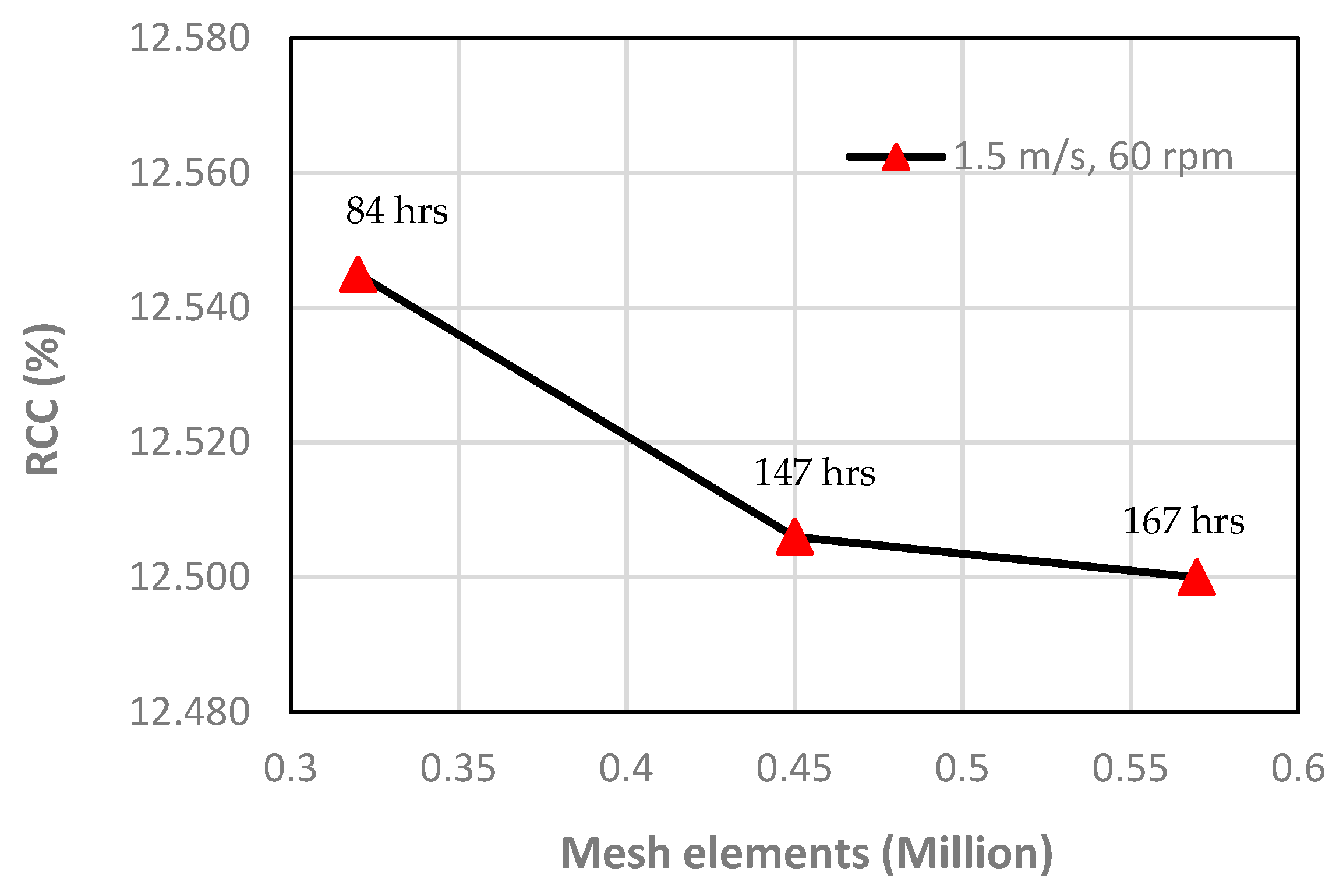
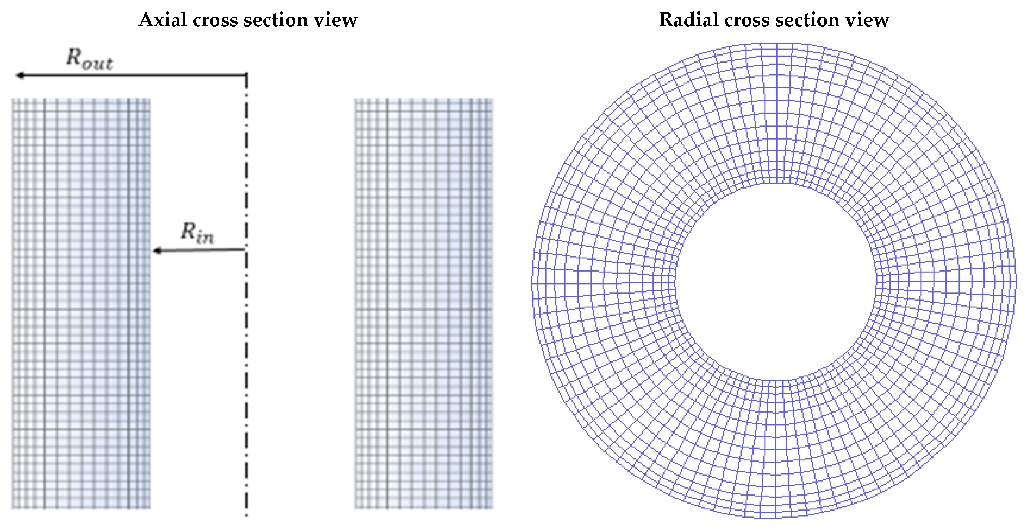
2.6. Mesh Information

The discretization of the computational domain is preformed based on the fluid phase calculations. It should be also noted that for the unresolved CFD–DEM modelling, the grid size must be larger than the largest particle in the domain. To obtain the optimum mesh arrangement with the minimum number of computational cells, a mesh sensitivity study is usually carried out prior to running the main simulations. In this work, the RCC results of a vertical well with 1.5 m/s mud velocity were obtained using different number of mesh elements. In Figure 4, the steady state RCC and the required computational efforts (using the Intel® Xeon® @ 3.10 GHz workstation with 24 cores and 64 GB of RAM) is plotted against the mesh number. It can be seen that the cuttings concentration slightly decreases as the mesh number is increased. This could be due to the fact that a smaller mesh size (due to higher number of meshes) could result in more accurate representations of fluid–particle interactions, leading to more particles being transported by fluid in the annulus. It can be also observed that the change in cuttings concentration from 450,000 to 569,710 mesh cells is very small. It was not possible to increase the mesh number beyond 569,710 as this would result in mesh sizes being equal or smaller than particle sizes, which is not compatible with the unresolved CFD–DEM principles.
Based on the results in Figure 4, with respect to particle size, grid size limitation, and computation effort, the 569,710-cell mesh configuration was chosen. The computational cells on the axial and radial cross sections of the annulus are presented in Figure 5.

2.7. Mud Properties

Simulations were carried out for fully developed fluid–solid phase flow in a vertical (0°) and deviated annuli (45° & 90°), where muds with different rheological properties, i.e., low, intermediate, and high viscosities, were used. The mud properties shown in Table 2 were selected based on the experimental studies of Tomren [2] and Okranji and Azar [29]. The mud was considered as a Hershel–Bulkley non-Newtonian fluid, as discussed previously in the methodology section.

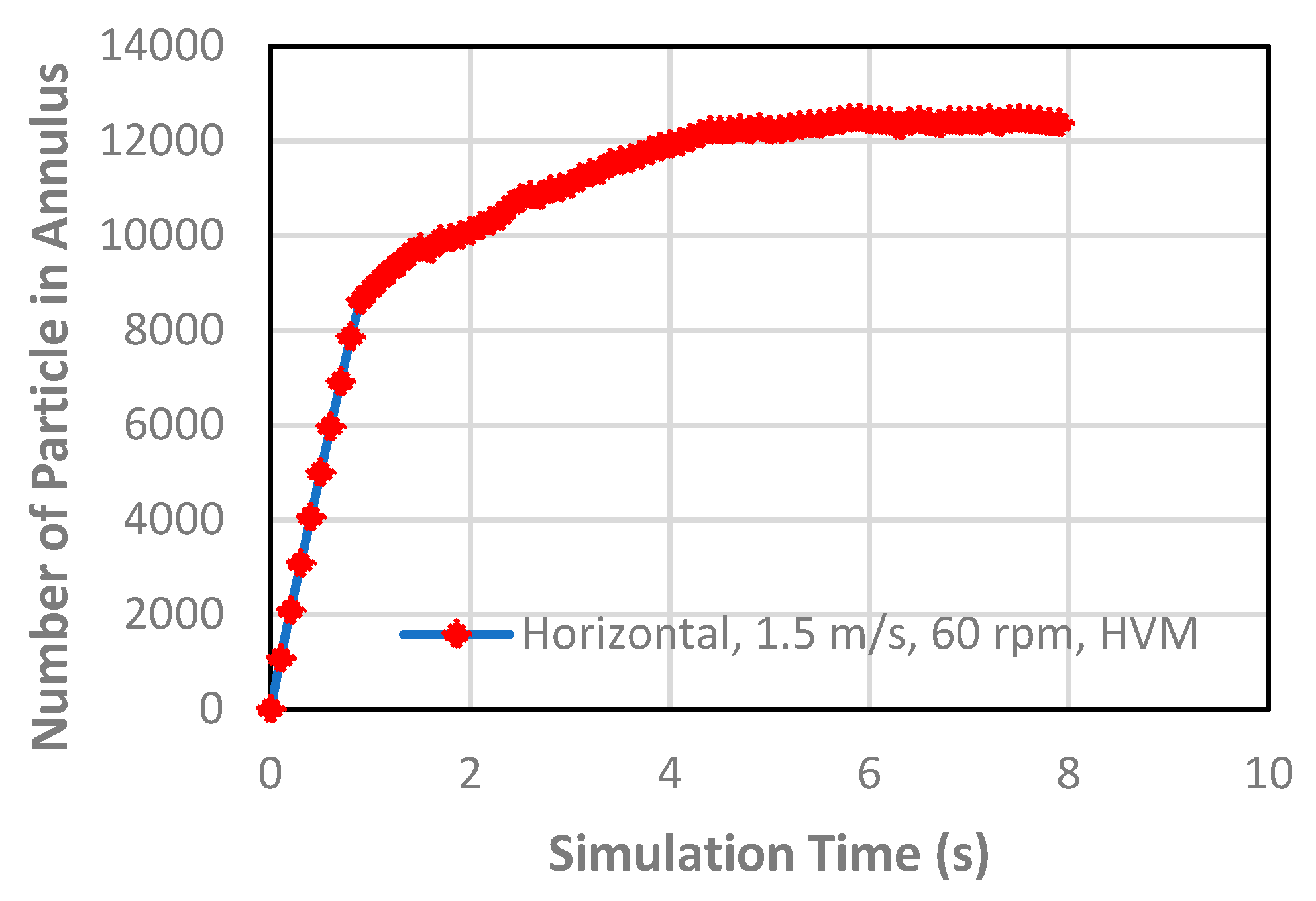
2.8. Steady State Condition

For a typical case, the evolution of number of particles in the annulus as a function of simulation time is plotted in Figure 6. In this figure, the results are shown for a horizontal wellbore with high viscosity mud (HVM) and annular velocity of 1.5 m/s with an average particle size of 1.4 mm, while the pipe is rotated at 60 rpm. It can be seen that there is an initially linear correlation between number of particles and time, which is similar to the rate of particle injection (10,000 particles/second). After about 0.8 s, the number of particles in the annulus starts to level off and reaches the steady state at around 4.5 s, where a relatively constant particle number in the annulus, corresponding to a solid fraction of about 0.00128, was achieved for this case.
In the following section, the impact of mud flow rate, rheology, inclination angle, and drill pipe rotation speed on hole cleaning efficiency is investigated. All simulations were carried out until the cutting concentration reached a near-constant value.

3. Results and Discussion

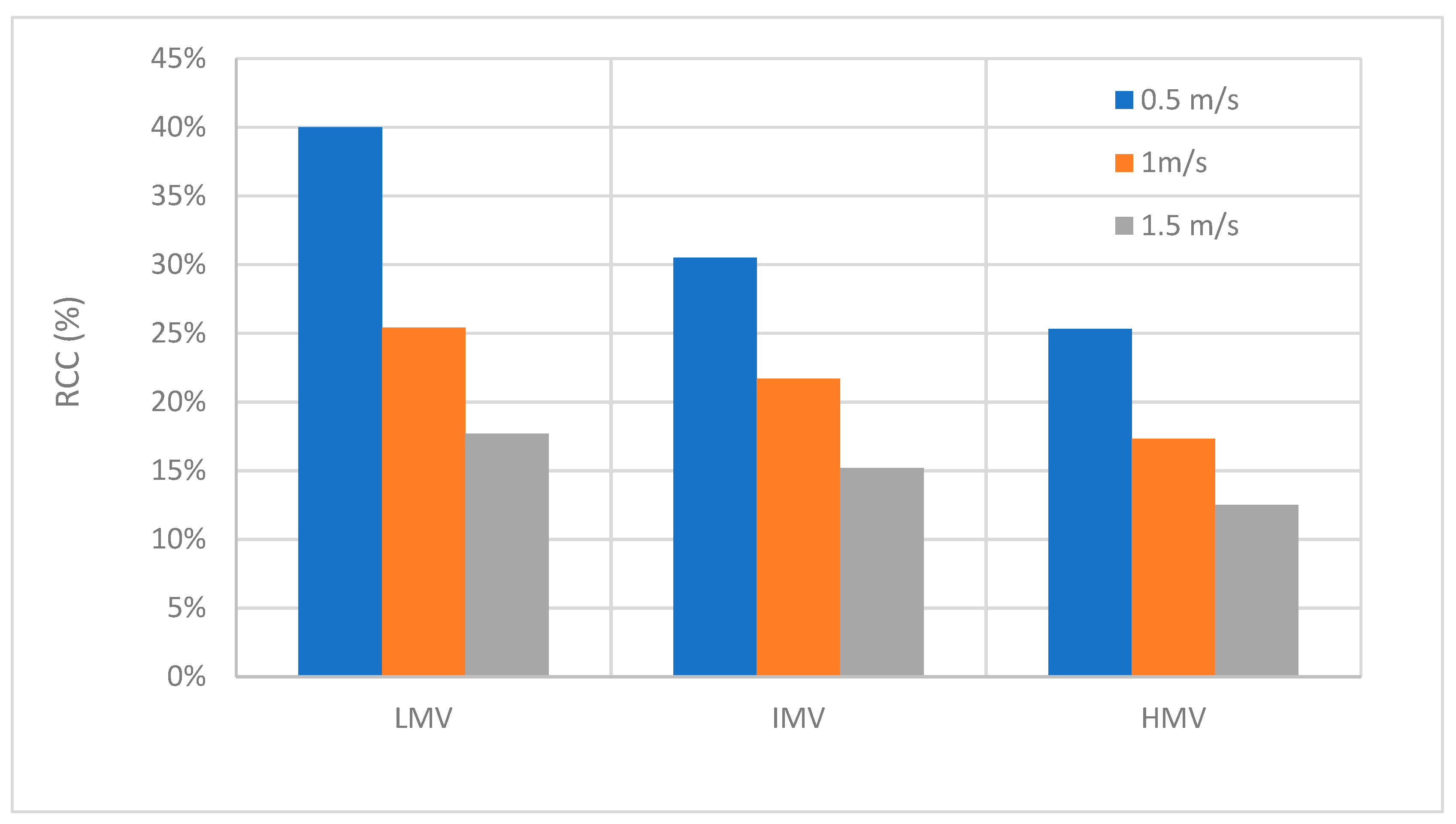
3.1. Effects of Mud Rheology

The effect of mud rheology on the RCC at different annular velocities for the horizontal annulus is presented in Figure 7. In these series of simulations, the cutting size was 1.4 mm, and the drill pipe rotated at 60 rpm. As shown, increasing the mud viscosity from LMV to HMV resulted in a decrease in RCC and an increase in cleaning efficiency in the annulus at all ranges of velocities. By changing from low-viscosity mud (LVM) to HVM at constant velocities of 0.5 m/s, 1 m/s, and 1.5 m/s, RCC decreases by 38%, 32%, and 30%, respectively. It can be derived that the impact of rheology on the cuttings transport is less at higher flow rates.
The effects of mud viscosity on the cleaning efficiency at different inclination angles for different mud velocities are presented in Figure 8, Figure 9 and Figure 10. In this series of simulations, cutting size was 1.4 mm and drill pipe rerated at 60 rpm. Simulations were carried out for 0.5, 1, and 1.5 m/s mud velocities. The results in Figure 8 and Figure 9 show that at 1.5 m/s and 1 m/s mud velocities, the RCC rises with an increase in the angle of inclination (from vertical to horizontal) for all types of mud. However, at 1.5 m/s mud velocity, increasing the mud viscosity from LMV to HMV reduces the RCC by 35%, 30%, and 8% for 45-degree horizontal and vertical annulus, respectively, suggesting that the effect of mud viscosity on RCC reduction is more pronounced for the 45 degree-inclined annulus. The same trend can be observed for 1 m/s mud velocity.
However, as shown in Figure 10 for all mud viscosities, at 0.5 m/s mud velocity, RCC increases as the well is deviated from vertical to 45 degrees, while it drops when the angle is further changed from 45 degrees to horizontal. Figure 11 shows the snapshots of cutting distribution in the annulus for different inclinations at 0.5 m/s mud velocity. Qualitatively, it can be seen that at 0.5 m/s mud velocity there are fewer cuttings, with a more uniform distribution for the vertical well as compared to the inclined wells. For the horizontal well, there are higher accumulations of cuttings near the bottom wall due to gravity. Nevertheless, at this annular velocity, the 45-degree well will have the highest RCC, as quantitatively shown in Figure 10. It is worth pointing out that Tomren et al. [2] also reported that the cuttings concentration faced an increase at inclination angles near 45 ° at lower annular velocities (@0.59 m/s) [2], though in their study, the particle concentration is significantly higher than in this work. This could be caused by the cuttings sliding down along the lower wall of the annulus, which nullifies the impact of other parameters.

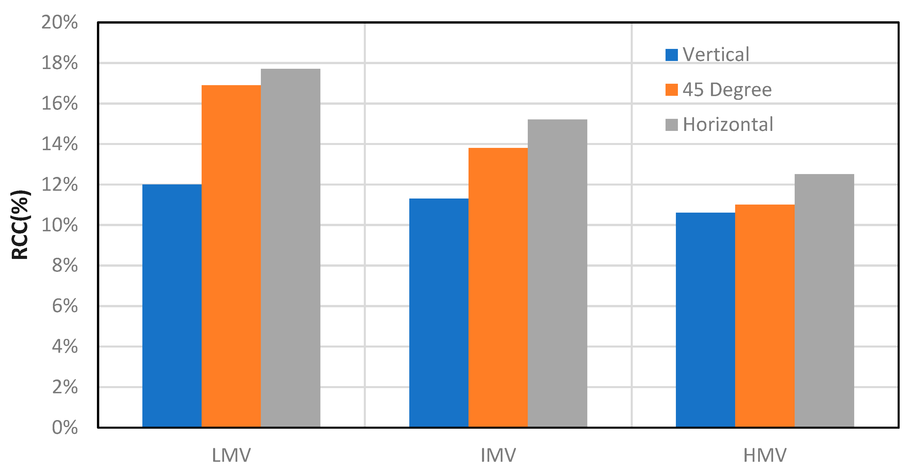
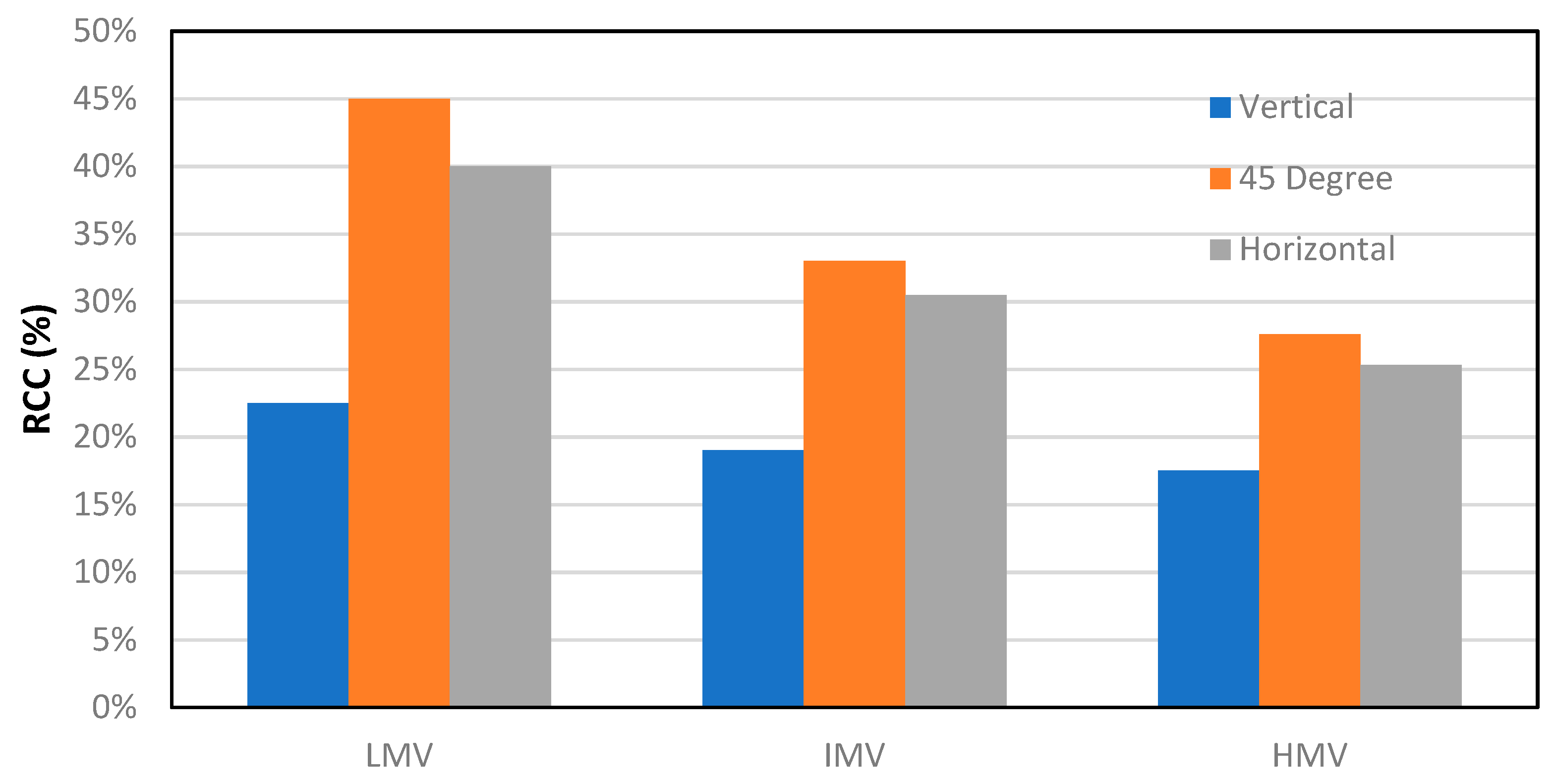
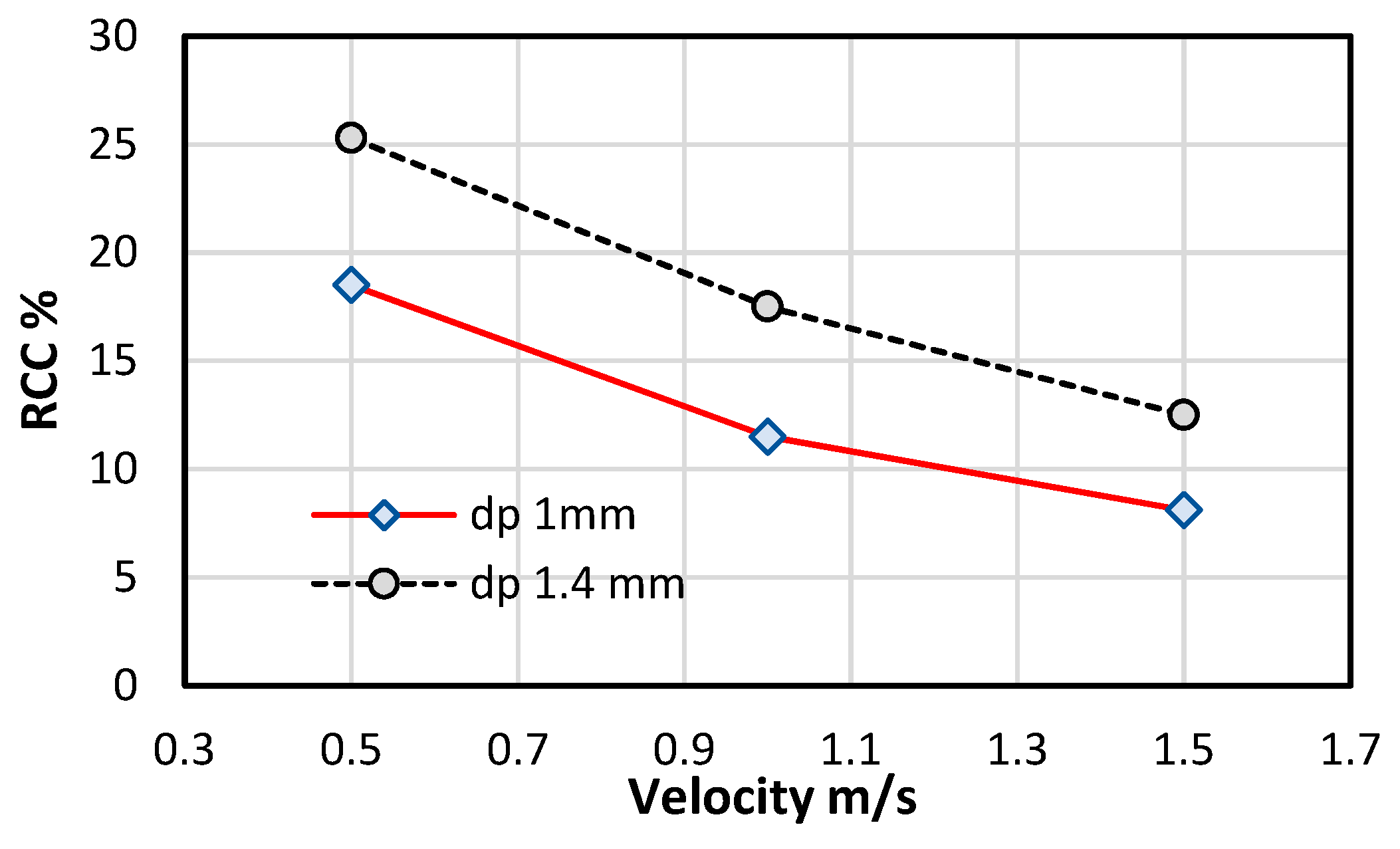
3.2. Effect of Cuttings Size on RCC

The effect of particle size on RCC is studied for the average particle diameters of 1 mm and 1.4 mm. In these series of simulations, annular velocities varied from 0.5 to 1.5 m/s, but the mud viscosity was kept constant (HVM). The inner pipe was rotated at 60 rpm. Simulation results of RCC versus mud velocity for two different particle sizes are illustrated in Figure 12. It can be seen that by reducing the cutting size from 1.4 mm to 1 mm at velocities of 0.5, 1, and 1.5 m/s, the RCC reduces by 27%, 34%, and 35%, respectively. According to Equations (12) and (13), the slip velocity and Stokes number are lower for smaller particles. Consequently, small particles are more easily removed from the annulus. By increasing the annular velocity from 0.5 to 1.5 m/s, the RCC reduces by 50% for larger particles, while it reduces by 57% for the smaller cutting sizes, suggesting that the impact of mud velocity on RCC is slightly less pronounced for larger particles.

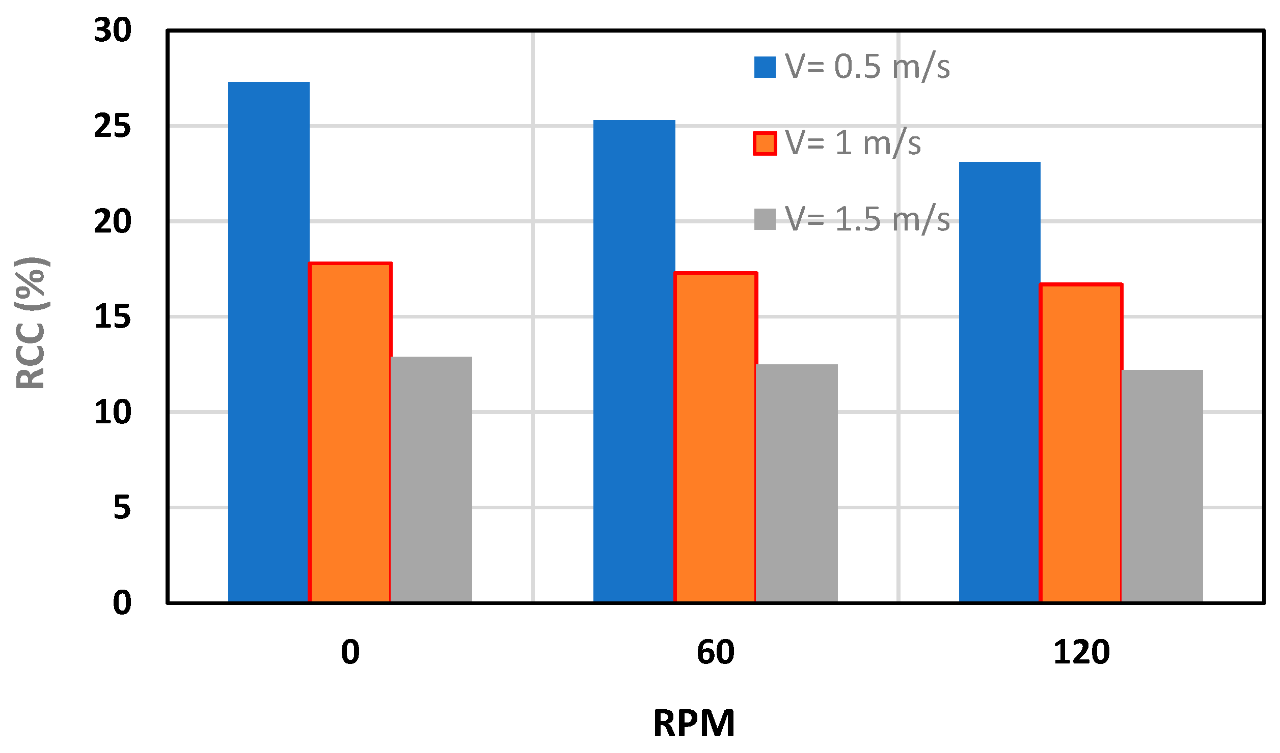
3.3. Effect of Drill Pipe Rotation

The effect of drill pipe rotation on RCC for various mud velocities is investigated in this section. Simulations were carried out with an average particle size of 1.4 mm and constant mud viscosity (HVM), but with varying annular velocities, as shown in Figure 13. It is observed that an increase in the drill pipe rotation tends to slightly reduce the RCC in the annulus; i.e., by increasing the drill pipe rotation from zero to 120 RPM at 0.5, 1, and 1.5 m/s mud velocities, RCC reduces by 15%, 7%, and 5%, respectively. Increasing the drill pipe rotation motivates the cuttings to travel in the middle of the annulus rather than near the walls due to the lifting effect. Moreover, it can be observed that at higher mud velocities, the impact of drill pipe rotation on cuttings concentration in the annulus is lower, and the drill pipe rotation yields negligible improvement in the cuttings transport rate in the annulus. In comparison with other parameters investigated in this study, drill pipe rotation shows less impact on cleaning efficiency under turbulent flow regime, and it is more pronounced at lower annular velocities.
The snapshot of particle dispersion is framed in Figure 14, where the effect of drill pipe rotation can be seen for 0.5 m/s.

3.4. Discussion

The parametric study in this work implies that different factors can reduce the RCC and improve the hole cleaning. For deviated wells, increasing mud viscosity has significant impact on the hole cleaning, while for vertical wells, mud velocity has a more pronounced effect on the hole cleaning. This could be due to the domination of the axial component of particles’ slip velocity in vertical wells and the drag effects, as compared to the behavior of particles in deviated wells. However, in practice, there are limitations on the level of mud viscosity and pumping rate (mud velocity). An increase in mud viscosity can lead to a higher pressure drop in the annulus, requiring higher pumping power and surface pressure for mud circulation. While this will increase the equivalent circulation density (ECD) of the mud, the surface pressure can approach the maximum allowable annular surface pressure (MAASP), beyond which an unwanted formation fracture can occur. Hence, the drilling engineers should optimize the mud viscosity and pumping rate with the consideration of pressure drop and MAASP.
On the other hand, in highly deviated and horizontal drillings a rotary steerable drilling system (RSS) is normally used, which enables drilling without the rotation of the pipe. The current study implies that lack of drill pipe rotation may have minimal effect on the cutting transport if a sufficient mud-pumping rate (mud velocity) is used.
Moreover, our study shows that RCC increases with the particle size, leading to a lower hole cleaning efficiency for larger particles. However, RCC can be reduced if higher mud velocities are used. Hence, one can conclude that for the optimization of hole cleaning, the drilling engineers should design the mud properties and its pumping rate (mud velocity) according to the larger cuts of particles, while considering safe and operable conditions of the mud circulation, as stated earlier.
This study has provided an insight into the effect of mud rheology and drilling conditions on the efficiency of cutting transport using unresolved DEM–CFD simulations and spherical particles; however, as there will be improvements in the computational power and simulation algorithm, future work could be extended to the simulation of penetration of drill bit into the formation, as a result of which, particles of different shapes and sizes could be produced.

4. Conclusions

In this study, a fully coupled CFD–DEM model is simulated to study the effect of the mud rheology, cutting size, well inclination, and drill pipe rotation on the hole-cleaning process, where the relative cuttings concentration (RCC) is defined to represent the cuttings transport performance in the annulus. In terms of the effects of mud rheology on cuttings transport, where the mud behavior obeys the Herschel–Buckley viscosity model, three types of mud viscosity (high, intermediate, and low) have been examined in the CFD–DEM model. In this work, mud velocities varied from 0.5 m/s to 1.5 m/s for vertical, 45-degree, and horizontal wells, while the drill pipe rotation was changed from 0 to 120 rpm.
In conclusion, the main findings of this study can be summarized as follows:
  • Mud annular velocity has a dominant effect on RCC. Lower RCC and better cleaning performance can be achieved by increasing mud velocity to its limiting value for all ranges of well inclinations.
  • At all well inclination angles, the RCC is lowest at high mud viscosity; however, the effect of mud viscosity is more pronounced at lower annular mud velocities. By increasing the velocity, the impact of mud viscosity on RCC is reduced.
  • RCC increases from vertical to horizontal wells at higher mud velocities, but at low mud velocity (0.5 m/s), the 45-degree well has the highest RCC.
  • The impact of drill pipe rotation is more pronounced for lower values of annular mud velocity. Increasing drill pipe rotation from zero to 120 rpm improves the cleaning efficiency in deviated annuli at lower velocities, while it has very little effect for the vertical annulus.

Author Contributions

Conceptualization, A.Z. and A.H.; Methodology, A.Z. and M.A.B.; Formal analysis, A.Z.; Investigation, A.Z. and A.H.; Writing—original draft, A.Z.; Writing—review & editing, M.A.B. and A.H.; Supervision, M.A.B. and A.H. All authors have read and agreed to the published version of the manuscript.

Funding

This research was funded by the EPSRC for the project funding (EP/N509681/1) and support at the University of Leeds.

Data Availability Statement

The data presented in this study are available on request from the corresponding author.

Conflicts of Interest

The authors declare no conflicts of interest.

References

  1. Zeidler, U.H. An experimental analysis of the transport of drilled particles. Soc. Pet. Eng. J. 1972, 12, 39–48. [Google Scholar] [CrossRef]
  2. Tomren, P.H.; Lyoho, A.W.; Azar, J.J. Experimental study of cuttings transport in directional wells. SPE Drill. Eng. 1986, 1, 43–56. [Google Scholar] [CrossRef]
  3. Brown, N.P.; Bern, P.A.; Weaver, A. Cleaning deviated holes: New experimental and theoretical studies. In Proceedings of the SPE/IADC Drilling Conference, New Orleans, LA, USA, 28 February–3 March 1989. [Google Scholar]
  4. Peden, J.M.; Ford, J.A.; Oyeneyin, M.B. Comprehensive experimental investigation of drilled cuttings transport in inclined wells including the effects of rotation and eccentricity. In Proceedings of the European Petroleum Conference, The Hague, The Netherlands, 21–24 October 1990. [Google Scholar]
  5. Sifferman, T.R.; Becker, T.E. Hole cleaning in full-scale inclined wellbores. SPE Drill. Eng. 1992, 7, 115–120. [Google Scholar] [CrossRef]
  6. Bassal, A.A. The Effect of Drillpipe Rotation on Cuttings Transport in Inclined Wellbores. Ph.D. Thesis, University of Tulsa, Tulsa, OK, USA, 1995. [Google Scholar]
  7. Sanchez, R.A.; Azar, J.J.; Bassal, A.A.; Martins, A.L. The effect of drillpipe rotation on hole cleaning during directional well drilling. In Proceedings of the SPE/IADC Drilling Conference, Amsterdam, The Netherlands, 4–6 March 1997. [Google Scholar]
  8. Yu, M.; Takach, N.E.; Nakamura, D.R.; Shariff, M.M. An experimental study of hole cleaning under simulated downhole conditions. In Proceedings of the SPE Annual Technical Conference and Exhibition, Anaheim, CA, USA, 11–14 November 2007. [Google Scholar]
  9. Bilgesu, H.I.; Ali, M.W.; Aminian, K.; Ameri, S. Computational Fluid Dynamics (CFD) as a tool to study cutting transport in wellbores. In Proceedings of the SPE Eastern Regional Meeting, Lexington, KY, USA, 23–26 October 2002. [Google Scholar]
  10. Bilgesu, H.I.; Mishra, N.; Ameri, S. Understanding the effect of drilling parameters on hole cleaning in horizontal and deviated wellbores using computational fluid dynamics. In Proceedings of the Eastern Regional Meeting, Lexington, KY, USA, 17–19 October 2007. [Google Scholar]
  11. Wang, Z.-M.; Guo, X.-L.; Li, M.; Hong, Y.-K. Effect of drillpipe rotation on borehole cleaning for extended reach well. J. Hydrodyn. 2009, 21, 366–372. [Google Scholar] [CrossRef]
  12. Yilmaz, D. Discrete Phase Simulations of Drilled Cuttings Transport Process in Highly Deviated Wells. Master’s Thesis, Louisiana State University, Baton Rouge, LA, USA, 2013. [Google Scholar]
  13. Rooki, R.; Ardejani, F.D.; Moradzadeh, A.; Norouzi, M. Simulation of cuttings transport with foam in deviated wellbores using computational fluid dynamics. J. Pet. Explor. Prod. Technol. 2014, 4, 263–273. [Google Scholar] [CrossRef]
  14. Mohammadzadeh, K.; Hashemabadi, S.; Akbari, S. CFD simulation of viscosity modifier effect on cutting transport by oil based drilling fluid in wellbore. J. Nat. Gas Sci. Eng. 2016, 29, 355–364. [Google Scholar] [CrossRef]
  15. Amanna, B.; Movaghar, M.R.K. Cuttings transport behavior in directional drilling using computational fluid dynamics (CFD). J. Nat. Gas Sci. Eng. 2016, 34, 670–679. [Google Scholar] [CrossRef]
  16. Tong, T.; Ozbayoglu, E.; Liu, Y. A Transient Solids Transport Model for Solids Removal Evaluation in Coiled-Tubing Drilling. SPE J. 2021, 26, 2498–2515. [Google Scholar] [CrossRef]
  17. Akhshik, S.; Behzad, M.; Rajabi, M. CFD–DEM approach to investigate the effect of drill pipe rotation on cuttings transport behavior. J. Pet. Sci. Eng. 2015, 127, 229–244. [Google Scholar] [CrossRef]
  18. Akhshik, S.; Behzad, M.; Rajabi, M. CFD-DEM simulation of the hole cleaning process in a deviated well drilling: The effects of particle shape. Particuology 2016, 25, 72–82. [Google Scholar] [CrossRef]
  19. Akhshik, S.; Behzad, M.; Rajabi, M. On the particle–particle contact effects on the hole cleaning process via a CFD–DEM model. Part. Sci. Technol. 2016, 34, 736–743. [Google Scholar] [CrossRef]
  20. Akhshik, S.; Rajabi, M. CFD-DEM modeling of cuttings transport in underbalanced drilling considering aerated mud effects and downhole conditions. J. Pet. Sci. Eng. 2018, 160, 229–246. [Google Scholar] [CrossRef]
  21. FLUENT Inc. Chapter 10. Modeling Turbulence; FLUENT Inc.: Lebanon, NH, USA, 2001; pp. 1–102. [Google Scholar]
  22. Saasen, A.; Ytrehus, J.D. Viscosity Models for Drilling Fluids—Herschel-Bulkley Parameters and Their Use. Energies 2020, 13, 5271. [Google Scholar] [CrossRef]
  23. Sommerfeld, M. Theoretical and experimental modelling of particulate flows. Lect. Ser. 2000, 6, 3–7. [Google Scholar]
  24. Kuang, S.B.; Yu, A.B.; Zou, Z.S. Computational study of flow regimes in vertical pneumatic conveying. Ind. Eng. Chem. Res. 2009, 48, 6846–6858. [Google Scholar] [CrossRef]
  25. Rowe, P.N. Drag forces in a hydraulic model of a fluidized bed-part I. Trans. Inst. Chem. Eng. 1961, 39, 43–54. [Google Scholar]
  26. Zeidler, H.U. An experimental analysis of the transport of drilled particles in an annulus. J. Pet. Technol. 1970, 22, 1055. [Google Scholar]
  27. Schetz, J.A.; Fuhs, A.E. Fundamentals of Fluid Mechanics; John Wiley & Sons: Hoboken, NJ, USA, 1999. [Google Scholar]
  28. Sifferman, T.R.; Myers, G.M.; Haden, E.L.; Wahl, H.A. Drill cutting transport in full scale vertical annuli. J. Pet. Technol. 1974, 26, 1295–1302. [Google Scholar] [CrossRef]
  29. Okrajni, S.; Azar, J.J. The effects of mud rheology on annular hole cleaning in directional wells. SPE Drill. Eng. 1986, 1, 297–308. [Google Scholar] [CrossRef]
Figure 1. Annular velocity > cuttings slip velocity.
Processes 12 00784 g001
Figure 2. Computational diagram of the CFD–DEM framework.
Processes 12 00784 g002
Figure 3. Geometry domain and boundary conditions.
Processes 12 00784 g003
Figure 4. Mesh independency study; vertical annulus, mud annular velocity of 1.5 m/s.
Processes 12 00784 g004
Figure 5. Computational grid on the cross section of the concentric annulus. Rin and Rout are inner and outer radii, respectively.
Processes 12 00784 g005
Figure 6. Number of particles remaining in the annulus in a horizontal wellbore, 1.5 m/s, 60 rpm, dp = 1.4 mm, HVM.
Processes 12 00784 g006
Figure 7. Effect of mud rheology on RCC at different flow velocities; horizontal annulus, (dp = 1.4 mm).
Processes 12 00784 g007
Figure 8. Effect of rheology on RCC at different angles of inclination (velocity 1.5 m/s).
Processes 12 00784 g008
Figure 9. Effect of rheology on RCC at different angles of inclination (velocity 1 m/s).
Processes 12 00784 g009
Figure 10. Effect of rheology on RCC at different angles of inclination (velocity 0.5 m/s).
Processes 12 00784 g010
Figure 11. Effects of inclination on cuttings transport mechanism at annular velocity of 0.5 m/s.
Processes 12 00784 g011
Figure 12. Effect of cuttings size on cleaning efficiency at different mud velocities (60 rpm and HMV).
Processes 12 00784 g012
Figure 13. Effect of inner pipe rotation on cuttings concentration in horizontal annulus.
Processes 12 00784 g013
Figure 14. Effect of drill pipe rotation in cuttings trajectory in horizontal annulus at V = 0.5 m/s.
Processes 12 00784 g014
Table 1. Simulation input parameter.
ParameterExperimental Work of Tomren et al. (1986) [2]Simulation Data in This WorkUnits
Drill string length121.5m
Angle of inclination0, 20, 40, 60, 800, 45, 90deg
Wellbore (hole) diameter 127120 (4.75′′)mm
Drill pipe diameter48.2650mm
Drill pipe rotation (rpm)0, 5060, 120rpm
Eccentricity ratio0.50-
Fluid behaviour index (n)0.650.65-
Consistency index (k)0.280.28Pa.sn
Fluid inlet velocity0.58, 0.72, 0.87, 1.10.5, 1, 1.5m/s
Fluid density10181018Kg/m3
Particle density26192600Kg/m3
Particle shear modulus 10MPa
Particle coefficient of restitution 0.5-
Particle coefficient of sliding friction 0.5-
Particle coefficient of rolling friction 0.05-
Cutting diameter (average)6.350.8–1.1 (1), 1.3–1.5 (1.4)mm
Table 2. Rheological Properties of Mud Fluid Studied.
Drilling FluidLow-Viscosity Mud (LVM)Intermediate-Viscosity Mud (IVM)High-Viscosity Mud (HVM)
Apparent Viscosity (Pa·s)0.0040.0130.028
Plastic Viscosity (Pa·s)0.0030.0090.019
Yield Point (Pa)0.548
Mud Re9000–26,0003000–80004000–12,000
Particle Re1 < 89–143 < 10001 < 13–18 < 10001 < 3–6 < 1000
Slip Velocity (m/s)0.25–0.40.12–0.160.05–0.12
Particle Stokes Number1–1.50.15–0.450.07–0.2
Disclaimer/Publisher’s Note: The statements, opinions and data contained in all publications are solely those of the individual author(s) and contributor(s) and not of MDPI and/or the editor(s). MDPI and/or the editor(s) disclaim responsibility for any injury to people or property resulting from any ideas, methods, instructions or products referred to in the content.

