Optimizing Accumulator Performance in Hydraulic Systems through Support Vector Regression and Rotational Factors

Abstract

The piston-type accumulator is an energy storage device in hydraulic–pneumatic systems, playing a significant role in industries such as petrochemicals, heavy machinery, and steel metallurgy. The displacement parameters of the piston-type accumulator are vitally important for fault diagnosis and early warning in hydraulic systems. Traditional displacement measurement methods cannot meet the requirements of the internal testing environment of the accumulator. Therefore, this paper proposes an accumulator piston displacement signal compensation method based on rotational factors and support vector regression. Firstly, empirical mode decomposition is utilized to denoise the signal. Then, rotational factors are used to generate a delay compensation module to compensate for the signal attenuation and time delay caused by metallic reflection and scattering within the cylinder of the radar signal. The support vector regression model is improved based on a hash table to enhance its computational efficiency and achieve radar displacement signal compensation. Finally, a simulation experiment is designed to verify the effectiveness of the proposed method.

1. Introduction

Piston accumulators serve as energy storage devices in hydraulic pneumatic systems and play an important role in industries such as petrochemicals, large machinery, and steel metallurgy. The structure of the mainstream piston accumulator is shown in Figure 1, with the part names corresponding to the numbers in Figure 1, as shown in

Table 1. Piston Accumulator Assembly Parts List.

Serial Number	Component
1	Oil Port End Cap
2	Type O ring $\varphi$ 170 $\times 5.3$
3	Retaining ring $\varphi 180\times \varphi 172\times 5.3$
4	cylinder liner
5	piston
6	guide belt
7	Gram circle $\varphi 159\times \varphi 180\times 8.1$
8	End cap of air nozzle
9	Check valve
10	washer
11	Inflatable valve assembly end cap
12	protector
13	Bolt M8$\times 16$
14	Gram circle $\varphi 159\times \varphi 180\times 8.1$

.

The external container of a piston accumulator is usually a cylindrical metal casing. This casing is used to enclose the stored fluid while also protecting the internal components from the external environment. The piston is a movable part that seals tightly with the inner wall of the casing. It can move within the casing, changing the internal volume based on the compression or expansion of the fluid. The energy storage and release process of the piston accumulator are both related to the movement of the piston. Piston accumulators use seals to keep the fluid from leaking inside the casing. These seals are usually located at the contact surface between the piston and the casing to prevent fluid leakage. Piston accumulators mainly have two working processes, including the energy storage process and the energy release process. When the external hydraulic system applies pressure to push fluid into the accumulator, the piston moves under the pressure, reducing the internal volume. This causes the fluid to be compressed in the space between the piston and the casing, thereby storing energy. This process is similar to compressing a spring. When the system needs to release the stored energy, the piston of the accumulator is forced to move outward, increasing the internal volume. This allows the stored compressed fluid to flow back into the system, providing additional hydraulic energy.

Because piston accumulators are mainly used in hydraulic systems, the piston displacement parameters within the piston accumulator tank are very important for fault diagnosis and early warning in hydraulic systems [1]. Accurate detection of displacement parameters is of significant importance for enterprise safety production. Common level displacement detection devices include buoyancy-type, piezoelectric sensor-type, ultrasonic echo-type [2], waveguide-type, and laser infrared-type [3,4]. The buoyancy-type detection device has a simple principle and structure, reducing the chances of failure, and is easy to maintain, but it is not suitable for high-viscosity liquids in practical use. The capacitive-type has low installation requirements, is adaptable to various environments, and is unaffected by the properties of the liquid, but may produce false readings with adhering conductive liquids. The waveguide-type can achieve non-contact measurement with long-term stability, but it is challenging to maintain where tight sealing is required. Optical sensors provide high detection precision and are unaffected by the electrical characteristics of the medium; however, they cannot penetrate in dusty and smoky environments and their use is limited in liquid media detection. Radar sensors are highly accurate and can adapt to extreme conditions, featuring non-contact measurement, making them suitable for the detection environment of high-viscosity and corrosive liquids, and are the preferred choice in industries such as chemical smelting [5,6].

The error in detecting piston displacement with a radar sensor can stem from several factors, including reflections off the metallic cylinder, measurement distance, and angle limitations. The cylinder of an accumulator is typically made of metal and, when radar signals are emitted, the metal can efficiently reflect the radar waves, resulting in echo signals that arrive at the receiver via different paths. Although these signals all originate from the reflective antenna, the paths they travel are varied, and their transit times differ. When these signals are added together at the receiver, their phase inconsistency leads to waveform broadening, distortion, and multipath effects [7], adversely affecting signal quality [8]. This can cause anomalies in the radar waveform and increase measurement errors. Furthermore, the precision of a radar sensor is somewhat dependent on the distance to the target; at close range, radar waves may produce strong echoes, complicating signal processing and affecting measurement accuracy. If the piston’s surface is not perfectly perpendicular to the sensor, meaning the radar wave’s angle of incidence is not 90°, this can cause the radar waves to reflect at angles different from what is expected, resulting in measurement errors. The errors caused by the aforementioned reasons present complex nonlinear characteristics, making them difficult to compensate for quantitatively.

2. Related Works

Currently, compensation methods for output signals primarily include traditional signal processing compensation and signal compensation techniques that incorporate machine learning algorithms. Traditional signal compensation employs Kalman filters [9] to predict and correct signals processed based on time series analysis, thereby achieving signal compensation. Traditional signal processing methods are sensitive to noise and outliers, resulting in poor adaptability for dealing with nonlinear and non-stationary signals. Signal compensation methods that incorporate machine learning algorithms mainly achieve feature extraction through the preprocessing of original signals, select appropriate machine learning algorithms, optimize algorithm adjustments for model parameters, and complete signal compensation. Reference [10] proposed minimizing the entropy corresponding to the echo signals as the objective function and using the Particle Swarm Optimization (PSO) algorithm to search for global optimum parameters to achieve compensation of joint motion signals. Reference [11] introduced a dynamic compensation feature in the Regularized Generalized Orthogonal Matching Pursuit algorithm, which identifies and suppresses resonant noise based on the signal’s priori features and directly reconstructs denoised signals from subsampled measurements of the original signal. Reference [12] presented a signal compensation method that combines the Sparse Fast Fourier Transform (SFFT) and the Iterative Adaptive Approach (IAA). Reference [13] offered a roller eccentricity signal compensation method based on improved Particle Swarm Optimization and wavelet threshold denoising. The method applies wavelet denoising to signals and uses eccentricity compensated signals in the automatic thickness control system of cold rolling mills. Reference [14] introduced a phase compensation method that aligns the phases of all signals and weights the average of all pulse response signals to eliminate random noise. Reference [15] proposes a novel two-dimensional autofocusing algorithm for airborne strip map THz-SAR imaging for practical applications. It simultaneously estimates amplitude and phase errors in the range frequency domain based on dominant point targets selected in the preliminarily focused image. Reference [16] proposes the use of the linear Doppler effect to detect the translational motion of objects and provides a detailed description of the properties and analysis methods of rotational Doppler shift when the vortex beams are misaligned with the rotation axis.

References [10,11] both proposed methods based on parameterized compensation and calibration; however, since radar measurement of accumulator piston displacement usually occurs in a high signal-to-noise ratio environment, this makes compensation challenging. References [12,13] both employed feature extraction methods to extract characteristics, such as frequency, amplitude, and phase, from rolling eccentricity signals, but rolling eccentricity signals and accumulator piston displacement signals differ in source, characteristics, and application scenarios. References [14,15] aimed to eliminate distortions caused by signal nonlinearity or phase delays, but real-time acquisition and processing of displacement signal data for accumulator piston displacement are subject to time delays or computational load restrictions. Reference [16] proposed methods for dealing with signal distortion caused by unstable environments, but the distortion of accumulator piston displacement arises from a mix of various environmental factors.

To address the above issues, while also requiring simple hardware implementation, fast processing speed, and ease of engineering application, this paper proposes a method for compensating the displacement signal of accumulator pistons. Firstly, the Empirical Mode Decomposition (EMD) [17] is utilized for preliminary signal denoising, then a rotational factor is used to generate a delay compensation module to compensate for signal attenuation and time delays caused by metal reflections, measurement distance, and angle limitations. Improved SVR models [18] are employed for radar displacement signal compensation. Finally, cylinder simulation experiments are conducted for experimental verification.

3. Principle of FMCW Radar Range Measurement

The full name of FMCW radar is Frequency-Modulated Continuous-Wave radar. It operates by continuously transmitting a signal whose frequency varies over time, and then receiving the signal reflected back from the target. By analyzing the frequency difference between the transmitted and received signals, the radar can measure parameters such as the distance and speed of the target.

The structure of the FMCW radar system [19] is shown in Figure 2, which is divided into five main parts: frequency source, transceiver branch, transceiver antenna, signal processing, and result display. The transceiver branch mainly consists of a power divider, mixer, and low-noise amplifier (LNA), which are responsible for the up-conversion and down-conversion processing of the transmitted and received signals. The LNA, in particular, has a relatively low noise figure; it selectively amplifies the echo signal and, by suppressing noise signals, relatively increases the system sensitivity and signal-to-noise ratio (SNR). The transceiver antenna can be chosen according to the specific application scenario. The use of transmit/receive isolation eliminates the need for devices such as circulators, achieving higher isolation; the signal processing section mainly performs both analog and digital signal processing tasks.

For the measurement of targets, the frequency-modulated continuous wave (FMCW) radar’s frequency modulation curves for the transmitted and echo signals are shown in Figure 3. The red line represents the transmitted signal, while the green line represents the echo signal. By taking the beat frequency of the transmitted and echo signals, the intermediate frequency (IF) signal can be obtained. Based on the signal propagation delay time between the transmitted and echo signals, multiplying it by the speed of light provides the distance information for the target. as shown in Figure 4.

If the target distance is denoted as $R$, and the speed of light is represented by $c$, then the time delay of the echo signal is given by:

$$\tau =\frac{2R}{c}$$

(1)

where $\tau$ represents the time delay between the transmitted signal and the echo signal. The target distance is given by:

$$R=\frac{Tc}{4B}{f}_{IF}$$

(2)

where $f_{IF}$ represents the frequency value of the intermediate frequency signal, $B$ represents the bandwidth, which is the range of frequency modulation in the radar’s transmitted signal, and $T$ is the period of a complete cycle.

In the FMCW radar system, when the radar signal intersects with strong reflective surfaces, such as metal, multipath effects occur. Taking into account multipath effects, there may be multiple reflection points at different positions in the signal propagation path. Therefore, for a reflection point, the introduced time delay ${\tau }_i$ and the corresponding intermediate frequency signal $f_{IFi}$ can be expressed as:

$${\tau }_i=\frac{2R_i}{c}$$

(3)

$$f_{IFi}=\frac{4B{R}_i}{Tc}$$

(4)

where $R_i$ is the virtual distance corresponding to the $i$ reflection path. Therefore, the total intermediate frequency signal $f_{IFtotal}$ under multipath effects can be expressed as the summation of the frequency signals from all valid reflection paths:

$$f_{IFtotal}={\displaystyle \sum f_{IFi}}$$

(5)

The difference between $f_{IFtotal}$ caused by multipath effects and the ideal single-path $f_{IF}$ can lead to errors in estimating the target distance. Particularly when the delays of multiple paths are similar, their signals will overlap in the spectrum, making it difficult for the radar to distinguish between signals corresponding to the direct path and those corresponding to reflected paths.

When multiple reflection points are in close proximity to each other, the reflected signals they produce will overlap in terms of time delay. Processing time-delayed signals can differentiate these closely situated targets. Identifying which signals are generated by the direct path and which are the result of multipath reflections enables signal compensation under metallic reflection conditions.

4. Compensation Method for Accumulator Piston Displacement Signal

The compensation method for accumulator piston displacement signals is divided into three main stages: EMD signal denoising and reconstruction, processing and improvement of the delay compensation module based on rotation factor, and compensation with SVR model improvement.

Firstly, denoising and reconstruction are achieved based on EMD; echo signals are processed with matched filtering to eliminate Doppler effects, increase gain factors, and reduce the impact of signal attenuation on subsequent compensation effects. An improved cross-correlation method for calculating signal fundamental frequency is employed by applying a signal-to-noise ratio threshold. Rotation factors are fitted using the least squares method, and delay compensation signals are calculated in combination with time correction. Finally, a dual hash table is constructed to improve parameter grid search, and accumulator piston displacement signal compensation is implemented based on support vector regression (SVR).

4.1. EMD Decomposition Achieves Signal Denoising

Due to the presence of nonlinear and non-stationary characteristics, such as mechanical vibration, fluid dynamics, and oil variations in the displacement signals measured inside the cylinder, the EMD method can adapt to these variations and extract the real signal components, enabling better identification and analysis of the dynamic behavior of the signal. The noise after EMD decomposition is a normally distributed signal, and each Intrinsic Mode Function (IMF) corresponds to only one frequency value at each moment. In other words, IMF is a single-component signal. Based on this characteristic, the different frequency components of the noise signal can be decomposed into different IMF components.

Calculate the relative power increase factor RPi as follows. Calculate the product of energy density and mean period for the first IMF component, denoted as E1. Since this is the first IMF component without a preceding IMF component, RPi1 = 0. For each subsequent IMF component (starting from the second IMF component), calculate the product of energy density and mean period, denoted as Ei. Calculate RPi using the following formula:

Calculate RPi using the following formula:

$$RPi=Ei/E(i-1)$$

(6)

where i represents the index of the current IMF component. When the value of RPi is greater than or equal to 1, it indicates a significant increase in the product of energy density and mean period of the current IMF component relative to the preceding IMF component.

Filtering IMF components: When the value of RPi is greater than or equal to 1, it is considered that the preceding IMF components mainly contain noise, and therefore they are removed. Then, the remaining IMF components are used to reconstruct the signal in order to achieve denoising of the original noisy signal.

4.2. Generate Delay Compensation Module Based on Rotation Factor

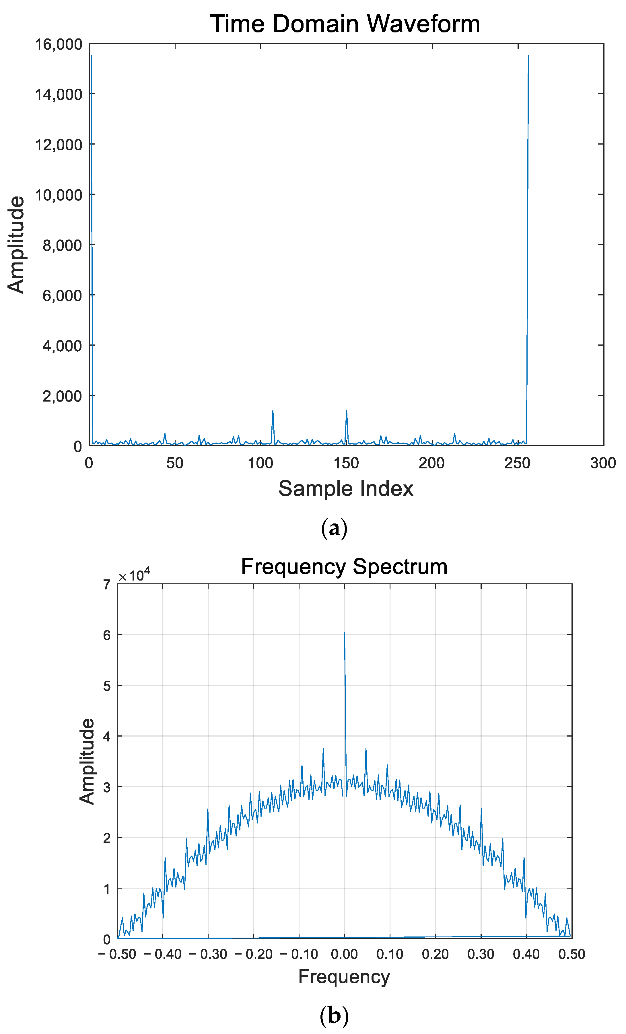
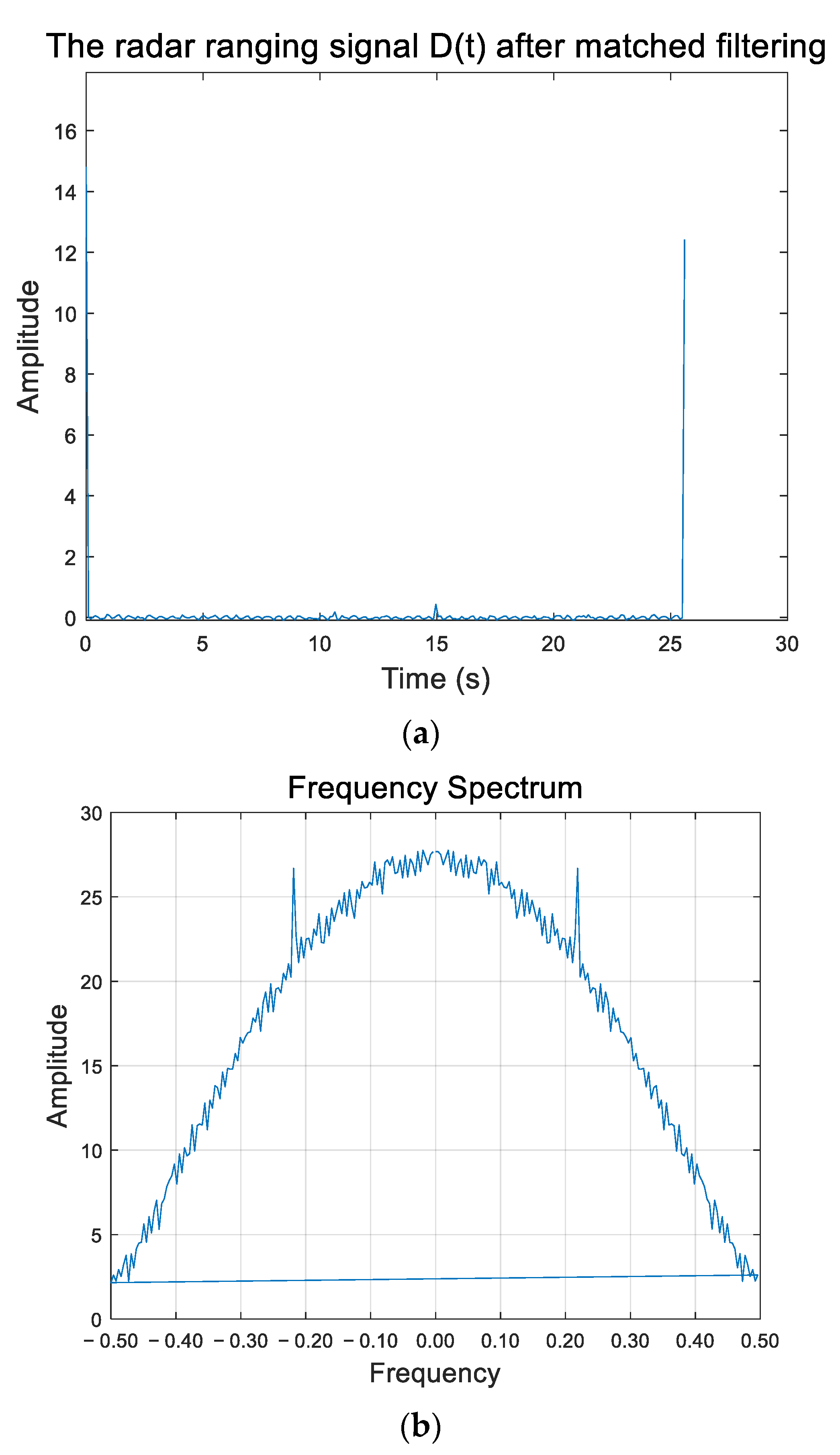
4.2.1. Matched Filter Gain Algorithm

For the measurement of distance and angle restrictions, the length of the piston accumulator generally does not exceed 2 m, while the maximum range of the experimental system used is 3 m. In addition, when the piston moves vertically to the cylinder, radar measurements do not have angle restrictions. Therefore, the error in radar sensor detection of piston displacement mainly comes from the metal reflection of the accumulator cylinder. Since the piston of the accumulator is a metal product, the radar measurement echo signal contains scattered and reflected interference signals, causing their frequency components to mutually superimpose with the Doppler frequency shift of the target. In this case, it becomes quite difficult to accurately extract precise distance information related to the piston displacement.

The design of the matched filter is specific to the signal shape emitted by the radar system. When the radar receiver receives interference signals generated by internal or external objects in the system, the filter suppresses these signals because they do not match the response curve of the filter. At the same time, for the signal expected to be returned from the piston emitted by the radar sensor, the matched filter allows maximum response to pass through. By suppressing signals and noise that do not match the desired signal and enhance the distinguishability of the signal, it helps to improve the compensation effect. This is applicable to systems operating in complex backgrounds or environments with more interference. Therefore, adopting matched filtering for radar ranging signal data helps to eliminate the Doppler effect. The filtered radar ranging echo signal is denoted as $D\left(t\right)$.

$$D\left(t\right)=\frac{1}{\sqrt{p}}{\displaystyle \sum _{k=1}^{N}Y\left(t-t_k\right)e^{j\pi k\frac{f_d}{f_s}t}}$$

(7)

where $p$ represents the pulse width, representing the duration of a single pulse emitted by the radar. $N$ is the number of echoes in the signal, representing the quantity of independent radar responses reflected back from the target. $Y\left(t\right)$ is the actual radar ranging signal, $t_k$ represents the time delay of the $K$-th echo, $f_d$ is the Doppler frequency shift, and $f_s$ is the sampling frequency. The term $e^{j\pi k\frac{f_d}{f_s}t}$ is an exponential term, representing a complex rotation with a phase of $\pi k\frac{f_d}{f_s}t$.

Due to the complexity introduced by multipath effects in the echo signal, additional interference frequency components are present. It becomes challenging to obtain sufficient echo signals, necessitating the introduction of a gain factor $G$ in the output signal of the matched filter. The modified formula is given by:

$$D\left(t\right)=\frac{G}{\sqrt{p}}{\displaystyle \sum _{k=1}^{N}Y\left(t-t_k\right)e^{j\pi k\frac{f_d}{f_s}t}}$$

(8)

For measuring the displacement of metal objects, an appropriate gain factor is determined by comparing the expected power with the actual power:

$$G=\frac{p_{expected}}{p_{measured}}$$

(9)

where: $p_{expected}$ represents the expected power of the radar echo signal, and $p_{measured}$ represents the actual measured power of the echo signal.

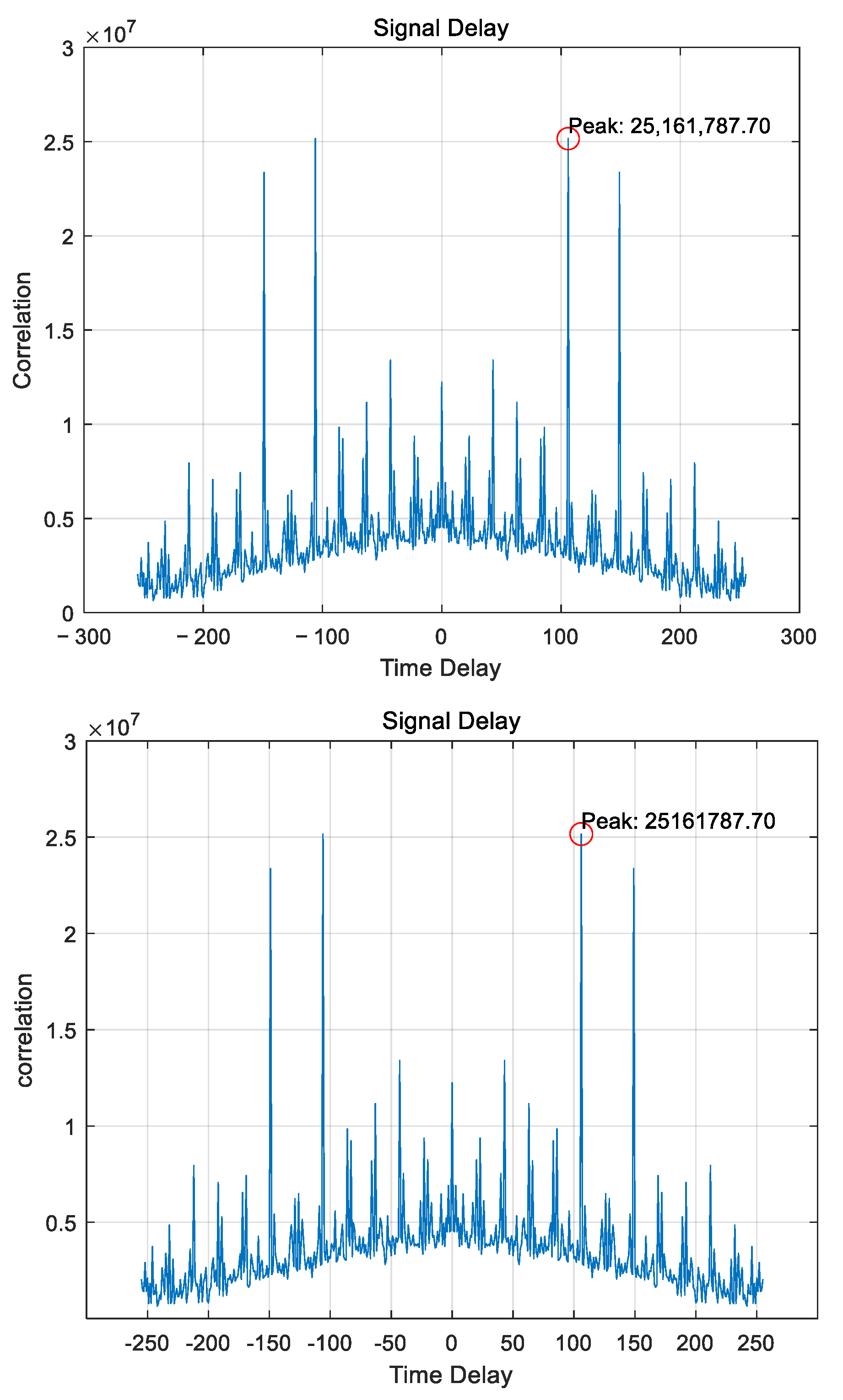
4.2.2. Optimization of the Cross-Correlation Method for Calculating the Rotation Factor

The actual echo signal from the piston is represented as $X\left(f\right)$, and the radar’s ranging echo signal within the cylinder is represented as $D\left(f\right)$. The cross-correlation function $R\left(f\right)$ in the frequency domain can be expressed as:

$$R\left(f\right)=X\left(f\right)\times D\left(f\right)$$

(10)

Selecting the dominant fundamental frequency in the cross-correlation function $R\left(f\right)$ involves the following steps:

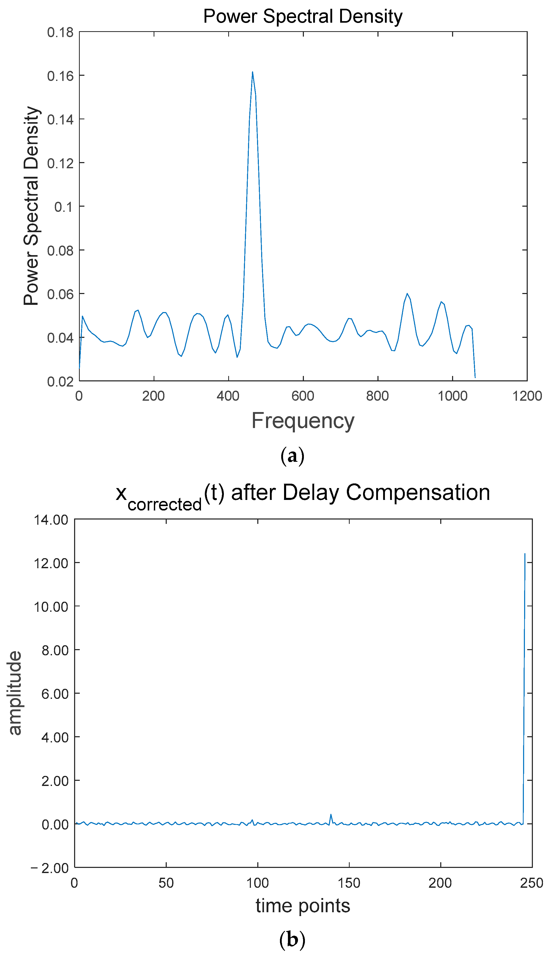
• The collected displacement signal is nonlinear and non-stationary, so the Welch method [20] is used to calculate the power spectral density:

  $$P\left(f\right)=\frac{R{\left(f\right)}^2}{L\times f_s}$$

  (11)

  where $P\left(f\right)$ represents the power spectral density at frequency $f$, representing the power distribution of the signal across various frequency components. $R\left(f\right)$ is the cross-correlation function in the frequency domain, $L$ is the length of $R\left(f\right)$, and $f_s$ is the sampling frequency (chosen to be twice the highest frequency component).

Assuming that the fundamental frequency component corresponds to the highest power spectral density value, the frequency component with a higher signal-to-noise ratio is caused by the fundamental frequency of the signal. Filtering out components with low signal-to-noise ratios entails eliminating those that are noise or non-fundamental frequency components, thereby more accurately identifying the fundamental frequency. Therefore, utilizing a signal-to-noise ratio threshold to filter power spectral density is instrumental in ascertaining the fundamental frequency.

2.

To calculate the signal-to-noise ratio based on signal power and noise power:

$$SN{R}_p=10\times \lg \left(\frac{P_{signal}}{P_{noise}}\right)$$

(12)

$P_{signal}$ represents the power of the signal, $P_{noise}$ represents the power of the noise, $SN{R}_p$ is the signal-to-noise ratio, and the power of the noise is calculated by computing the power in the frequency range where the signal does not contain useful signal.

In the threshold filtering method, to determine the fundamental frequency it is necessary to calculate the threshold based on the signal-to-noise ratio.

$$threshold=CO{F}^{-1}p$$

(13)

where $threshold$ is the threshold, $CO{F}^{-1}p$ is the inverse function of the cumulative distribution function of the signal-to-noise ratio data, percentile is denoted as p, representing the upper percentile in the signal-to-noise ratio distribution.

The threshold is modified based on the mean and standard deviation of the noise:

$$threshold=CO{F}^{-1}+\mu$$

(14)

where $\mu$ is the mean of the noise.

$$PS{D}_{filtered}\left(f\right)=\left\{\begin{array}{l}P\left(f\right)\hspace{1em}P\left(f\right)\rangle threshold\\ 0\hspace{1em}\hspace{1em} P\left(f\right)\langle threshold\end{array}\right\}$$

(15)

where $PS{D}_{filtered}\left(f\right)$ is the power spectral density after threshold filtering. If $P\left(f\right)$ exceeds the threshold, the point is retained; if $P\left(f\right)$ is less than or equal to the threshold, it is set to 0. Since the signal typically has higher power at its fundamental frequency and main harmonics, applying a threshold can help emphasize these components while reducing the noise level at other frequencies.

Find the maximum value: in $PS{D}_{filtered}\left(f\right)$, identify the point with the maximum amplitude, and the corresponding frequency is the fundamental frequency $f_{base}$.

For the fundamental frequency, using the least squares fitting to calculate the rotation factor involves the following steps:

• tract the time points and amplitude values corresponding to the fundamental frequency $f_{base}$.
• Define the fitting model:

  $$Q=A\ast \sin \left(w\ast t+z\right)$$

  (16)

  where $A$ is the amplitude,$w$ is the frequency, $t$ is time, and $z$ is the phase.
• Construct an error function to measure the difference between the fitting model and the actual data. The error function is defined as the mean square error (MSE) between the fitting model and the collected cross-correlation function data.

  $$E={\displaystyle \sum {\left(f_{base}-Q\right)}^2}$$

  (17)

  where $Q$ is the computed result of the fitting model.
• Use the least squares method for fitting by adjusting the parameters $A$, $z$, and $w$ in the fitting model to minimize the error function.
• Calculate the rotation factor:

From step 4, calculate $A_{estimated}$, $z_{estimated}$ and $w_{estimated}$ that minimize the error function. Obtain the complex form of the rotation factor:

$$M=A_{estimated}\times \exp \left(i\times z_{estimated}\right)\times \exp \left(i\times w_{estimated}\times t\right)$$

(18)

where $i$ is the imaginary unit, and $t$ is time.

4.3. Generating Delay Correction Signal Based on Rotation Factor

Multiplying by the rotation factor involves multiplying the cross-correlation sequence in the frequency domain by a certain rotation factor, according to the formula:

$$Q\left(f\right)=R\left(f\right)\times M$$

(19)

where $M$ represents the rotation factor.

Performing an Inverse Fast Fourier Transform (IFFT) on the cross-correlation function results in the time-domain cross-correlation function $r\left(t\right)$:

$$r\left(t\right)=F^{-1}\left\{Q\left(t\right)\right\}$$

(20)

where $F^{-1}$ represents the Inverse Fourier Transform. The signal obtained after IFFT represents relative displacement (i.e., time shift) rather than the absolute position of the signal. In other words, this result inherits the influence of the rotation factor.

Finally, in the obtained rotated cross-correlation function $r\left(t\right)$, peak detection is performed on the cross-correlation function to obtain the delay value $k$, which corresponds to the time delay at the peak position of the cross-correlation function.

Utilizing time correction and Fourier transformation to obtain the delay-compensated signal data $D_{corrected\left(t\right)}$:

$$D_{corrected\left(t\right)}=D\left(t-k\right)$$

(21)

where $D\left(t-k\right)$ represents the result of shifting the signal $x\left(t\right)$ backward along the time axis by $k$. By performing time shift correction for each time point, the peaks of the signal or specific events can be aligned with the actual occurrence time.

4.4. SVR Model Parameter Optimization

For nonlinear signals, direct linear models are unable to provide satisfactory compensation effects. SVRintroduces kernel functions to transform the data into a high-dimensional feature space, where the originally nonlinear relationships may become linearly separable.

For SVR (Support Vector Regression), it is necessary to use the $\epsilon$-epsilon-insensitive loss function, which is defined by the following equation:

$$L_{\epsilon }\left(y\right)=\left\{\begin{array}{l}0\hspace{1em}\hspace{1em}\hspace{1em}\hspace{1em} \left|f\left(x\right)-y\right|<\epsilon \\ \left|f\left(x\right)-y\right|<\epsilon \left|f\left(x\right)-y\right|\ge \epsilon \end{array}\right\}$$

(22)

In this context, $\epsilon$ is referred to as the insensitivity coefficient, which controls the fitting accuracy of the model. When the calculated error is less than $\epsilon$, the error can be considered negligible. However, when the error is significant, the impact of the error must be taken into account. Therefore, setting an appropriate insensitivity loss coefficient $\epsilon$ can ensure both the fitting accuracy and the generalization performance of the fitting problem. The linear regression plane is also expressed as: $f\left(x\right)=w^{T}x+b$. In this context, the explanations and classifications of $w$ and $b$ are the same. When using $f\left(x\right)$ to fit the sample data, it is assumed that the fitting error precision of all training data is $\epsilon$, with the constraint being:

$$\left\{\begin{array}{l}{y}_i-w^T{x}_i-b\le \epsilon \\ w^T{x}_i+b-y\le \epsilon \end{array}\right.$$

(23)

where $i=1,2,\dots ,n$. Based on the principle of structural risk minimization, $f\left(x\right)$ must minimize $\frac{1}{2}{‖w‖}^2$. At this moment, considering the error in fitting, the relaxation factor ${\xi }_i,{\xi }_i^{*}\ge 0$ is introduced, and the constraint conditions are now as follows:

$$\left\{\begin{array}{l}{y}_i-w^T{x}_i-b\le \epsilon +{\xi }_i\\ w^T{x}_i+b-y\le \epsilon +{\xi }_i^{*}\end{array}\right.$$

(24)

where $i=1,2,\dots ,n$. To ensure that the empirical risk is minimized, the optimization objective function and constraints after introducing the relaxation factor of loss coefficients are as follows:

$$\min \frac{1}{2}{‖w‖}^2+C{\displaystyle \sum _{i=1}^n\left({\xi }_i+{\xi }_i^{*}\right)}$$

(25)

$$s.t.\left\{\begin{array}{l}{y}_i-w^T{x}_i-b\le \epsilon +\xi \\ w^T{x}_i+b-y\le \epsilon +{\xi }_i^{*}\\ {\xi }_i,{\xi }_i^{*}\ge 0\end{array}\right.$$

(26)

where $i=1,2,\dots ,n$. The penalty parameter $C$ is crucial for the predictive performance of SVR in fitting problems; hence, how to reasonably select the parameter $C$ is of utmost importance.

Introduce the Lagrange multiplier $\alpha$ to obtain the dual problem of Equations (25) and (26). The form of the dual problem is as follows:

$$\min \frac{1}{2}{\displaystyle \sum _{i,j=1}^n\left({\alpha }_i^{*}-{\alpha }_i\right)}\left({\alpha }_j^{*}-{\alpha }_j\right)x_i^T{x}_j-{\displaystyle \sum _{i=1}^n{\alpha }_i^{*}\left(y_i+\epsilon \right)-{\alpha }_j\left(y_i+\epsilon \right)}$$

(27)

$$s.t.{\displaystyle \sum _{i=1}^n\left({\alpha }_i^{*}-{\alpha }_i\right)=0}$$

(28)

where ${\alpha }_i,{\alpha }_i^{*}\in \left[0,C\right],i=1,2,\dots ,n$.

For nonlinear regression problems, the method of kernel functions is also adopted, mapping the nonlinear input samples to another high-dimensional space. In this high-dimensional space, linear SVR is used to fit the samples.

By applying the kernel function, the above problem becomes:

$$\min \frac{1}{2}{\displaystyle \sum _{i,j=1}^n\left({\alpha }_i^{*}-{\alpha }_i\right)}\left({\alpha }_j^{*}-{\alpha }_j\right)K{x}_i^T{x}_j-{\displaystyle \sum _{i=1}^n{\alpha }_i^{*}\left(y_i+\epsilon \right)-{\alpha }_j\left(y_i+\epsilon \right)}$$

(29)

$$s.t.{\displaystyle \sum _{i=1}^n\left({\alpha }_i^{*}-{\alpha }_i\right)=0}$$

(30)

where ${\alpha }_i,{\alpha }_i^{*}\in \left[0,C\right],i=1,2,\dots ,n$.

By defining the parameter space and constructing a hash table, the performance indicators calculated for parameter sets are stored in the hash table. The best-performing parameter combination is selected as the final choice. Combining the hash table with grid search can avoid redundant computations and enhance accuracy. The specific process is as follows.

Read the radar echo signal data $x(t)$, use EMD to decompose and reconstruct the signal of $x(t)$, construct a delay compensation module to process $x(t)$, yielding the delay-compensated $x_{corrected\left(t\right)}$ signal data, and employ Time Series Split cross-validation to partition the dataset of $x_{corrected\left(t\right)}$ based on time.

For radar echo signal data, there are strong time series characteristics. Time Series Split can comply with this kind of time dependence, ensuring that the information in the training data appears in chronological order. Given that the starting index of a given time series dataset is 0 and the ending index is $t-1$, calculate the index range for each cross-validation fold, where the starting index of the training set is 0, and the ending index of the training set is $k\times (t-1)/K$, where $K$ is the number of folds in cross-validation. The starting index of the validation set is $k\times (t-1)/K+1$. The ending index of the validation set is $(k+1)\times (t-1)/K$. The time series dataset can be divided into $K$ continuous folds, each fold containing a training set and a validation set.

Construct two hash tables. The first hash table is used to store the combinations of SVR parameters, with the key being a unique identifier (hash value) for the parameter combination, and the value being the corresponding set of parameters. The second hash table is used to store the performance metrics, namely the mean squared error between the compensation signal and the real signal, with the key being the unique identifier for the parameter combination, and the value being a pointer to the corresponding set of parameters in the first hash table.

Insert key-value pairs into the corresponding buckets of the hash table based on the hash function. Before inserting, check if the hash table has reached the load factor threshold.

$$\lambda =\frac{A}{B}$$

(31)

Here, $\lambda$ is the load factor, $A$ is the number of key-value pairs, and $B$ is the size of the hash table.

Load factor inspection: If the load factor exceeds the preset threshold, it indicates that the hash table has been overly populated and necessitates a size adjustment.

Hash table expansion: Increase the size of the hash table by doubling the number of buckets. This reduces the average fill factor of the buckets, minimizes hash collisions, and maintains stable performance.

Rehashing: After the expansion of the hash table, rehash the existing key-value pairs to ensure they are distributed in the new buckets.

Combining two hash tables uses a cross-linked list, where each node in the cross-linked list contains a key, a value, and a pointer to other key-value pairs with the same hash value. For the first hash table, insert the key-value pairs into the cross-linked list, with the key acting as a unique identifier for the parameter combinations and the value corresponding to the parameter combinations. For the second hash table, insert the key-value pairs into the cross-linked list, with the key acting as a unique identifier for the parameter combinations and the value being a pointer to the corresponding parameter combinations in the first hash table. Continue inserting key-value pairs; after completing the hash table expansion, keep inserting new key-value pairs to maintain the adaptability and stable performance of the hash table. Initialize the parameter combinations, including optimal penalty parameters and the EPSILON value. Incorporate them into the improved SVR model, compute performance metrics, and write them into a dynamic hash table. Implement hash table expansion and key-value pair insertion. Use a random grid search to find parameter combinations not existing in the hash table and incorporate them into the SVR model to compute performance metrics. Repeat the above steps until no new parameter combinations that do not exist in the hash table can be found.

5. Construction and Analysis of Measurement Platform

5.1. Radar Selection

The design of the ranging radar is based on a 120 GHz radar sensor, and the circuit consists of five main parts: the control and processing unit, the modulation signal generation unit, the radar transceiver integrated unit, the baseband processing unit, and the power unit. Following the signal process, the overall system framework is shown in Figure 5:

After the STM32 initializes, it configures the ADF4169 chip to generate a sawtooth wave modulation signal, which drives the VCO inside the 120 GHz radar sensor (a single-chip microwave integrated circuit) in a phase-locked loop (PLL) manner to complete the design of the radar front end. The millimeter-wave radar sensor completes the transmission of the frequency-modulated signal and the reception of the echo signal on the one hand, and on the other hand it outputs two orthogonal signals IF_I and IF_Q, both carrying distance information, in differential mode. Due to the weak output signal and external interference and modulation signal leakage, it needs to undergo intermediate frequency filtering and amplification, which is completed by the baseband processing unit. After filtering and amplification, the baseband signal, satisfying the optimal acquisition range of the STM32 internal ADC, is sampled at a certain sampling frequency, and the amplitude-frequency characteristics are analyzed by the STM32 to calculate the corresponding distance. Finally, it is output to the host computer in serial form.

5.2. Piston Accumulator Piston Displacement Signal Detection and Test Verification Device

To verify the effectiveness of the algorithm, an experimental platform is designed based on the ranging radar and piston accumulator, which is composed of a slide table, stepper motor, grating ruler, and other equipment. Specifically, regarding the components, the grating ruler is fixed to the slide table and placed in the cylinder of the piston accumulator, allowing for arbitrary movement back and forth. The middle part of the grating ruler is connected to the slide table via a connecting piece and a cross-guide rail slide table. Simultaneously, the data lines of the grating ruler and slide table are connected to the industrial computer. The metal piston is embedded in the groove and fixed through fixed screw holes. The ranging millimeter-wave radar is located at the front end of the slide table, and the stepper motor is connected to the end of the slide table via a connecting line. The stepper motor contains a connector for the connecting line, which is connected to the industrial computer. The industrial computer is responsible for controlling the cross-guide rail slide table, stepper motor, core board of the millimeter-wave radar, and grating ruler, enabling all components to work together.

Measurement process: Firstly, start the ranging millimeter-wave radar for initial displacement calibration to reduce detection errors. Then, use the industrial computer to start the slide table, grating ruler, and stepper motor. After the startup is complete, control the speed of the stepper motor through the industrial computer’s upper computer system to control the slide table’s speed and the displacement of the metal piston. Move the device so that it is in the most suitable detection position inside the cylinder, then adjust the parameters of the upper computer system of the industrial computer for different group tests. By moving the slide table, detect the piston displacement signal under different displacements, and calculate the piston displacement data through the upper computer. Meanwhile, the grating ruler, relying on the fixing piece between the grating ruler and the slide table, moves with the slide table. Its measurement value is the true data of the piston movement, which serves as experimental verification data. The experimental setup is shown in Figure 6.

5.3. Measurement Signal Analysis

For the selected detection signal, construct the frequency domain waveform using the FFT method, and for the noise use EMD for denoising. Using radar to collect displacement signals of the same type of analog piston as the reference signal, construct a time delay map, as shown in Figure 7.

The peak position is at 106.00, the peak intensity is 2.516 × 10⁷, and the peak width is 2.00. There is an actual delay of 106 units compared to the reference signal. To address this time delay, a delay compensation module is applied.

5.4. The Delay Compensation Module Analysis and Processing Are Performed

5.4.1. Analysis of Matched Filter Gain Processing

Using the matched filter gain algorithm mentioned above for processing, followed by a spectral analysis, it is found that there are a fewer number of peak values in the echo signal. Therefore, it is necessary to introduce a gain factor G into the output signal of the matched filter. The gain factor G is calculated by the algorithm mentioned above, as shown in Figure 8.

In the case of measuring object displacement, an appropriate gain factor G is determined by comparing the expected power with the actual power. The expected power is based on experimental measurements using a calibrated object with known position and displacement. The actual power is obtained by segmenting the signal in the frequency domain, calculating the power for each segment, and finally taking the average. The image with the gain factor added is shown in Figure 9.

According to the spectral analysis diagram, the increase in the number of echo signal peaks indicates that sufficient echo signals can be obtained.

5.4.2. For the Calculation of the Rotation Factor and the Generation of the Correction Signal in Section

The significant reflection on the metal surface of the cylinder can lead to an increase in the time delay of the echo signal, causing interference and confusion with the actual target signal. This interference can result in considerable deviations in parameters, such as distance, velocity, and direction. To address these issues, the cross-correlation method is employed to calculate the rotation factor and achieve time delay compensation.

Using the Welch method to calculate the power spectral density, the spectral analysis of the signal is optimized through segmentation, window function processing, and averaging periodograms. The fundamental frequency is determined by using the signal-to-noise ratio to filter the power spectral density with a threshold. The least squares fitting is used for the fundamental frequency to calculate the rotation factor and, finally, a time-delay corrected signal is generated based on the rotation factor, as illustrated in Figure 10.

5.4.3. The Comparison of Parameter Optimization

By calculation, the optimal parameters are obtained as $A_{estimated}=0.98392$, $z_{estimated}=3.649\times {10}^{-5}$, and $w_{estimated}=1.0456$. The optimal parameter set for the improved SVR is a penalty parameter of 10 and an Epsilon value of 0.01. To verify the effectiveness of the delay compensation measurement method, the compensation effect of the support vector machine is compared with the compensation effect after adding delay compensation. The processing results are shown in Figure 11.

Using denoised signal data, calculating the mean square error after compensating with support vector regression and rotation factor-based support vector regression methods is shown in

Table 2. Mean squared error after compensation.

Methods	MSE
SVR	7045.88
Rotation Factor and Support Vector Regression	0.09216

.

The test results indicate that, after using delay compensation, the mean square error of the energy accumulator piston displacement signal compensation method based on rotation factor support vector regression is lower than that without using delay compensation.

6. Conclusions

This article introduces a compensation algorithm for the displacement signal of a piston accumulator based on radar measurement. A device for detecting and verifying the displacement signal of the piston accumulator is designed. Metal pistons with different displacement amounts at a fixed scene are measured to investigate the influence of metal reflections inside the piston accumulator cylinder on radar measurement displacement signals. A delay compensation model for the influence of internal metal reflections is proposed.

By adding a device for detecting and verifying the displacement signal of the piston accumulator inside a piston accumulator with a diameter of 180 mm, multiple experiments were conducted, and preliminary conclusions were drawn. Factors such as metal reflections in the piston accumulator cylinder, measurement distance, and horizontal angle limitations cause time delays in radar measurement signals. Simply using support vector regression for radar displacement signal compensation is not obvious. However, with the addition of a delay compensation module, the compensation effect of the support vector regression model with a rotational factor for radar displacement signals is significantly improved.

References

1. Pichler, K.; Haas, R.; Kastl, C.; Plöckinger, A.; Foschum, P. Comparison of fault detection methods for a hydraulic accumulator loading circuit. In Proceedings of the 2020 IEEE Conference on Industrial Cyberphysical Systems (ICPS), Tampere, Finland, 10–12 June 2020; pp. 117–122. [Google Scholar]
2. Newton, G.F.; Aondona, T.I.; Chile, C.A. Design and implementation of a wireless fluid level display system using ultrasonic sensing technique. J. Eng. Res. Rep. 2020, 14, 30–40. [Google Scholar] [CrossRef]
3. Hong, X.; Zhang, B.; Liu, Y.; Qi, H.; Li, W. Deep-learning-based guided wave detection for liquid-level state in porcelain bushing type terminal. Struct. Control Health Monit. 2021, 28, e2651. [Google Scholar] [CrossRef]
4. Hu, M.; Wang, F.; Chen, L.; Huo, P.; Li, Y.; Gu, X.; Chong, K.L.; Deng, D. Near-infrared-laser-navigated dancing bubble within water via a thermally conductive interface. Nat. Commun. 2022, 13, 5749. [Google Scholar] [CrossRef] [PubMed]
5. Schenkel, F.; Baer, C.; Rolfes, I.; Schulz, C. Plasma state supervision utilizing millimeter wave radar systems. Int. J. Microw. Wirel. Technol. 2023, 15, 1001–1011. [Google Scholar] [CrossRef]
6. Liu, P.; Chen, Z.; Gui, W.; Yang, C. High-Precision Real-Time Detection of Blast Furnace Stockline Based on High-Dimensional Spatial Characteristics. Sensors 2022, 22, 6245. [Google Scholar] [CrossRef] [PubMed]
7. Yuan, H.; Zhang, Z.; He, X.; Wen, Y.; Zeng, J. An Extended robust estimation method considering the multipath effects in GNSS real-time kinematic positioning. IEEE Trans. Instrum. Meas. 2022, 71, 1–9. [Google Scholar] [CrossRef]
8. Wang, Z.; Chen, X.; Ning, X. BER analysis of integrated WFRFT-OTFS waveform framework over static multipath channels. IEEE Commun. Lett. 2020, 25, 754–758. [Google Scholar] [CrossRef]
9. Khodarahmi, M.; Maihami, V. A review on Kalman filter models. Arch. Comput. Methods Eng. 2023, 30, 727–747. [Google Scholar] [CrossRef]
10. He, T.; Tian, B.; Wang, Y.; Li, S.; Xu, S.; Chen, Z. Joint ISAR imaging and azimuth scaling under low SNR using parameterized compensation and calibration method with entropy minimum criterion. EURASIP J. Adv. Signal Process. 2023, 2023, 1–20. [Google Scholar] [CrossRef]
11. Ju, M.; Dai, Y.; Han, T.; Wang, Y.; Liu, X. Improved Compressed Sensing Reconfiguration Algorithm with Shockwave Dynamic Compensation Features. Shock. Vib. 2022, 2022, 4035279. [Google Scholar] [CrossRef]
12. Yang, Z.; Liu, D.; Zheng, G. Roll Eccentricity Signal Detection and Its Engineering Application Based on SFFT-IAA. Appl. Sci. 2022, 12, 8913. [Google Scholar] [CrossRef]
13. Gao, S.; Xu, L.; Li, Y.; Ji, J. Roll eccentricity extraction and compensation based on MPSO-WTD and ITD. PLoS ONE 2022, 17, e0259810. [Google Scholar] [CrossRef] [PubMed]
14. Li, J.; Jiang, L.; Yu, F.; Zhang, Y. Research on improving measurement accuracy of acoustic transfer function of underwater vehicle. MATEC Web Conf. 2021, 336, 01006. [Google Scholar] [CrossRef]
15. Li, Y.; Wu, J.; Mao, Q.; Xiao, H. A Novel Two-Dimensional Autofocusing Algorithm for Real Airborne Stripmap Terahertz Synthetic Aperture Radar Imaging. IEEE Geosci. Remote Sens. Lett. 2023, 20, 4012405. [Google Scholar] [CrossRef]
16. Cheng, T.-Y.; Wang, W.-Y.; Li, J.-S.; Guo, J.-X.; Liu, S.; Lü, J.-Q. Rotational Doppler effect in vortex light and its applications for detection of the rotational motion. Photonics 2022, 9, 441. [Google Scholar] [CrossRef]
17. Teja, K.; Tiwari, R.; Mohanty, S. Adaptive denoising of ECG using EMD, EEMD and CEEMDAN signal processing techniques. J. Phys. Conf. Ser. 2020, 1706, 012077. [Google Scholar] [CrossRef]
18. Gorji, R.T.; Hosseini, S.M.; Abdoos, A.A.; Ebadi, A. A hybrid intelligent method for compensation of current transformers saturation based on PSO-SVR. Period. Polytech. Electr. Eng. Comput. Sci. 2021, 65, 53–61. [Google Scholar] [CrossRef]
19. Ma, Z.; Choi, J.; Yang, L.; Sohn, H. Structural displacement estimation using accelerometer and FMCW millimeter wave radar. Mech. Syst. Signal Process. 2023, 182, 109582. [Google Scholar] [CrossRef]
20. Jwo, D.J.; Chang, W.Y.; Wu, I.H. Windowing techniques, the welch method for improvement of power spectrum estimation. Comput. Mater. Contin. 2021, 67, 3983–4003. [Google Scholar] [CrossRef]
Figure 1. Assembly diagram of piston-type accumulator.
Processes 12 01036 g001
Figure 2. FMCW Radar System Block Diagram.
Processes 12 01036 g002
Figure 3. Frequency Modulation Curve of an FMCW Signal.
Processes 12 01036 g003
Figure 4. FMCW Signal Target Distance Calculation Diagram.
Processes 12 01036 g004
Figure 5. Overall Design Diagram.
Processes 12 01036 g005
Figure 6. Measurement platform (a) Measurement of the environment; (b) Displacement measurement device.
Processes 12 01036 g006
Figure 7. Comparative Time-Delay Maps.
Processes 12 01036 g007
Figure 8. (a) The gain of the matched filter. (b) Spectral Analysis.
Processes 12 01036 g008
Figure 9. (a) Image after increasing the gain factor. (b) Spectrum analysis.
Processes 12 01036 g009
Figure 10. (a) Power spectral density. (b) The signal after delay compensation.
Processes 12 01036 g010
Figure 11. (a) Comparison between compensated signal using support vector regression and real signal for the original signal; (b) Comparison between compensated signal using rotation factor-based support vector regression and real signal for the original signal.
Processes 12 01036 g011