Abstract
In this paper, an online energy-saving control allocation strategy based on self-updating loss estimation for multi-motor drive systems is proposed, where the impact of variations in motor parameters and distribution coefficients is considered. Firstly, a drive system model for multi-motor drive systems incorporating iron loss in permanent magnet synchronous motor (PMSM) is established. Then, a self-updating PMSM loss estimation method based on dynamic torque–current mapping is proposed. The torque–current mapping is initially identified based on the conv-fusion curve, and iteratively updated by optimal estimation. Subsequently, an online control allocation method based on line search is proposed, which mitigates the adverse effects caused by variations in distribution coefficients and reduces the total motor loss. Finally, the effectiveness of the proposed strategy is verified on the hardware-in-the-loop (HIL)-based platform. The results demonstrate that the strategy effectively enhances energy efficiency while maintaining the original control performance of the system.
1. Introduction
With the development of various electric drive systems such as cars, trains, and airplanes, energy consumption is also rising annually [1,2]. Hence, it is imperative to reduce energy consumption and advocate for sustainable development. In a multi-motor drive system, the control input solution of the motion equations is not definite, and this problem needs to be solved through control allocation. Given that motor efficiencies vary with torque and speed, total losses can be minimized by optimizing motor allocation [3].
Research on energy-saving-oriented control allocation is primarily categorized into rule-based [4,5] and optimization-based [6,7] strategies. In existing rule-based researches, Yuan [8] established the second-order loss function using the motor loss separation model and showed that uniformly dispersing the total torque to each motor may minimize the overall power loss. Similarly, Yu [9] and Gu [10] also concluded that evenly distributed torque is optimal. Song [11] considered the inconsistency of the motor in torque distribution and proposed an equivalent loss control allocation strategy. Nevertheless, considering the performance variations across motors and the complexity of losses in various operating situations, relying only on the second-order loss function may not accurately depict the actual loss. Thus, while the rule-based control allocation approach is simple to implement, its energy-saving potential is limited, necessitating the adoption of optimization-based control allocation strategies.
Dizqah [12] developed a multi-dimensional torque distribution ratio lookup table using the total power loss curve and a multi-parameter quadratic programming method to address the optimal energy-saving torque allocation issue in vehicles. Torinsson [13] and He [14], respectively, utilized quadratic programming and model predictive control for torque allocation through offline optimization. However, these approaches could not adequately take into consideration variations in motor parameters during real-time operation.
Parra [15] implemented parallel optimization of electric vehicle yaw rate and wheel energy-saving torque allocation using nonlinear model predictive control and used dynamic programming to solve the optimization problem. Gao [16] and Liu [17] also utilized dynamic programming methods to solve the torque allocation issue in electric vehicles. The effect is substantial but necessitates extensive computation and lacks real-time performance. Wei [18,19] attempted to enhance the speed and efficiency of the optimization process by employing a customized gradient method and an enhanced particle swarm optimization (PSO) method. Wang [20] used the offline optimized torque allocation results as the starting point for the online particle swarm algorithm optimization in the energy-saving torque optimization process for electric vehicles to accelerate the solution process. Jiang [21] implemented energy-efficient control allocation for six-wheel autonomous vehicles using a seeker optimization algorithm (SOA). However, trains have more control variables compared to electric vehicles, which makes it difficult for some of the search-based and heuristic optimization algorithms to converge in a short amount of time.
Based on the above discussion, most optimization-based control allocation research is undertaken with the assumption that motor parameters remain constant. The economic optimization objectives of permanent magnet synchronous motors (PMSMs) [22] rely mainly on simulation or experimental data, such as efficiency maps [23], polynomial fitting, or unfitted loss curves [12], and it is difficult to calculate the loss based on the real-time identification parameters of the motor during operation. The above methods will lead to inaccurate distribution results and limit the energy-saving potential of the system. Furthermore, there are few mechanism-based loss estimating methods [8,9,10] available that can estimate loss using motor parameters. However, these methods are primarily designed for surface-mounted PMSMs, which are not suitable for more commonly used embedded PMSMs.
This paper proposes an online control allocation strategy for train multi-motor drive systems, designed to adapt to real-time variations in motor parameters. Our approach includes developing a method to estimate the losses of a PMSM that accounts for parameter variations and designing a stable online optimization algorithm capable of managing more control variables to mitigate the adverse effects of fluctuations in system distribution coefficients. To this end, focusing specifically on the train’s multi-motor drive system, an online energy-saving control allocation strategy based on self-updating loss estimation for a multi-motor drive system is proposed. To sum up, the main contributions of this article are as follows.
- A self-updating PMSM loss estimation method based on dynamic torque–current mapping is proposed. The torque–current mapping is initially identified based on the conv-fusion curve, and is iteratively updated based on optimal estimation. This method retains a direct correlation between motor loss and parameters and enjoys extensive flexibility in motor control methods, effectively addressing the challenge of promptly estimating PMSM loss through various motor parameters.
- A novel online control allocation method based on line search is proposed. This method leverages the descent method, incorporating the Armijo criterion and backtracking to determine an optimal step size, and an initial search value of it is designed to regulate torque changes. With these designs, the method can effectively reduce total motor loss and mitigate the impact of variations in distribution coefficients, and thus maintains real-time performance.
The remaining sections are organized as follows. Section 2 provides the details of the drive system model for trains. In Section 3, the self-updating loss estimation method is described. A thorough introduction of the control allocation method is presented in Section 4. In Section 5, the effectiveness of the proposed control allocation strategy is verified. This paper concludes in Section 6.
2. Drive System Composition and Modeling
The multi-motor drive system of trains employs a multi-layer control structure. The drive system consists of 16 power units, which are composed of three-phase inverters and PMSMs. Each power unit is controlled by its corresponding traction control unit. In trains, the upper-level controller used for calculating the total demand torque is referred to as the central control unit. It computes the train’s total demand torque through a pre-designed traction curve, which uses train speed as the independent variable. The central control unit calculates the total torque based on the train speed and traction curve. Then, the total demand torque is allocated to 16 traction control units through a control allocation unit. Finally, the motors utilize this reference torque as the control input to produce electromagnetic torque, which in turn provides traction for the train.
2.1. PMSM Modeling Considering Iron Loss
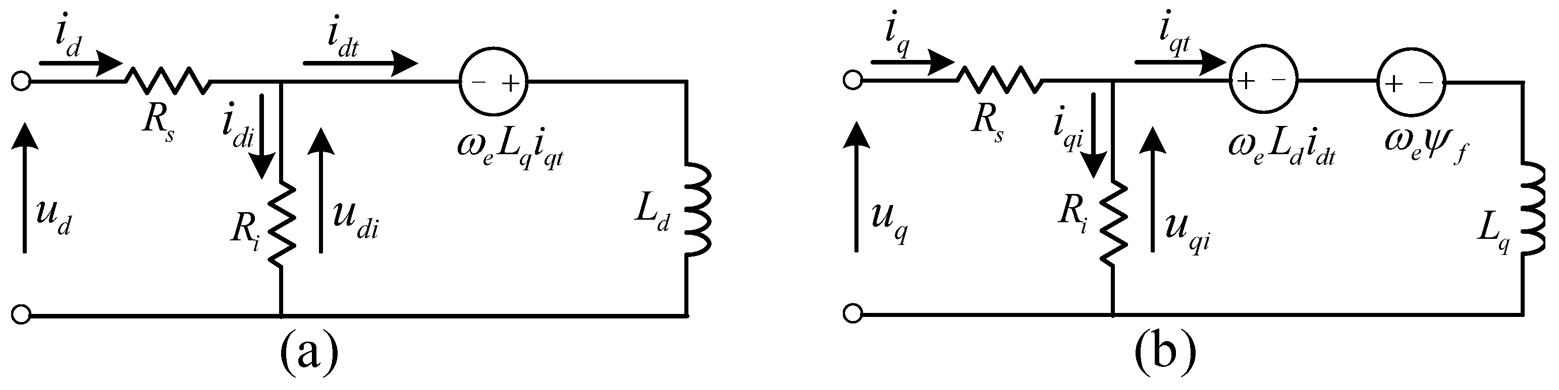
In an equivalent circuit model considering the iron loss of a PMSM, the iron core loss and rotor eddy current loss can be represented by the iron loss resistance . is the resistance of the stator, which is related to the copper loss. The equivalent circuit diagram of the PMSM considering iron losses is shown in Figure 1 in the dq coordinate system, where and mean voltage components of the dq-axis, and mean current components of the dq-axis, and mean torque components of the dq-axis current, and and mean iron loss components of the dq-axis currents.

Figure 1.
Equivalent circuit diagram of PMSM in the dq-axis coordinates: (a) Equivalent circuit diagram of PMSM under d-axis coordinates. (b) Equivalent circuit diagram of PMSM under q-axis coordinates.
According to Figure 1, the dynamic voltage equation and torque equation can be formulated below.
where represents electrical angular velocity of the rotor, represents flux linkage of permanent magnet, and are inductance of the d-axis and q-axis, respectively, is the number of pole pairs of the motor, and p represents the differential operator.
The PMSM copper losses and iron losses are expressed as follows.
and in the steady state. According to Equation (1), dq-axis torque components and iron losses current components in the steady state can be obtained and expressed as
Therefore, the losses and torque expressions of the PMSM can be rewritten as follows.
where , , , and .
2.2. Drive System Modeling
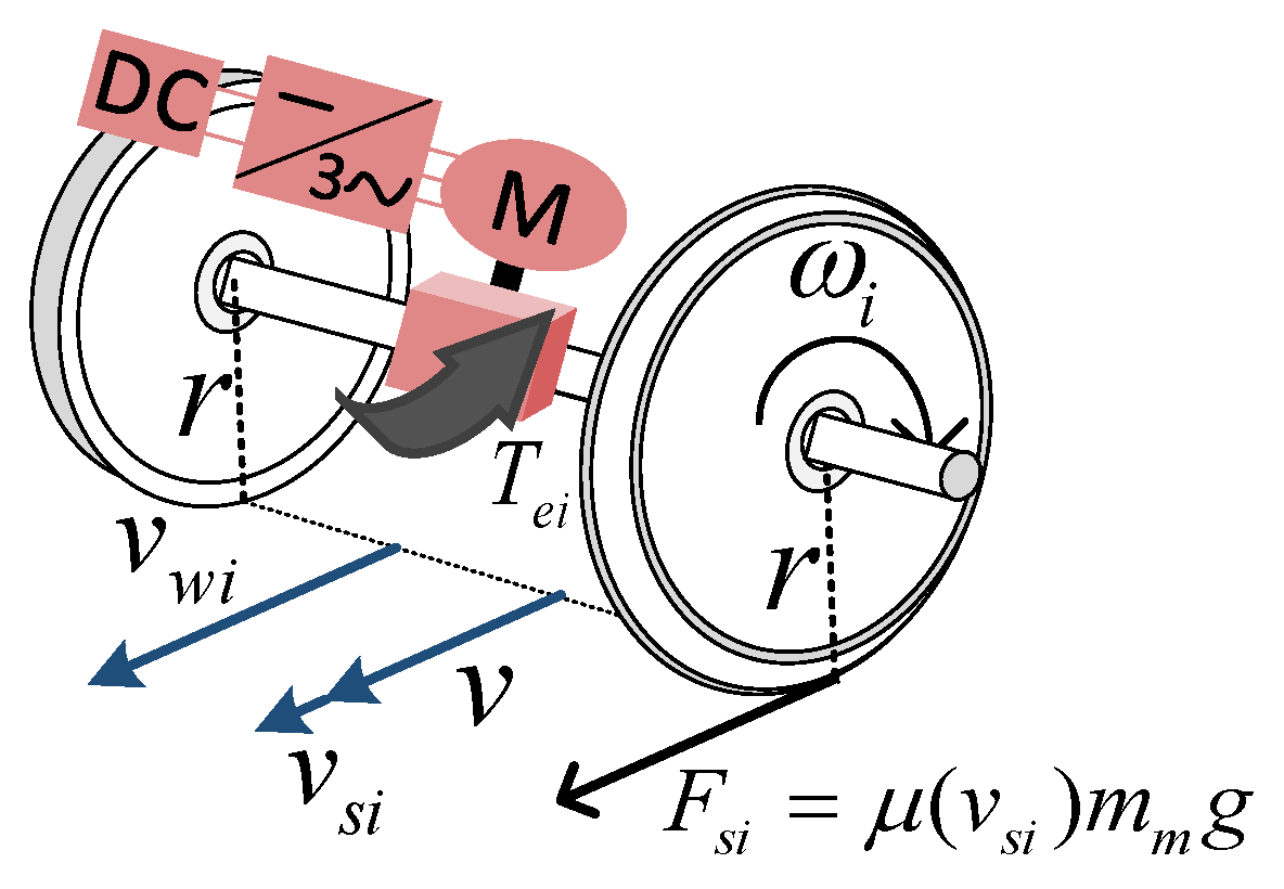
This paper only analyzes the longitudinal motion of the train because the lateral motion is not controlled by a power unit. The module depicted in Figure 2 consists of a power unit and a wheelset. For the i-th motor, the motor generates electromagnetic torque , which propels the wheelset and produces an angular velocity . Consequentially, the angular velocity of the wheelset results in a linear velocity at the outer edge of the wheelset, which differs from the train speed v. This difference is measured as the creep speed . The adhesion coefficient is a factor that depends on the creep speed. It is multiplied by the positive pressure of the train on the track to determine the traction force produced by this module. This traction force is also responsible for the actual load on the motor. The above process can be described as follows.
where the subscript i represents the i-th motor, and mean the electrical angular velocity and equivalent rotational inertia of the i-th motor, r means wheel radius, means positive pressure of module, and a mean transmission efficiency and ratio of gear, respectively, and , , and are constants.

Figure 2.
Schematic diagram of train wheelset dynamics model.
After determining Equation (8), the actual mechanical motion equation of the motor can be obtained as
The traction force generated by the i-th motor is recorded as . The traction force of each motor acts on the train together, which can be expressed as
where M represents train mass, represents the fundamental resistance of the train, which is determined by the train speed v and M. Therefore, the state space equation of the angular velocity of each wheelset and the train speed in the drive system can be expressed as follows.
where and represent differentiation of state variables of angular velocity of the i-th motor and train speed respectively.
3. Self-Updating Loss Estimation of PMSM
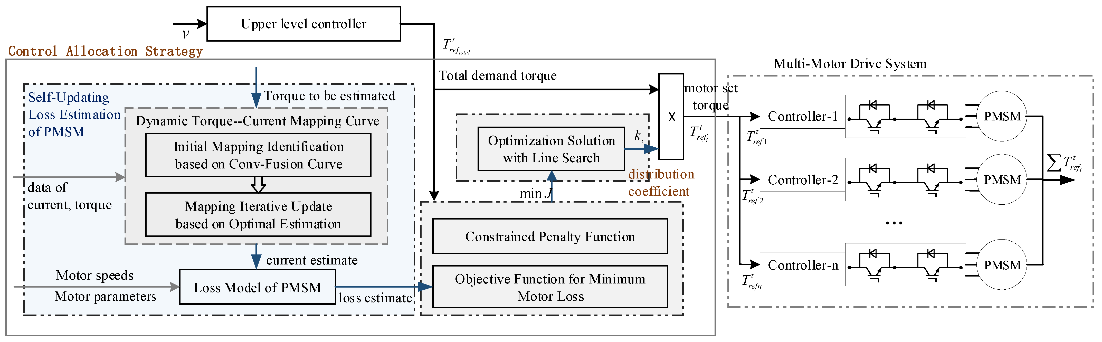
The implementation diagram of an online energy-saving control allocation strategy based on self-updating loss estimation for multi-motor drive systems is shown in Figure 3. In this section, the self-updating loss estimation part shown in the blue box of this figure will be elaborated in detail, and the establishment of optimization objectives and the optimization solution will be discussed in Section 4.
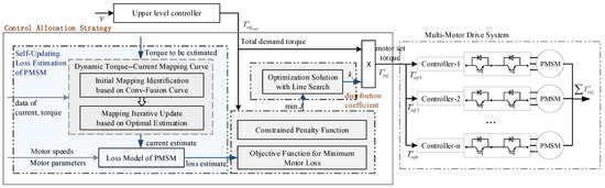
Figure 3.
Overall implementation diagram of control allocation strategy in the multi-motor drive system of the train.
Considering the variability of motor parameters during operation, there is a need to propose a parametric motor loss estimation method. In current research, estimating techniques relying on loss data are limited to specific parameter configurations, hindering the ability to directly connect loss with motor parameters. Furthermore, current mechanistic estimating methods do not adequately account for the complexities of the torque and current relationships across various motor control techniques. To overcome these limitations and provide accurate and flexible economic optimization goals for online control allocation strategies, this section attempts to create a decoupled, demand torque-variable-based parametric online estimating method for PMSM loss.
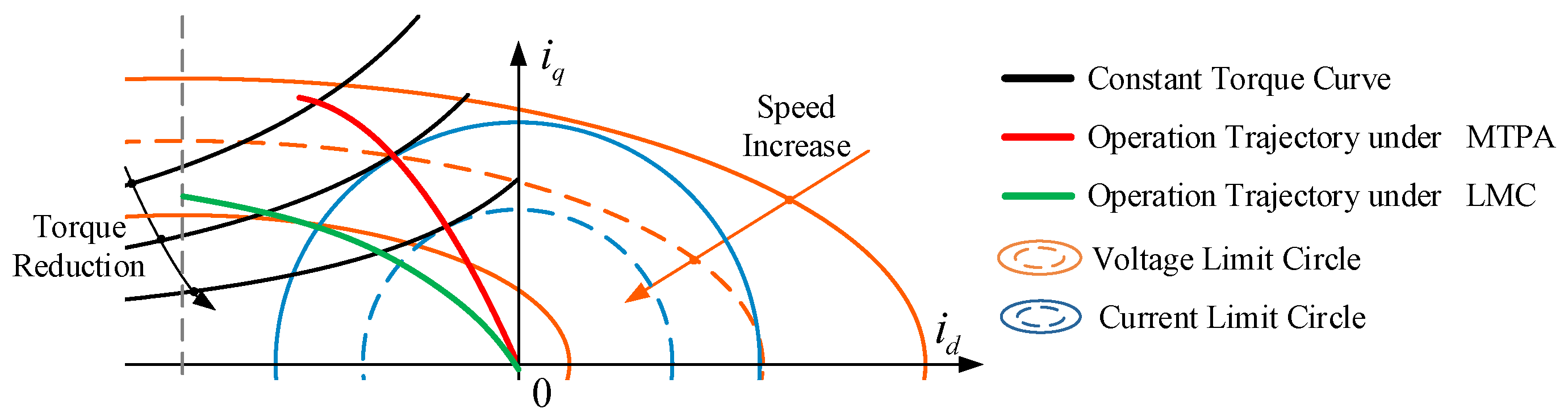
Figure 4 depicts the operating trajectories of embedded PMSMs in different motor control methods, demonstrating a one-to-many relationship between motor torque and dq-axis currents with the selected motor control method. The accuracy of motor loss estimation is greatly influenced by the motor control mechanism due to the direct association between motor loss and operating currents. Moreover, motors utilizing hybrid switching or parameter-adaptive control methods shift their operating trajectories according to operating circumstances and motor performance, leading to alterations in the correlation between motor loss and torque.
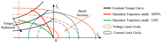
Figure 4.
Schematic diagram of the operation trajectory of embedded PMSMs under different control strategies.
Based on the above discussion, this section proposes a two-stage motor loss estimation method that relies on a mechanistic model and incorporates real-time system sampling data. This method decouples motor loss estimation into two independent steps: estimating the dq-axis currents from the total demand torque, and then converting these currents into motor losses. The relationship between current and motor loss, as detailed in the previously mentioned drive system mechanistic model, maintains the direct influence of motor parameters on loss. Regarding current estimation, due to the variety of motor control methods, it is difficult to immediately derive explicit expressions from the mechanistic model. Therefore, a data-based approach to identify the dynamic torque–current mapping curves is adopted in this paper. Given the motor’s low rotational inertia and high response speed, this paper has decided to disregard the impact of system inertia. Instead, real-time sampling data are used directly to construct dynamic torque–current mapping curves, accurately depicting the relationship between torque and current under current operating conditions [24].
3.1. Initial Mapping Identification Based on Conv-Fusion Curve
The identification of dynamic torque–current mapping unfolds in two stages: initial mapping identification and the continuous update of the mapping results obtained from the initial identification. Dynamic torque–current mapping can be decomposed into two independent curves, namely and . By utilizing multiple sets of torque–current data pairs collected from the system, which include noise, the process of mapping acquisition is transformed into the problem of fitting two curves within a two-dimensional coordinate system.
As an integral part of the online control allocation strategy, ensuring the real-time aspect of curve fitting is critical. Additionally, to reduce the impact of noise and enhance the accuracy of system energy loss estimation, improving curve smoothness is essential. Therefore, it is necessary to adopt a fitting method that is computationally convenient, offers high fitting accuracy, and ensures curve smoothness.
Given that the mapping curves lack typical functional form characteristics, it is difficult to fit them with specific functions. Neural network-based approaches [25] may fulfill accuracy and smoothness criteria but are not practical for real-time applications because of their high computing complexity. Furthermore, methods that rely on full torque range data not only have long sampling times but are also prone to overfitting. However, the mapping curves have distinct linear features within certain intervals. Therefore, piecewise linear fitting effectively circumvents the aforesaid problems, enhancing both precision and computing efficiency. As a result, this part proposes a curve convolution fusion method based on piecewise linear fitting to achieve a smooth transition between two straight line segments.
To provide a more precise depiction of the curve, a series of torque and currents data is obtained at uniform intervals spanning from 0 to the motor maximum output torque. The torque corresponding or value is denoted as . Figure 5 is a schematic diagram of curve convolution fusion, where curve L represents the originally fitted curve, and represents the newly fitted curve in the current period. The elucidation of the particular approach for implementation is provided as follows.
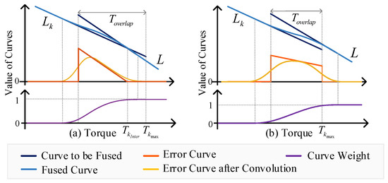
Figure 5.
Schematic diagram of curve convolution fusion: (a) Two lines have an intersection in the overlapping area. (b) Two lines do not have an intersection in the overlapping area.
The core technique of the proposed curve fusion method lies in allocating gradual transition weights to the two linear segments of the area to be fused. This method smooths and diffuses by conducting vector convolution operations on the difference between the two linear segments. Subsequently, the error curve after convolution is integrated and normalized to determine the curve weight at certain places. The specific implementation strategy is as follows.
During the process of train traction, the output torque of each motor gradually diminishes following the traction curve, generating sample data of torque, d-axis current and q-axis current that encompasses a significant portion of the torque range. The system sampling data are acquired at a fixed time interval , and the duration taken for each m number of samples is recorded as a time interval. In the k-th time interval, the sampled data set is obtained, where m is the number of data in the data set . The range of torque values represented in the sampling data is denoted as . A least squares linear fitting is applied to the data set , resulting in the determination of linear fitting parameters as
As a result, the fitted curve can be described as : , where represents the ordinate of the curve , meaning d-axis or q-axis current, T represents the abscissa of the curve , meaning torque. The torque range represented by is extended from the original curve L to the newly adjusted curve , which is the area where the two curves overlap. Assume that there is an intersection point between two curves, and the torque corresponding to the intersection point is recorded as , then calculate the curve difference in the torque range , as shown in Figure 5a. Otherwise, it can be considered that , and the torque area range for calculating the curve difference is , as depicted in Figure 5b.
The error is calculated by making a difference between the data points of the curves and L in the overlapping area. Then, Gaussian window function is applied to operate vector convolution on the error so that the error propagates to the surrounding area and becomes smooth. The above process is described as follows.
where represents the result of the originally fitted curve at time k, represents the result of error after Gaussian smoothing, u in Equation (14) is the input of the Gaussian window function, and is its standard deviation, which is used to control the width of the window.
The data closing to one curve at both ends of the fusion region should possess greater confidence and carry a higher weighting compared to the data associated with the curve at the other end. The difference curve, which has been smoothed using convolution, is subjected to integration and normalization. The resulting value is then employed as the weight for the curve, which is expressed as
where is the weight curve, and T means torque, which is the independent variable of the weight curve. Therefore, the description of the mapping curve L is changed as
where represents the result of the updated curve L, represents the ordinate of the torque–current mapping curve.
3.2. Mapping Iterative Update Based on Optimal Estimation
Considering the time-varying characteristics of the torque–current mapping curve affected by the motor control method, this paper locally updates the torque–current mapping curve using the latest sampling data to enhance the accuracy of loss estimation. The newly sampled data contains a large amount of noise, and its deviation may not only be from changes in the motor’s operating trajectory but also from other random factors, leading to insufficient data reliability. Hence, it is essential to devise an effective method to fuse the new sampling data with the existing mapping curve, ensuring a seamless alignment between the updated mapping curve and the new sample point.
Directly incorporating new sampling points for refitting does not facilitate maintaining computational simplicity, nor does it adequately consider the credibility of new data during the updating process. This paper introduces the concept of data fusion from the Kalman filter theory, implementing an optimal estimation based on the minimum standard deviation within the original mapping interval and new sampling data.
Kalman filter is a classical mathematical method [26] for state estimation, capable of obtaining optimal estimates of unknown quantities from noisy data. Although curve updating is not its traditional application field, the core concepts of optimal estimation and data fusion are still worth adopting in curve updating. Consider the state variables , which represents a series of dq-axis currents in the mapping curve L results, is the state variables at the k-th time, where n represents dimension of state vector, also the number of coordinate points used to describe the mapping curve. The state equation and observation equation of the system are formulated below.
where represents the identity matrix, represents the observation results in the k-th time interval, and represent the corresponding system noise and measurement noise, respectively, and their covariances are recorded as and , respectively.
Assumes that both system noise and measurement noise follow Gaussian distributions. Observation noise and system prediction equation noise can be considered to be related to the sampling point density and the error between the sampling points and the original points, respectively. Based on this, the covariance matrix of each noise can be constructed. The specific implementation is as follows.
Once the new sampling data set has been acquired, the density estimation of the data is performed using the Gaussian kernel function. This allows us to obtain the density estimate for each sampling point, as shown below. Next, the sampling point and its corresponding original mapping curve are subjected to linear interpolation. The resulting interpolated curve is then compared to the original curve to calculate the error .
where m is the number of sampled data set ; h is a constant parameter in the Gaussian kernel function.
The sampling point density and error mean are calculated within the range of , as the density and error at . The aforementioned procedure is depicted as follows.
where represents the total number of data in the range near , represents the corresponding average density, and represents the corresponding average error, , when · is true and when · is false. Then, convolution is employed to effectively smooth and propagate the density and error, in the same way as Equation (14), and and are obtained, respectively. As a result, the covariance matrix of the system noise and measurement noise at k-th time intervals can be expressed as follows.
The optimal estimate of the mapping curve in differential form can be expressed as
where is a priori estimate at k-th time interval, calculated by , is called gain at k-th time interval. Therefore, the error of the estimate is expressed as
where , is called a priori state error. The covariance matrix of the estimation error is expressed as
where , . The covariance matrix of a priori state error is calculated by
In the optimal estimate representation shown in Equation (24), the gain needs to be determined. To minimize the covariance matrix of the estimation error , the gain should be calculated as
Therefore, the optimal estimate of the state variable can be obtained according to Equations (24)–(28).
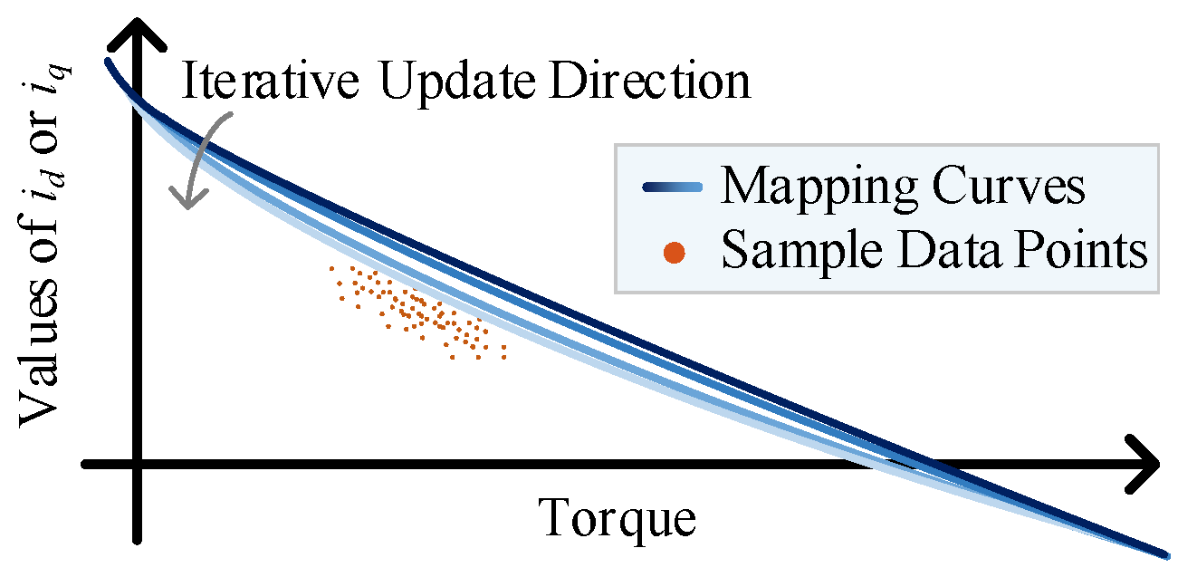
In the implementation process, the mapping update and the initial mapping identification use the same update interval to perform a local update operation. As depicted in Figure 6, assuming that the data points sampled within a certain time interval deviate from the mapping curve, the mapping curve needs to approach the new sampling point smoothly and gradually. If the sampling points of multiple consecutive time intervals are of this type of distribution, the mapping curve will pass through the area of the sampled data, as illustrated in Figure 6. Conversely, if the sampling points that deviate from the mapping curve are due to sporadic factors within a certain time interval, the mapping curve will not exhibit significant deviations.
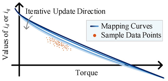
Figure 6.
Schematic diagram of curve iterative update based on optimal estimation.
3.3. Loss Estimation of PMSM
After the initial identification and iterative updating of the torque–current mapping, a dynamic mapping relationship that can automatically adjust based on the operating condition is obtained, denoted as . The current to motor loss calculation formula described by Equations (5) and (6) is denoted as , thus, the two-stage loss estimation method is described as
In the implementation process, the initial identification or update of the dynamic torque–current mapping is performed at fixed time intervals , as detailed in Algorithm 1. The initial identification operation runs as the drive system transitions from startup to stable operation, and then it enters the update phase. This identification and update process is executed only once at each time point without setting a loop termination condition, ensuring the controllability of the running time, with time complexity maintained at O(n). Furthermore, whether it is the initial identification or subsequent updates, they are only aimed at the local range of the mapping, effectively shortening the execution time.
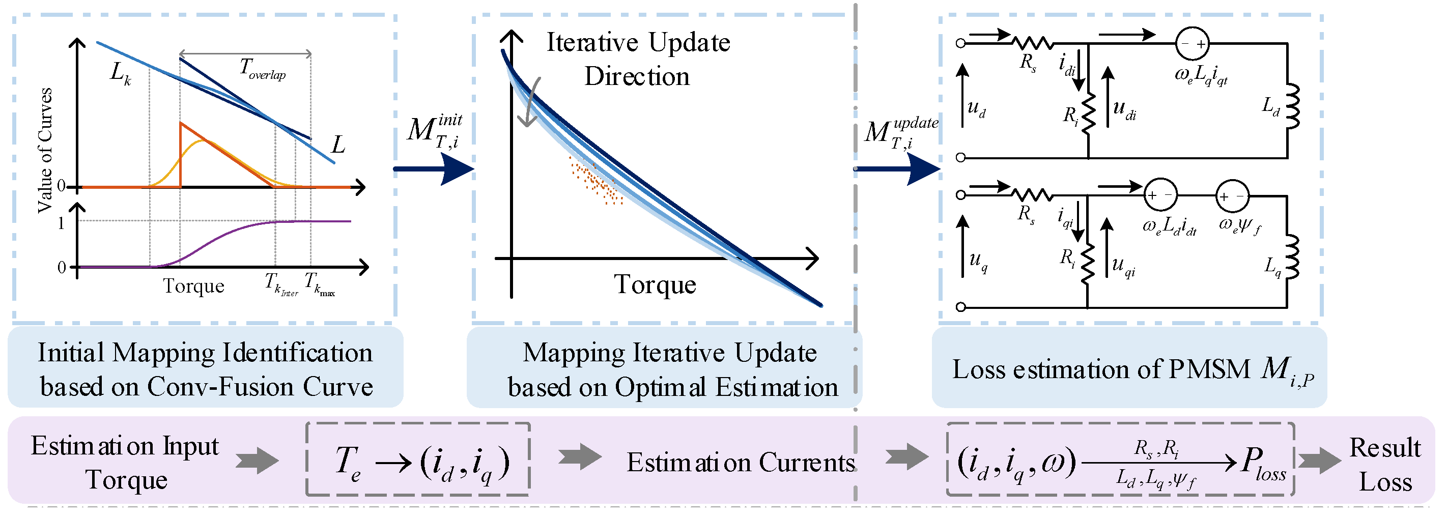
Figure 7 presents the implementation framework of the self-updating parametric PMSM loss estimation method. The blue section of Figure 7 indicates that the initial recognition mapping result is marked as , then the updated mapping result which marked as is obtained. Finally, by integrating with the PMSM loss model, the mapping relationship from torque to loss can be established. The purple section demonstrates the steps to be executed when performing loss estimation. When motor loss needs to be estimated, the control allocation unit takes torque and angular speed as inputs. First, the dq-axis current value is estimated by mapping , and then the motor loss is calculated by the current value using mapping . It is worth noting that the loss estimation and the recognition of the torque–current mapping do not follow the same execution cycle, loss estimation is only activated when performing control allocation calculations; whereas mapping updates are carried out at a lower priority and frequency.
| Algorithm 1 Mapping : Acquisition and Update |
|
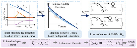
Figure 7.
Schematic diagram of the implementation of self-updating PMSM loss estimation.
4. Control Allocation with Line Search
The control allocation in a high-speed drive system can be abstracted as an optimization problem, with the reference torque of each motor as the output. The decision variable in this optimization problem is represented by the proportion of the reference torque of each motor in the total reference torque. A reasonable control allocation strategy should take into account both stability and economic performance. In the control allocation unit, the control of the total demanded torque and the torque output follow-up of a single motor do not need to be considered. Its stability focuses on ensuring that the torque allocated to each wheelset is within a reasonable range to avoid tire slipping caused by excessively high distribution coefficients [27]. Therefore, anti-slip constraints are introduced in the control allocation strategy to maintain system stability. The optimization objectives and optimization solutions are elaborated below.
4.1. Optimization Objectives and Constraints
The energy efficiency of the motor plays a critical role in the efficiency of the drive system. To enhance the economic performance of the system, comprehensive motor efficiency needs to be improved. Considering that the disparity in angular velocity among the motors is negligible, it is reasonable to approximate them as equal. Additionally, the sum of the reference torque of each motor is equal to the total reference torque. Thus the maximum comprehensive motor efficiency is the same as the minimum total motor losses.
The update interval for control allocation is denoted as . The present moment can be denoted as time t. Considering the time interval between the sampling time and the decision variables output, the current angular velocity of each motor, the train speed, and the total reference torque should be predicted with as the step size when constructing the optimization objectives. According to Equation (11), the prediction result can be expressed as follows.
where and represent angular velocity of motor i at time t and , and represent train speed at time t and , represents torque of motor i at time t, represents total reference torque at time , and represents the traction curve of the train. Hence, the energy-loss objective function can be represented as
where represents energy-loss objective function at time t, is the loss estimation of the i-th motor, is decision variable and presents torque distribution proportion of the i-th motor.
The penalty function method is used to handle constraints in the optimization problem. To maintain system stability, the slip rate of the wheelset should be within a limited range after the distributed torque acts on the system. The stability objective function at time t is designed as
where represents the predicted slip rate of motor i after the distributed torque at time acts on the system for duration. and represent angular velocity of motor i and train speed at time , which can be expressed as follows based on Equation (30).
is the penalty function, whose form is shown as
where represents the boundary constraint value of the slip rate. There is no penalty when the slip rate of the wheelset falls within the restricted range of .
Simultaneously, it is considered that the sum of the reference torques of each motor should be equivalent to the total reference torque. Consequently, a penalty term is introduced as shown as
As a result, the optimization objective at time t is shown below.
where , , represent the weight coefficients of the corresponding optimization item.
4.2. Optimization Solution with Line Search
During the operation of the train, the total reference torque and the angular velocity of each motor undergo changes, which means that the optimization objectives are time-various. The usual optimization strategy is to use the system state at a specific moment as a static optimization objective and to obtain the optimal solution through multiple iterations. Once the iteration termination condition is met, this optimal solution is used as the control output. The solution time of this method is long, and it is difficult to control the number of iterations, limiting the frequency of control allocation and making it unable to quickly adapt to changing operating conditions and system states.
The aim of this paper is to design an online control allocation strategy, thereby necessitating that the optimization solution method effectively adapts to real-time changes in operating conditions and minimizes computation time. As a result, an adaptive single-iteration gradient method that balances optimization effects with computational resource consumption is proposed. It executes only one iteration per control cycle to quickly adapt to new data and environmental changes. Additionally, this method prevents torque pulsation issues caused by fluctuations in control variables, by constraining multiple output results.
The gradient method iterates the solution vector in the negative gradient direction within the objective function to obtain the optimal solution [25]. In the drive system, the initial solution can be set as the point where the total torque is divided equally, specifically , . Because each component in solution is independent of each other, the gradient of the optimization function at position at time t can be calculated as the partial derivative of each component in the solution, which is expressed as follows.
where represents the i-th component of the solution . The partial derivatives are calculated using the difference method, as
where is the interval used in the difference method.
The solution is expressed as
where is called the step size at time t. When the value of the learning rate is too small, the convergence speed will be slow; when it is too large, oscillation will occur and convergence will be difficult. This paper designs an adaptive backtracking line search method based on the Armijo criterion [28,29] to obtain an appropriate step size.
The Armijo criterion can ensure that each iteration is sufficiently reduced. The chosen step size should satisfy
where is the search direction at and c is a constant, . The negative gradient direction is chosen as the search direction, so .
During the backtracking process, considering the impact of torque fluctuations and the variation of gradients under different operating conditions, a maximum step size limit is set as the initial state and initiates the descent search with as the decay factor, as . The initial state of the step size is set as follows.
where represents the i-th component of initial step size; K and are constants. When the total set torque is small, due to the decrease in the gradient of the objective function, to prevent the phenomenon of divergence caused by too high a learning rate, the learning rate is restricted. When the total set torque is large, the gradient of the objective function correspondingly increases. To avoid excessive fluctuations in the output, it is necessary to choose a smaller step size. However, to strictly control the time consumption of the backtracking line search, the numerical value is set as the forced exit condition. The search ends when the step size is less than . The specific implementation of control allocation can be seen in Algorithm 2.
| Algorithm 2 Control Allocation |
|
5. Experimental Procedure
In this section, the proposed control allocation strategy in this paper is verified by the HIL-based platform. As shown in Figure 8, the HIL-based platform consists of a traction control unit, a dSPACE real-time simulator (GmbH in Paderborn, Germany), signal conditioner, power source, and the host PC [30].
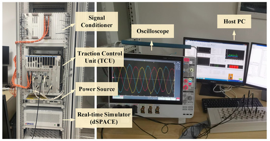
Figure 8.
Schematic diagram of hardware in the loop-based platform.
After building the multi-motor drive system model of the train, this section verifies the effectiveness of the strategy from two aspects: loss estimation and control allocation. The train parameters and the parameters of the PMSM are displayed in Table 1 and Table 2, respectively.

Table 1.
Train parameters.
Table 2.
Initial characteristic parameters of PMSM.
5.1. Performance for PMSM Loss Estimation
In this part, the train is set to be pulled from a state of rest to a steady velocity of 140 km/h. , , and the update period of the loss estimation model is 0.5s. This article utilizes the polynomial fitting method for the full-region data and the classic piecewise linear fitting method, where the average point of the endpoints of the two-region fitting results serves as the connection point. These methods are compared to evaluate the effectiveness of the proposed motor loss estimation method in this paper.
- A.
- Fitting performance.
Figure 9 displays the distribution of sampling data and the final fitting curve result during the initial identification stage of mapping . The figure illustrates that the distribution density of the sampling data is significantly higher at both ends of the torque range compared to the middle section, indicating a data imbalance phenomenon. Thus, the down-sampling method is employed to equalize the data, and the equalized data are utilized as verification data. The calculation of goodness of fit () and mean absolute percentage error (MAPE) of each method are shown as follows.
where is the verification data, is the corresponding value of loss estimation, is the mean of the verification data set, and m is the total number of data points in the data set. The results of calculating the above fitting indicators are shown in Table 3.
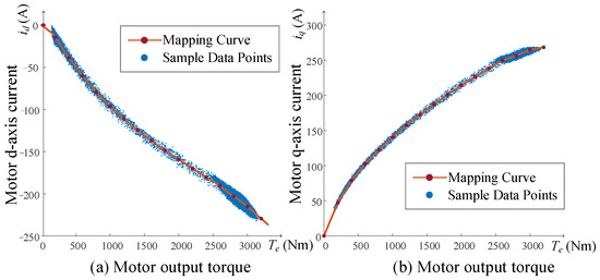
Figure 9.
Fitting result of mapping : (a) d-axis. (b) q-axis.
Table 3.
Fitting indicators of each method.
- B.
- Performance of loss estimation
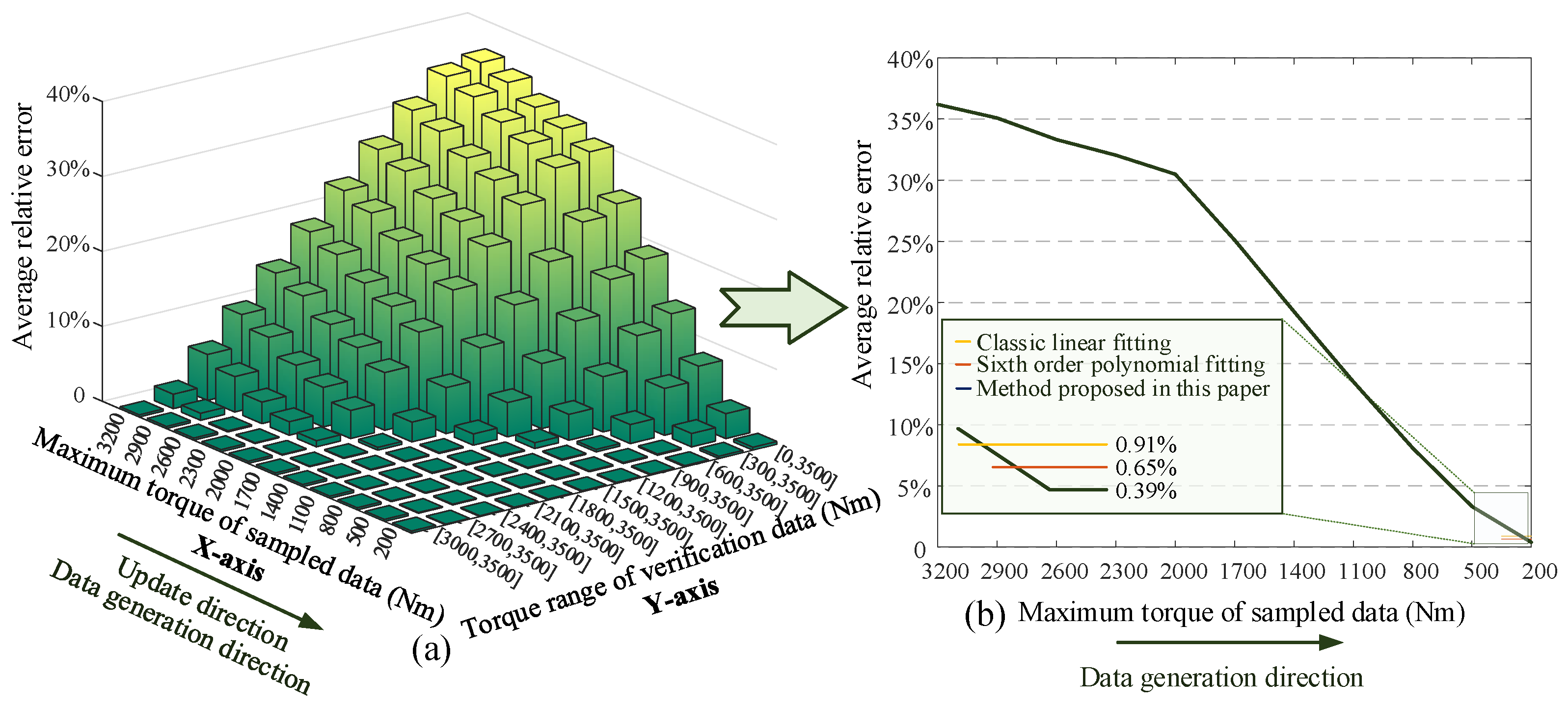
The average values of motor output torque, angular velocity, and loss data are selected from the system in its steady state. These averages are then compiled as a set of verification data. A series of such data sets is obtained under multiple torques, forming a comprehensive verification data set. The identification method of mapping proposed in this paper does not require waiting for the complete torque range data to be obtained. Instead, it optimizes the identification based on the sampled data, one by one. Figure 10 displays the average relative estimation error outcomes obtained from multiple identification results using verification data from various torque ranges.
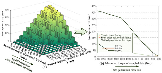
Figure 10.
Average relative error results of loss estimation under validation data for different torque ranges: (a) Multiple results under validation data for different torque ranges. (b) Multiple results under total torque ranges.
Throughout the train traction process, the torque corresponding to the collected sampling data gradually diminishes over time. The x-axis in Figure 10a represents the direction of the estimation model update, while the y-axis represents the division of verification data into multiple torque intervals. The average relative estimation error of losses is then calculated for the verification data in each interval. A certain updated estimation model yields accurate estimations for the verification data that exceed the range of torque values in the current sampling data. However, the estimation is ineffective for the torque range where sampling data has not been generated yet.
The data point corresponding to the y-axis mark in Figure 10a represents the computed errors for all verification data. The final results of all estimated models are displayed in Figure 10b. The x-axis mark 200 in Figure 10b represents that the maximum torque range for the current sampling data is 200 Nm. At this time, the data in the entire torque area have been generated, and the system enters the constant-speed operation state. Following that, the article compared the results of loss estimation using classic linear fitting and sixth-degree polynomial fitting. The proposed loss estimation method in this paper still demonstrates its superiority, as shown in Figure 10b.
5.2. Control Allocation Strategy Performance
The 16 power units in the train are evenly distributed among four groups. The motor parameters of two of the groups are displayed in Table 2, and the motor stator windings of the remaining two groups are augmented by 30%. To demonstrate the efficacy of the allocation strategy, various methods listed below are compared in terms of their control performance and economic performance during the traction process and constant-speed operation.
- The control allocation strategy proposed in this paper.The solution vector updates at a frequency of 1 kHz, meaning the distribution coefficients are updated every 0.001s.
- Torque average allocation.
- Classic gradient descent (GD).The torque distribution coefficients are used as the solution vector. By setting an appropriate learning rate, the solution vector is updated in the negative direction of the gradient. Each update of the solution vector constitutes one iteration. In the experiment, the number of iterations was set to 100, that is, the result of 100 updates of the solution vector was selected as the torque distribution coefficient.
- Particle swarm optimization (PSO).The torque distribution coefficients represent the positions of the particles, with each state of a particle representing a potential solution. Initially, particles are randomly distributed in the solution space and explore this space by adjusting their flight speed and direction, while recording the optimal solution. Each movement of a particle’s position is considered one iteration. The experiment was set to perform 100 iterations, with the best position selected as the output for the motor torque coefficients.
- Genetic algorithm (GA).The torque distribution coefficient of each motor is encoded as a “gene”, and the evolutionary process of selecting, crossing, and mutating to generate a new generation is an iterative process. In the experiment, the number of iterations was set to 100, that is, the motor torque distribution coefficient corresponding to the optimal population “gene” after the 100th generation was used as the output.
The torque average allocation method is employed as a control allocation strategy in trains currently. Iteration frequency means the rate at which an iteration process occurs within an optimization algorithm. Subsequently, 1 kHz and 10 kHz are employed as iteration frequencies in the latter two methods to facilitate comparison and validation.
- A.
- Iteration frequency 1 kHz
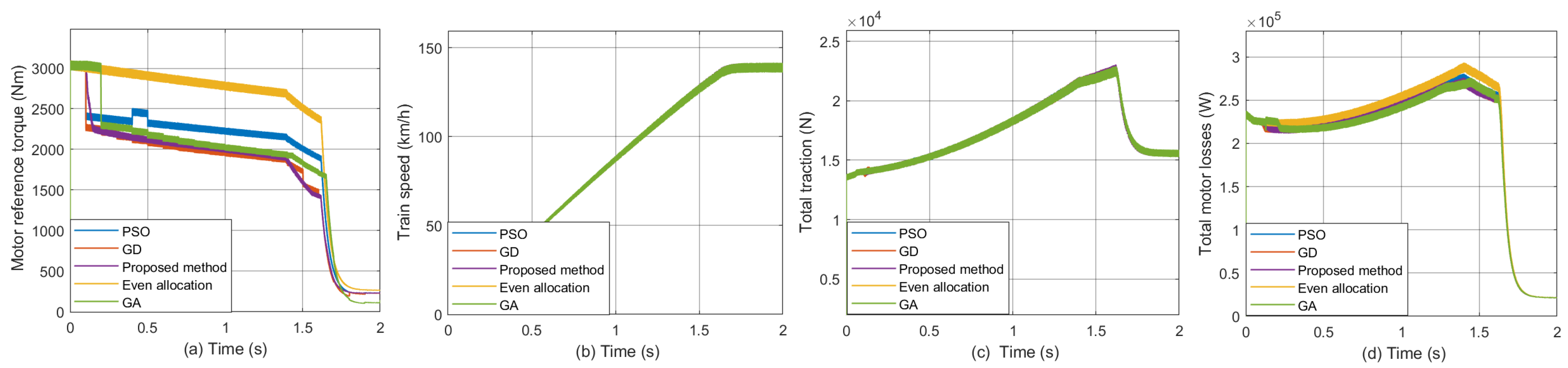
At an iteration frequency of 1 kHz, the control distribution coefficient is updated every 0.1s using the classic GD, PSO, and GA methods. Figure 11 illustrates the alterations in motor reference torque, total motor losses, train speed, and total train traction force when different methods are used in traction and constant speed conditions. The distribution coefficients of the four groups of motors in this process are depicted in Figure 12. Several conclusions can be drawn, as follows:
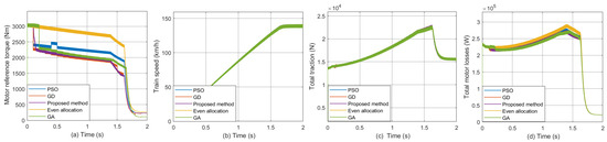
Figure 11.
Comparison of various methods under traction and constant speed when iteration frequency is 1 kHz: (a) Motor reference torque. (b) Train speed. (c) Train traction force. (d) Total motor losses.
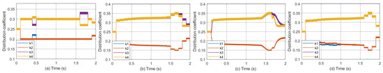
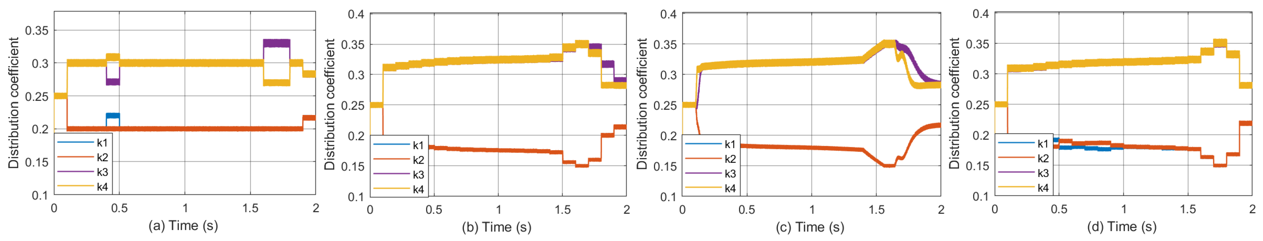
Figure 12.
Distribution coefficients of each method under traction and constant speed when iteration frequency is 1 kHz: (a) PSO. (b) GD. (c) Proposed Method. (d) GA.
- The optimization method results in a lower total loss of the motor under control allocation compared to the average allocation (see Figure 11d). The train speed and total traction force are nearly identical (see Figure 11b,c), indicating that the system maintains effective control and motion performance through control allocation.
- GD outperforms PSO and GA in terms of optimization effectiveness when the number of iterations is held constant (see Figure 12).
- Due to its inherent randomness, the results of GA may occasionally exhibit fluctuations (see Figure 12d).
- Since the classic GD, PSO, and GA methods require multiple iterations, the time interval for updating the distribution coefficient is lengthy. Additionally, the reference torque changes abruptly in response to rapid changes in the total demand torque. While using the strategy proposed in this paper, the distribution coefficient exhibits smooth changes and has minimal impact on the system.
- B.
- Iteration frequency 10 kHz
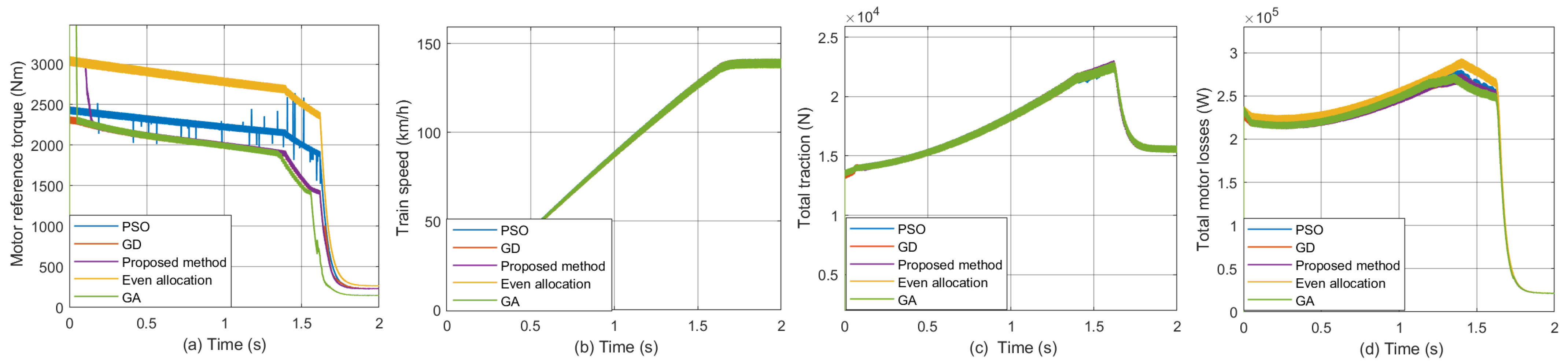
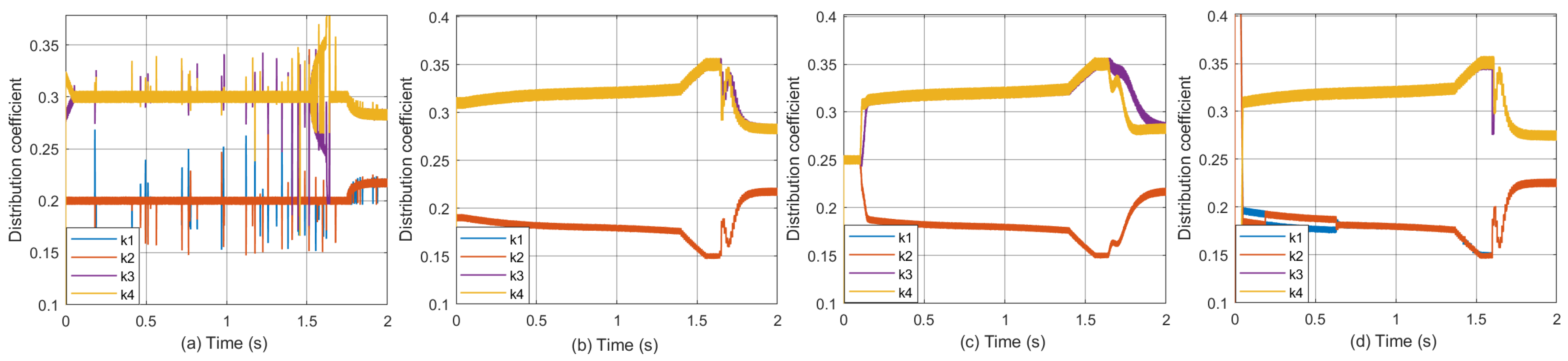
When the iteration frequency is 10 kHz, the update interval of the control distribution coefficient based on the classic GD, PSO, and GA is 0.01 s. As above, the comparative verification results in this case are shown in Figure 13 and Figure 14. Several conclusions can be drawn, as follows:
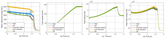
Figure 13.
Comparison of various methods under traction and constant speed when iteration frequency is 10 kHz: (a) Motor reference torque. (b) Train speed. (c) Train traction force. (d) Total motor losses.

Figure 14.
Distribution coefficients of each method under traction and constant speed when iteration frequency is 10 kHz: (a) PSO. (b) GD. (c) Proposed Method. (d) GA.
- Due to the shortened coefficient update time, the classic GD produces allocation results that are similar to the results obtained using the control allocation strategy proposed in this article. However, the classic GD requires significantly more computing resources compared to the latter, and the GA also has the same problem.
- The distribution coefficient in PSO exhibits numerous anomalies (see Figure 13a and Figure 14a). PSO is a prototypical algorithm for group optimization. Group optimization algorithms inherently possess a certain level of randomness, and excessively rapid update intervals can undermine system stability.
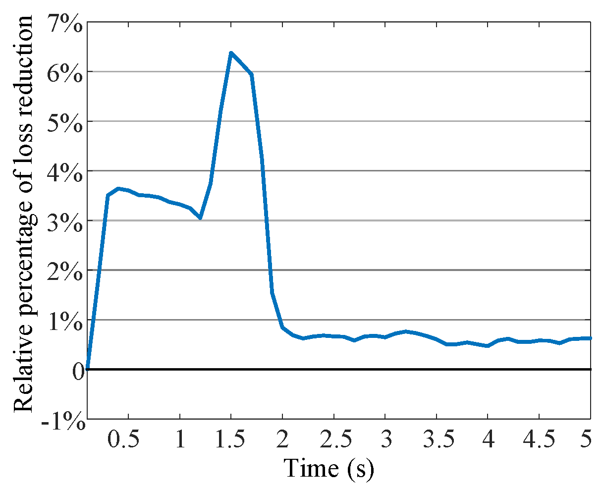
Based on the aforementioned analysis, it can be proved that the control allocation strategy proposed in this article outperforms the latter two optimization methods in terms of both stability and economic performance. Figure 15 displays the percentage by which the proposed control allocation strategy reduces loss relative to the average allocation method currently in use. During the traction state, there is a significant reduction in loss up to 6%.
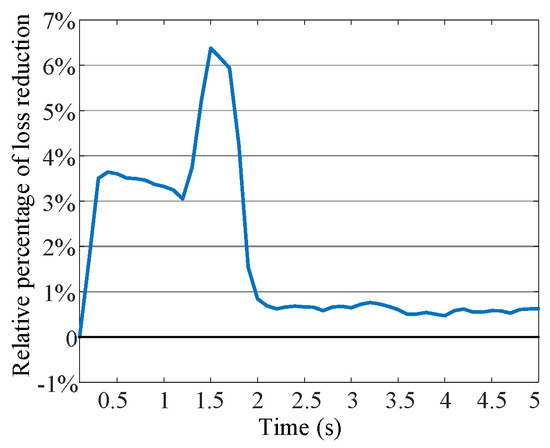
Figure 15.
Relative percentage of loss reduction of the proposed control allocation strategy.
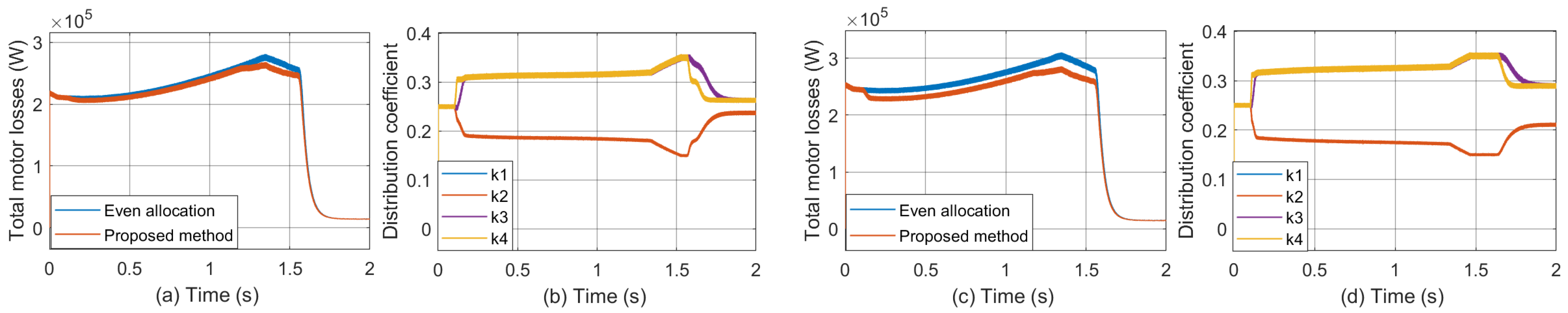
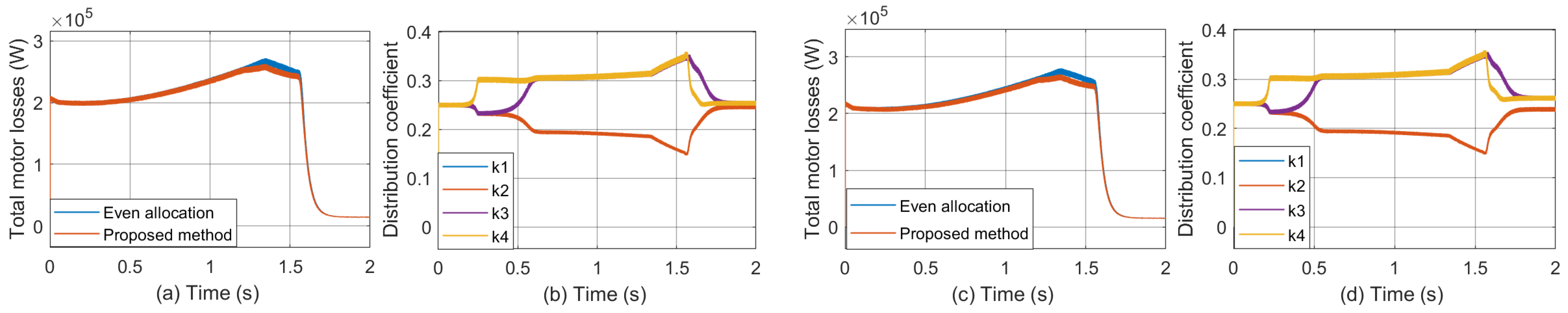
To further verify the system’s reproducibility, this paper validates the control allocation strategy under other conditions of changing motor parameters. Considering that the transverse and longitudinal axis inductances have a minimal impact on motor losses, we focused on the effects of changes in stator winding resistance and rotor flux linkage. Figure 16 shows the system’s total losses and torque distribution coefficients when the stator winding resistance of individual units increased by 10% and 50%. Figure 17 displays the total motor losses and torque distribution coefficients when the stator flux linkage of individual units decreased by 10% and 30%. Compared to the average allocation method, the method proposed in this paper significantly reduced the system’s total losses while maintaining the total traction force and train speed consistent with the scenarios shown in Figure 11 and Figure 13, proving that the system’s control performance was not affected.
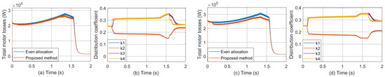
Figure 16.
Total motor losses and torque distribution coefficients following various changes in winding resistance: (a) Total motor losses with a 10% increase in winding resistance. (b) Torque distribution coefficients with a 10% increase in winding resistance. (c) Total motor losses with a 50% increase in winding resistance. (d) Torque distribution coefficients with a 50% increase in winding resistance.
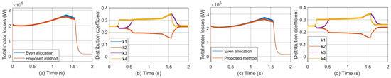
Figure 17.
Total motor losses and torque distribution coefficients following various changes in rotor flux linkage: (a) Total motor losses with a 10% reduction in rotor flux linkage. (b) Torque distribution coefficients with a 10% reduction in rotor flux linkage. (c) Total motor losses with a 30% reduction in rotor flux linkage. (d) Torque distribution coefficients with a 30% reduction in rotor flux linkage.
Table 4 shows the average total motor losses and steady state torque distribution coefficients under the average allocation method and the proposed control allocation methods within a simulation duration of 5 s, considering changes in various parameters. Analysis of the data in the table leads to the following conclusions:
Table 4.
Total motor losses and distribution coefficients under average allocation and the proposed method.
- Different types of parameters have varying levels of impact on the distribution results; the distribution is more sensitive to parameters that significantly affect motor losses.
- The larger the parameter changes, the more pronounced the differences among the motors become. Compared to the average allocation, the proposed method shows more significant energy-saving effects, and the differences in torque distribution coefficients among the motors are also more pronounced.
6. Conclusions
This paper focuses on the energy saving problems in the control allocation of multi-motor drive systems. To tackle the challenges in establishing correlation between motor parameters and the estimation loss and the torque fluctuation in real-time allocation, an online energy-saving control allocation strategy based on self-updating loss estimation is proposed. The significance of this paper can be outlined below:
- A self-updating PMSM loss estimation method based on dynamic torque–current mapping identification is proposed, which retains a direct correlation between motor loss and parameters, addressing the challenge of timely estimation of PMSM loss through various motor parameters.
- A dynamic optimization solution method based on line search in the control allocation process is proposed, which solves the distribution coefficients more stably, effectively mitigating the adverse effects such as torque shocks caused by fluctuations in the distribution coefficients.
- The results demonstrate that the strategy effectively enhances the energy efficiency of the multi-motor drive system while maintaining the original control performance of the system.
In the future, we will endeavor to further refine the proposed strategy by integrating real operational data into the existing train operation systems. This will facilitate the practical application of the strategy in engineering projects. Such enhancements are expected to improve the energy efficiency of train traction drive systems, thereby promoting the development of green railways.
Author Contributions
Methodology, Y.C., T.P. and J.G.; software, Y.X. and J.L.; validation, J.G.; writing—original draft preparation, Y.C. and J.L.; writing—review and editing, Y.X. and T.P. All authors have read and agreed to the published version of the manuscript.
Funding
This work was supported in part by the National Natural Science Foundation of China under Grants 62173350 and 62233012, by the Key Laboratory of Energy Saving Control and Safety Monitoring for Rail Transportation under Grant 2017TP1002, by the Fundamental Research Funds for the Central Universities of Central South University under Grant 2023ZZTS0963.
Data Availability Statement
Data are contained within the article.
Conflicts of Interest
The authors declare no conflicts of interest.
References
- El Alaoui, H.; Bazzi, A.; El Hafdaoui, H.; Khallaayoun, A.; Lghoul, R. Sustainable railways for Morocco: A comprehensive energy and environmental assessment. J. Umm-Qura Univ. Eng. Archit. 2023, 14, 271–283. [Google Scholar] [CrossRef]
- Yu, X.; Lin, C.; Tian, Y.; Zhao, M.; Liu, H.; Xie, P.; Zhang, J. Real-time and hierarchical energy management-control framework for electric vehicles with dual-motor powertrain system. Energy 2023, 272, 127112. [Google Scholar] [CrossRef]
- Wang, Z.; Zhou, J.; Rizzoni, G. A review of architectures and control strategies of dual-motor coupling powertrain systems for battery electric vehicles. Renew. Sustain. Energy Rev. 2022, 162, 112455. [Google Scholar] [CrossRef]
- Sorniotti, A.; Holdstock, T.; Everitt, M.; Fracchia, M.; Viotto, F.; Cavallino, C.; Bertolotto, S. A novel clutchless multiple-speed transmission for electric axles. Int. J. Powertrains 2013, 2, 103–131. [Google Scholar] [CrossRef]
- Hu, J.; Zheng, L.; Jia, M.; Zhang, Y.; Pang, T. Optimization and Model Validation of Operation Control Strategies for a Novel Dual-Motor Coupling-Propulsion Pure Electric Vehicle. Energies 2018, 11, 754. [Google Scholar] [CrossRef]
- Wang, W.; Shi, J.; Zhang, Z.; Lin, C. Optimization of a dual-motor coupled powertrain energy management strategy for a battery electric bus. Energy Procedia 2018, 145, 20–25. [Google Scholar] [CrossRef]
- Zhang, C.; Zhang, S.; Han, G.; Liu, H. Power management comparison for a dual-motor-propulsion system used in a battery electric bus. IEEE Trans. Ind. Electron. 2017, 64, 3873–3882. [Google Scholar] [CrossRef]
- Yuan, X.; Wang, J. Torque distribution strategy for a front-and rear-wheel-driven electric vehicle. IEEE Trans. Veh. Technol. 2012, 61, 3365–3374. [Google Scholar] [CrossRef]
- Yu, Z.; Zhang, L.; Xiong, L. Optimized Torque Distribution Control to Achieve Higher Fuel Economy of Electric Vehicle with Four In-Wheel Motors. J. Tongji Univ. (Nat. Sci.) 2005, 33, 1355–1361. (In Chinese) [Google Scholar]
- Gu, J.; Ouyang, M.; Lu, D.; Li, J.; Lu, L. Energy efficiency optimization of electric vehicle driven by in-wheel motors. Int. J. Automot. Technol. 2013, 14, 763–772. [Google Scholar] [CrossRef]
- Song, Z.; Hofmann, H.; Li, J.; Wang, Y.; Lu, D.; Ouyang, M.; Du, J. Torque distribution strategy for multi-PMSM applications and optimal acceleration control for four-wheel-drive electric vehicles. J. Dyn. Syst. Meas. Control. 2020, 142, 021001. [Google Scholar] [CrossRef]
- Dianov, A.; Ballard, B.; Blundell, M.; Kanarachos, S.; Innocente, M.S. A Non-Convex Control Allocation Strategy as Energy-Efficient Torque Distributors for On-Road and Off-Road Vehicles. Control Eng. Pract. 2020, 95, 104256. [Google Scholar]
- Torinsson, J.; Jonasson, M.; Yang, D.; Jacobson, B. Energy reduction by power loss minimisation through wheel torque allocation in electric vehicles: A simulation-based approach. Veh. Syst. Dyn. 2022, 60, 1488–1511. [Google Scholar] [CrossRef]
- He, S.; Fan, X.; Wang, Q.; Chen, X.; Zhu, S. Review on torque distribution scheme of four-wheel in-wheel motor electric vehicle. Machines 2022, 10, 619. [Google Scholar] [CrossRef]
- Parra, A.; Tavernini, D.; Gruber, P.; Sorniotti, A.; Zubizarreta, A.; Pérez, J. On Nonlinear Model Predictive Control for Energy-Efficient Torque-Vectoring. IEEE Trans. Veh. Technol. 2021, 70, 173–188. [Google Scholar] [CrossRef]
- Gao, B.; Yan, Y.; Chu, H.; Chen, H.; Xu, N. Torque allocation of four-wheel drive EVs considering tire slip energy. Sci. China Inf. Sci. 2022, 65, 122202. [Google Scholar] [CrossRef]
- Liu, J.; Wang, Z.; Hou, Y.; Qu, C.; Hong, J.; Lin, N. Data-driven energy management and velocity prediction for four-wheel-independent-driving electric vehicles. ETransportation 2021, 9, 100119. [Google Scholar] [CrossRef]
- Wei, H.; Ai, Q.; Zhao, W.; Zhang, Y. Modelling and experimental validation of an EV torque distribution strategy towards active safety and energy efficiency. Energy 2022, 239, 121953. [Google Scholar] [CrossRef]
- Wei, H.; Fan, L.; Ai, Q.; Zhao, W.; Huang, T.; Zhang, Y. Optimal energy allocation strategy for electric vehicles based on the real-time model predictive control technology. Sustain. Energy Technol. Assess. 2022, 50, 101797. [Google Scholar] [CrossRef]
- Wang, J.; Gao, S.; Wang, K.; Wang, Y.; Wang, Q. Wheel torque distribution optimization of four-wheel independent-drive electric vehicle for energy efficient driving. Control Eng. Pract. 2021, 110, 104779. [Google Scholar] [CrossRef]
- Jiang, Y.; Meng, H.; Chen, G.; Xu, X.; Zhang, L.; Xu, H. Differential-steering based path tracking control and energy-saving torque distribution strategy of 6WID unmanned ground vehicle. Energy 2022, 254, 124209. [Google Scholar] [CrossRef]
- Gui, W.; Gao, J.; Yang, C.; Peng, T.; Yang, C.; Han, Y. Optimized FCS-MPCC based on disturbance feedback rejection for IPMSMs under demagnetization fault in high-speed trains. Control Eng. Pract. 2023, 141, 105670. [Google Scholar] [CrossRef]
- Liang, J.; Feng, J.; Fang, Z.; Lu, Y.; Yin, G.; Mao, X.; Wu, J.; Wang, F. An Energy-Oriented Torque-Vector Control Framework for Distributed Drive Electric Vehicles. IEEE Trans. Transp. Electrif. 2023, 9, 4014–4031. [Google Scholar] [CrossRef]
- Abbasimoshaei, A.; Chinnakkonda Ravi, A.K.; Kern, T.A. Development of a new control system for a rehabilitation robot using electrical impedance tomography and artificial intelligence. Biomimetics 2023, 8, 420. [Google Scholar] [CrossRef] [PubMed]
- Ruder, S. An overview of gradient descent optimization algorithms. arXiv 2016, arXiv:1609.04747. [Google Scholar]
- Khodarahmi, M.; Maihami, V. A review on Kalman filter models. Arch. Comput. Methods Eng. 2023, 30, 727–747. [Google Scholar] [CrossRef]
- Uyulan, C.; Gokasan, M.; Bogosyan, S. Re-adhesion control strategy based on the optimal slip velocity seeking method. J. Mod. Transp. 2018, 26, 36–48. [Google Scholar] [CrossRef]
- Quiroz, E.; Papa, E.; Quispe, E.; Oliveira, P. Steepest descent method with a generalized Armijo search for quasiconvex functions on Riemannian manifolds. J. Math. Anal. Appl. 2008, 341, 467–477. [Google Scholar] [CrossRef]
- Wang, J.; Zhang, B.; Sun, Z.; Hao, W.; Sun, Q. A novel conjugate gradient method with generalized Armijo search for efficient training of feedforward neural networks. Neurocomputing 2018, 275, 308–316. [Google Scholar] [CrossRef]
- Yin, S.; Peng, T.; Chen, Y.; Yang, C.; Yang, C.; Gui, W.; Liu, L. Variable domain hybrid decision-based friction optimization control for train multi-wheelsets. Tribol. Int. 2024, 195, 109638. [Google Scholar] [CrossRef]


Disclaimer/Publisher’s Note: The statements, opinions and data contained in all publications are solely those of the individual author(s) and contributor(s) and not of MDPI and/or the editor(s). MDPI and/or the editor(s) disclaim responsibility for any injury to people or property resulting from any ideas, methods, instructions or products referred to in the content. |
© 2024 by the authors. Licensee MDPI, Basel, Switzerland. This article is an open access article distributed under the terms and conditions of the Creative Commons Attribution (CC BY) license (https://creativecommons.org/licenses/by/4.0/).