

An Online Energy-Saving Control Allocation Strategy Based on Self-Updating Loss Estimation for Multi-Motor Drive Systems

Abstract
1. Introduction
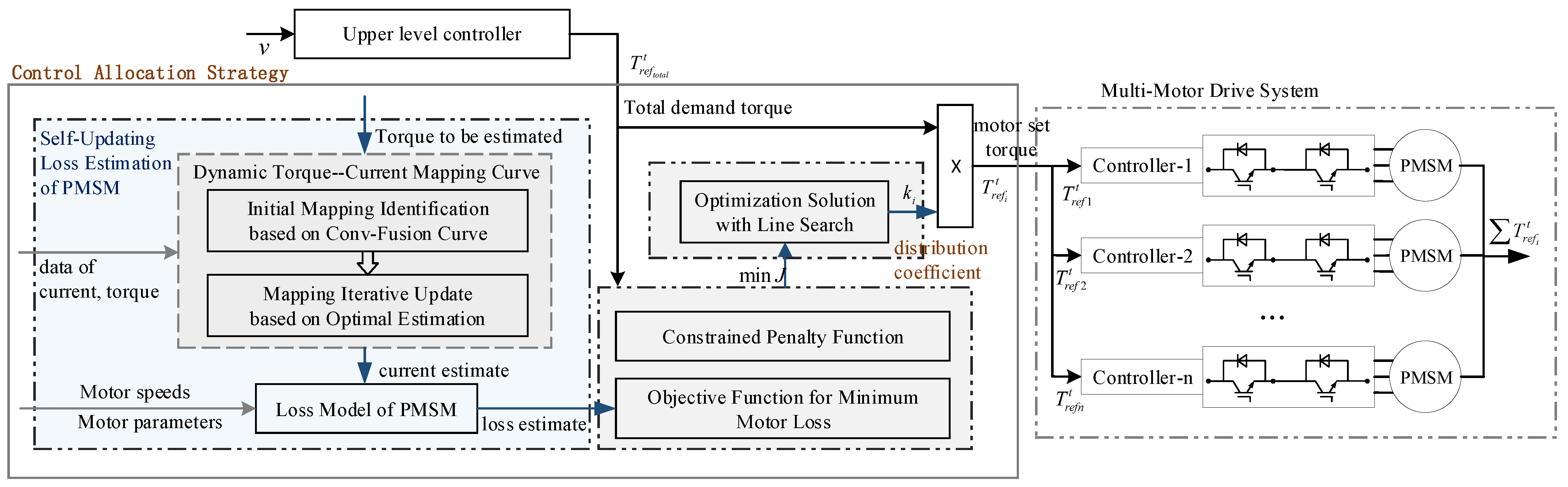
- A self-updating PMSM loss estimation method based on dynamic torque–current mapping is proposed. The torque–current mapping is initially identified based on the conv-fusion curve, and is iteratively updated based on optimal estimation. This method retains a direct correlation between motor loss and parameters and enjoys extensive flexibility in motor control methods, effectively addressing the challenge of promptly estimating PMSM loss through various motor parameters.
- A novel online control allocation method based on line search is proposed. This method leverages the descent method, incorporating the Armijo criterion and backtracking to determine an optimal step size, and an initial search value of it is designed to regulate torque changes. With these designs, the method can effectively reduce total motor loss and mitigate the impact of variations in distribution coefficients, and thus maintains real-time performance.
2. Drive System Composition and Modeling
2.1. PMSM Modeling Considering Iron Loss
2.2. Drive System Modeling
3. Self-Updating Loss Estimation of PMSM
3.1. Initial Mapping Identification Based on Conv-Fusion Curve
3.2. Mapping Iterative Update Based on Optimal Estimation
3.3. Loss Estimation of PMSM
| Algorithm 1 Mapping : Acquisition and Update |
|
4. Control Allocation with Line Search
4.1. Optimization Objectives and Constraints
4.2. Optimization Solution with Line Search
| Algorithm 2 Control Allocation |
|
5. Experimental Procedure
5.1. Performance for PMSM Loss Estimation
- A.
- Fitting performance.
- B.
- Performance of loss estimation
5.2. Control Allocation Strategy Performance
- The control allocation strategy proposed in this paper.The solution vector updates at a frequency of 1 kHz, meaning the distribution coefficients are updated every 0.001s.
- Torque average allocation.
- Classic gradient descent (GD).The torque distribution coefficients are used as the solution vector. By setting an appropriate learning rate, the solution vector is updated in the negative direction of the gradient. Each update of the solution vector constitutes one iteration. In the experiment, the number of iterations was set to 100, that is, the result of 100 updates of the solution vector was selected as the torque distribution coefficient.
- Particle swarm optimization (PSO).The torque distribution coefficients represent the positions of the particles, with each state of a particle representing a potential solution. Initially, particles are randomly distributed in the solution space and explore this space by adjusting their flight speed and direction, while recording the optimal solution. Each movement of a particle’s position is considered one iteration. The experiment was set to perform 100 iterations, with the best position selected as the output for the motor torque coefficients.
- Genetic algorithm (GA).The torque distribution coefficient of each motor is encoded as a “gene”, and the evolutionary process of selecting, crossing, and mutating to generate a new generation is an iterative process. In the experiment, the number of iterations was set to 100, that is, the motor torque distribution coefficient corresponding to the optimal population “gene” after the 100th generation was used as the output.
- A.
- Iteration frequency 1 kHz
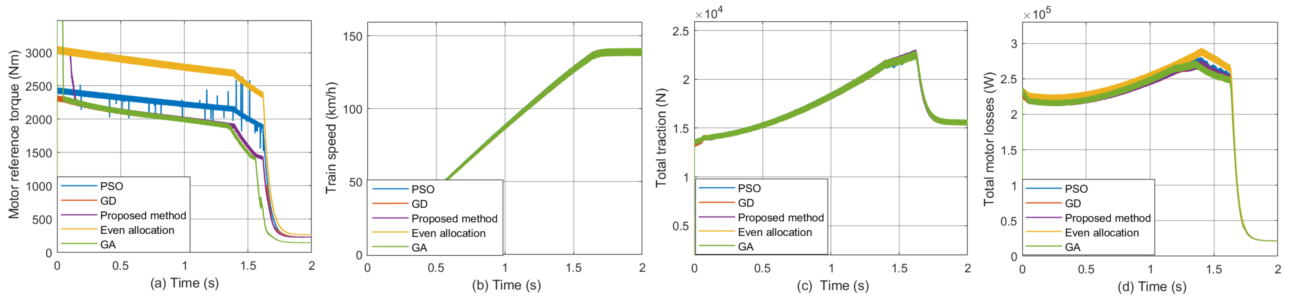
- The optimization method results in a lower total loss of the motor under control allocation compared to the average allocation (see Figure 11d). The train speed and total traction force are nearly identical (see Figure 11b,c), indicating that the system maintains effective control and motion performance through control allocation.
- GD outperforms PSO and GA in terms of optimization effectiveness when the number of iterations is held constant (see Figure 12).
- Due to its inherent randomness, the results of GA may occasionally exhibit fluctuations (see Figure 12d).
- Since the classic GD, PSO, and GA methods require multiple iterations, the time interval for updating the distribution coefficient is lengthy. Additionally, the reference torque changes abruptly in response to rapid changes in the total demand torque. While using the strategy proposed in this paper, the distribution coefficient exhibits smooth changes and has minimal impact on the system.
- B.
- Iteration frequency 10 kHz
- Due to the shortened coefficient update time, the classic GD produces allocation results that are similar to the results obtained using the control allocation strategy proposed in this article. However, the classic GD requires significantly more computing resources compared to the latter, and the GA also has the same problem.
- The distribution coefficient in PSO exhibits numerous anomalies (see Figure 13a and Figure 14a). PSO is a prototypical algorithm for group optimization. Group optimization algorithms inherently possess a certain level of randomness, and excessively rapid update intervals can undermine system stability.
- Different types of parameters have varying levels of impact on the distribution results; the distribution is more sensitive to parameters that significantly affect motor losses.
- The larger the parameter changes, the more pronounced the differences among the motors become. Compared to the average allocation, the proposed method shows more significant energy-saving effects, and the differences in torque distribution coefficients among the motors are also more pronounced.
6. Conclusions
- A self-updating PMSM loss estimation method based on dynamic torque–current mapping identification is proposed, which retains a direct correlation between motor loss and parameters, addressing the challenge of timely estimation of PMSM loss through various motor parameters.
- A dynamic optimization solution method based on line search in the control allocation process is proposed, which solves the distribution coefficients more stably, effectively mitigating the adverse effects such as torque shocks caused by fluctuations in the distribution coefficients.
- The results demonstrate that the strategy effectively enhances the energy efficiency of the multi-motor drive system while maintaining the original control performance of the system.
Author Contributions
Funding
Data Availability Statement
Conflicts of Interest
References
- El Alaoui, H.; Bazzi, A.; El Hafdaoui, H.; Khallaayoun, A.; Lghoul, R. Sustainable railways for Morocco: A comprehensive energy and environmental assessment. J. Umm-Qura Univ. Eng. Archit. 2023, 14, 271–283. [Google Scholar] [CrossRef]
- Yu, X.; Lin, C.; Tian, Y.; Zhao, M.; Liu, H.; Xie, P.; Zhang, J. Real-time and hierarchical energy management-control framework for electric vehicles with dual-motor powertrain system. Energy 2023, 272, 127112. [Google Scholar] [CrossRef]
- Wang, Z.; Zhou, J.; Rizzoni, G. A review of architectures and control strategies of dual-motor coupling powertrain systems for battery electric vehicles. Renew. Sustain. Energy Rev. 2022, 162, 112455. [Google Scholar] [CrossRef]
- Sorniotti, A.; Holdstock, T.; Everitt, M.; Fracchia, M.; Viotto, F.; Cavallino, C.; Bertolotto, S. A novel clutchless multiple-speed transmission for electric axles. Int. J. Powertrains 2013, 2, 103–131. [Google Scholar] [CrossRef]
- Hu, J.; Zheng, L.; Jia, M.; Zhang, Y.; Pang, T. Optimization and Model Validation of Operation Control Strategies for a Novel Dual-Motor Coupling-Propulsion Pure Electric Vehicle. Energies 2018, 11, 754. [Google Scholar] [CrossRef]
- Wang, W.; Shi, J.; Zhang, Z.; Lin, C. Optimization of a dual-motor coupled powertrain energy management strategy for a battery electric bus. Energy Procedia 2018, 145, 20–25. [Google Scholar] [CrossRef]
- Zhang, C.; Zhang, S.; Han, G.; Liu, H. Power management comparison for a dual-motor-propulsion system used in a battery electric bus. IEEE Trans. Ind. Electron. 2017, 64, 3873–3882. [Google Scholar] [CrossRef]
- Yuan, X.; Wang, J. Torque distribution strategy for a front-and rear-wheel-driven electric vehicle. IEEE Trans. Veh. Technol. 2012, 61, 3365–3374. [Google Scholar] [CrossRef]
- Yu, Z.; Zhang, L.; Xiong, L. Optimized Torque Distribution Control to Achieve Higher Fuel Economy of Electric Vehicle with Four In-Wheel Motors. J. Tongji Univ. (Nat. Sci.) 2005, 33, 1355–1361. (In Chinese) [Google Scholar]
- Gu, J.; Ouyang, M.; Lu, D.; Li, J.; Lu, L. Energy efficiency optimization of electric vehicle driven by in-wheel motors. Int. J. Automot. Technol. 2013, 14, 763–772. [Google Scholar] [CrossRef]
- Song, Z.; Hofmann, H.; Li, J.; Wang, Y.; Lu, D.; Ouyang, M.; Du, J. Torque distribution strategy for multi-PMSM applications and optimal acceleration control for four-wheel-drive electric vehicles. J. Dyn. Syst. Meas. Control. 2020, 142, 021001. [Google Scholar] [CrossRef]
- Dianov, A.; Ballard, B.; Blundell, M.; Kanarachos, S.; Innocente, M.S. A Non-Convex Control Allocation Strategy as Energy-Efficient Torque Distributors for On-Road and Off-Road Vehicles. Control Eng. Pract. 2020, 95, 104256. [Google Scholar]
- Torinsson, J.; Jonasson, M.; Yang, D.; Jacobson, B. Energy reduction by power loss minimisation through wheel torque allocation in electric vehicles: A simulation-based approach. Veh. Syst. Dyn. 2022, 60, 1488–1511. [Google Scholar] [CrossRef]
- He, S.; Fan, X.; Wang, Q.; Chen, X.; Zhu, S. Review on torque distribution scheme of four-wheel in-wheel motor electric vehicle. Machines 2022, 10, 619. [Google Scholar] [CrossRef]
- Parra, A.; Tavernini, D.; Gruber, P.; Sorniotti, A.; Zubizarreta, A.; Pérez, J. On Nonlinear Model Predictive Control for Energy-Efficient Torque-Vectoring. IEEE Trans. Veh. Technol. 2021, 70, 173–188. [Google Scholar] [CrossRef]
- Gao, B.; Yan, Y.; Chu, H.; Chen, H.; Xu, N. Torque allocation of four-wheel drive EVs considering tire slip energy. Sci. China Inf. Sci. 2022, 65, 122202. [Google Scholar] [CrossRef]
- Liu, J.; Wang, Z.; Hou, Y.; Qu, C.; Hong, J.; Lin, N. Data-driven energy management and velocity prediction for four-wheel-independent-driving electric vehicles. ETransportation 2021, 9, 100119. [Google Scholar] [CrossRef]
- Wei, H.; Ai, Q.; Zhao, W.; Zhang, Y. Modelling and experimental validation of an EV torque distribution strategy towards active safety and energy efficiency. Energy 2022, 239, 121953. [Google Scholar] [CrossRef]
- Wei, H.; Fan, L.; Ai, Q.; Zhao, W.; Huang, T.; Zhang, Y. Optimal energy allocation strategy for electric vehicles based on the real-time model predictive control technology. Sustain. Energy Technol. Assess. 2022, 50, 101797. [Google Scholar] [CrossRef]
- Wang, J.; Gao, S.; Wang, K.; Wang, Y.; Wang, Q. Wheel torque distribution optimization of four-wheel independent-drive electric vehicle for energy efficient driving. Control Eng. Pract. 2021, 110, 104779. [Google Scholar] [CrossRef]
- Jiang, Y.; Meng, H.; Chen, G.; Xu, X.; Zhang, L.; Xu, H. Differential-steering based path tracking control and energy-saving torque distribution strategy of 6WID unmanned ground vehicle. Energy 2022, 254, 124209. [Google Scholar] [CrossRef]
- Gui, W.; Gao, J.; Yang, C.; Peng, T.; Yang, C.; Han, Y. Optimized FCS-MPCC based on disturbance feedback rejection for IPMSMs under demagnetization fault in high-speed trains. Control Eng. Pract. 2023, 141, 105670. [Google Scholar] [CrossRef]
- Liang, J.; Feng, J.; Fang, Z.; Lu, Y.; Yin, G.; Mao, X.; Wu, J.; Wang, F. An Energy-Oriented Torque-Vector Control Framework for Distributed Drive Electric Vehicles. IEEE Trans. Transp. Electrif. 2023, 9, 4014–4031. [Google Scholar] [CrossRef]
- Abbasimoshaei, A.; Chinnakkonda Ravi, A.K.; Kern, T.A. Development of a new control system for a rehabilitation robot using electrical impedance tomography and artificial intelligence. Biomimetics 2023, 8, 420. [Google Scholar] [CrossRef] [PubMed]
- Ruder, S. An overview of gradient descent optimization algorithms. arXiv 2016, arXiv:1609.04747. [Google Scholar]
- Khodarahmi, M.; Maihami, V. A review on Kalman filter models. Arch. Comput. Methods Eng. 2023, 30, 727–747. [Google Scholar] [CrossRef]
- Uyulan, C.; Gokasan, M.; Bogosyan, S. Re-adhesion control strategy based on the optimal slip velocity seeking method. J. Mod. Transp. 2018, 26, 36–48. [Google Scholar] [CrossRef]
- Quiroz, E.; Papa, E.; Quispe, E.; Oliveira, P. Steepest descent method with a generalized Armijo search for quasiconvex functions on Riemannian manifolds. J. Math. Anal. Appl. 2008, 341, 467–477. [Google Scholar] [CrossRef]
- Wang, J.; Zhang, B.; Sun, Z.; Hao, W.; Sun, Q. A novel conjugate gradient method with generalized Armijo search for efficient training of feedforward neural networks. Neurocomputing 2018, 275, 308–316. [Google Scholar] [CrossRef]
- Yin, S.; Peng, T.; Chen, Y.; Yang, C.; Yang, C.; Gui, W.; Liu, L. Variable domain hybrid decision-based friction optimization control for train multi-wheelsets. Tribol. Int. 2024, 195, 109638. [Google Scholar] [CrossRef]


| Symbol | Meaning | Value |
|---|---|---|
| Positive pressure of module | 11,500 N | |
| M | Train mass | 408 t |
| r | Wheel radius | 0.4375 m |
| J | Equivalent rotational inertia | 16.6 kg·m2 |
| Transmission efficiency of gear | 0.97 | |
| a | Transmission ratio of gear | 2.788 |
| Adhesion coefficient curve |
| Symbol | Meaning | Value |
|---|---|---|
| Inductance of the d-axis | 3.7 mH | |
| Inductance of the q-axis | 9.6 mH | |
| Resistance of stator | 0.07 | |
| Equivalent iron loss resistance | 1000 | |
| Flux linkage of permanent magnet | 0.625 Wb | |
| Number of poles | 4 |
| Methods | of | MAPE of | of | MAPE of |
|---|---|---|---|---|
| Conv-fusion curve | 0.9999 | 0.0058 | 0.9999 | 0.0034 |
| Fifth-degree polynomial | 0.9995 | 0.0130 | 0.9996 | 0.0058 |
| Sixth-degree polynomial | 0.9995 | 0.0143 | 0.9997 | 0.0062 |
| Classic piecewise linear fitting | 0.9997 | 0.0125 | 0.9999 | 0.0047 |
| Parameter Settings | Losses (Average Allocation) | Losses (Proposed Method) | Percentage of Loss Reduction | Distribution Coefficient |
|---|---|---|---|---|
| increase by 10% | 83,968 W | 82,214 W | 2.09% | 0.2629, 0.2629, 0.2371, 0.2371 |
| increase by 30% | 88,237 W | 85,074 W | 3.58% | 0.2748, 0.2748, 0.2252, 0.2252 |
| increase by 50% | 93,943 W | 88,754 W | 5.52% | 0.2893, 0.2893, 0.2107, 0.2107 |
| reduce by 10% | 81,087 W | 80,373 W | 0.88% | 0.2538, 0.2538, 0.2462, 0.2462 |
| reduce by 30% | 84,355 W | 83,302 W | 1.25% | 0.2613, 0.2613, 0.2387, 0.2387 |
Disclaimer/Publisher’s Note: The statements, opinions and data contained in all publications are solely those of the individual author(s) and contributor(s) and not of MDPI and/or the editor(s). MDPI and/or the editor(s) disclaim responsibility for any injury to people or property resulting from any ideas, methods, instructions or products referred to in the content. |
© 2024 by the authors. Licensee MDPI, Basel, Switzerland. This article is an open access article distributed under the terms and conditions of the Creative Commons Attribution (CC BY) license (https://creativecommons.org/licenses/by/4.0/).
Share and Cite
Chen, Y.; Peng, T.; Xu, Y.; Luo, J.; Gao, J. An Online Energy-Saving Control Allocation Strategy Based on Self-Updating Loss Estimation for Multi-Motor Drive Systems. Processes 2024, 12, 1072. https://doi.org/10.3390/pr12061072
Chen Y, Peng T, Xu Y, Luo J, Gao J. An Online Energy-Saving Control Allocation Strategy Based on Self-Updating Loss Estimation for Multi-Motor Drive Systems. Processes. 2024; 12(6):1072. https://doi.org/10.3390/pr12061072
Chicago/Turabian StyleChen, Yujie, Tao Peng, Yansong Xu, Junze Luo, and Jinqiu Gao. 2024. "An Online Energy-Saving Control Allocation Strategy Based on Self-Updating Loss Estimation for Multi-Motor Drive Systems" Processes 12, no. 6: 1072. https://doi.org/10.3390/pr12061072
APA StyleChen, Y., Peng, T., Xu, Y., Luo, J., & Gao, J. (2024). An Online Energy-Saving Control Allocation Strategy Based on Self-Updating Loss Estimation for Multi-Motor Drive Systems. Processes, 12(6), 1072. https://doi.org/10.3390/pr12061072