

A Predictive Model for Wellbore Temperature in High-Sulfur Gas Wells Incorporating Sulfur Deposition


Abstract
1. Introduction
2. Methodology
2.1. PPP Models
2.1.1. Deviation Coefficient
2.1.2. Viscosity
2.1.3. Thermal Conductivity Coefficient
2.2. WTD Model
2.2.1. Equation of Heat Conduction
2.2.2. Transient Temperature Model
- (1)
- The transmission of heat from high-temperature gas to the sulfur layer occurs through thermal convection.
- (2)
- Heat transfer in the sulfur layer, tubing, casing, and cement takes place through heat conduction.
- (3)
- The heat transfer in the annulus is characterized by convection and radiation.
2.3. Wellbore Pressure Model
2.4. Sulfur Solubility Model
2.5. Initial Conditions and Boundary Conditions
2.5.1. Initial Conditions
2.5.2. Boundary Conditions
2.6. Numerical Methods
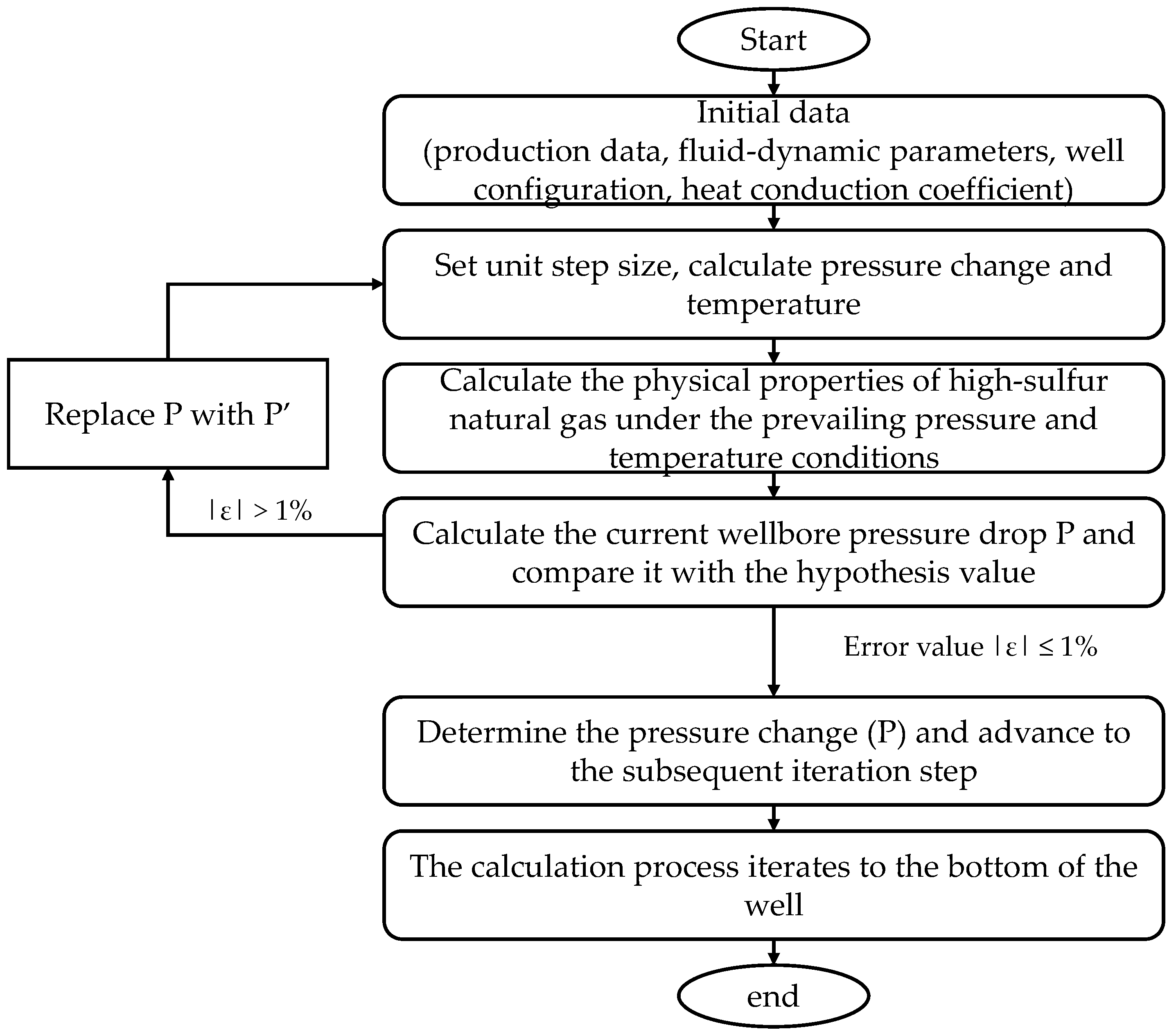
2.7. The Calculation Process
- (1)
- Initiate the program and input the initial parameters, which encompass well structure data, production performance data, physical property data, and the heat transfer coefficient.
- (2)
- Spatial and temporal discretization of the simulation domain is determined based on the depth and radial orientation of the well.
- (3)
- Calculate the initial temperature, pressure, and PPPs according to Section 2.1, Section 2.4 and Section 2.5.
- (4)
- At one time step, the pressure field distribution is first calculated. The pressure is calculated in stages from the wellhead to the bottom:
- Based on the findings outlined in Section 2.4, it is imperative to ascertain the attainment of critical solubility and the subsequent precipitation of sulfur. Should sulfur precipitation occur, the utilization of a multi-phase pressure calculation model is warranted; conversely, if sulfur does not precipitate, the adoption of a single-phase pressure calculation model is recommended.
- Determine the pressure values Pi and Pi+1 from Section 2.3. Calculate the PPPs and pressure value P’i+1 as outlined in Section 2.1, and compare Pi+1 with P’i+1 to assess compliance with the accuracy requirements. If met, proceed to the subsequent step; if not, substitute the value of Pi+1 with P’i+1 and iterate the aforementioned process until the accuracy requirements are satisfied.
- When the pressure of the i grid reaches the calculated accuracy, the grid moves down, and the pressure in the next grid is calculated until that of the bottom of the hole is calculated.
- (5)
- The temperature is calculated from the bottom to the wellhead:
- Determine the temperature of the wellbore in grid i using the methodology outlined in Section 2.3. The precision of this calculation is similar to that of the pressure calculation. Following the completion of the calculation, assess the temperature distribution radially from the tubing to the reservoir.
- As the pressure in the lower part reaches the predetermined level of accuracy, advance the grid upwards and compute the temperature in the subsequent grid until reaching the wellhead.
- (6)
- The time step calculation method utilized in steps (4) through (5) should be iteratively applied until all time steps have been computed.
- (7)
- Save the data and output the calculation results.
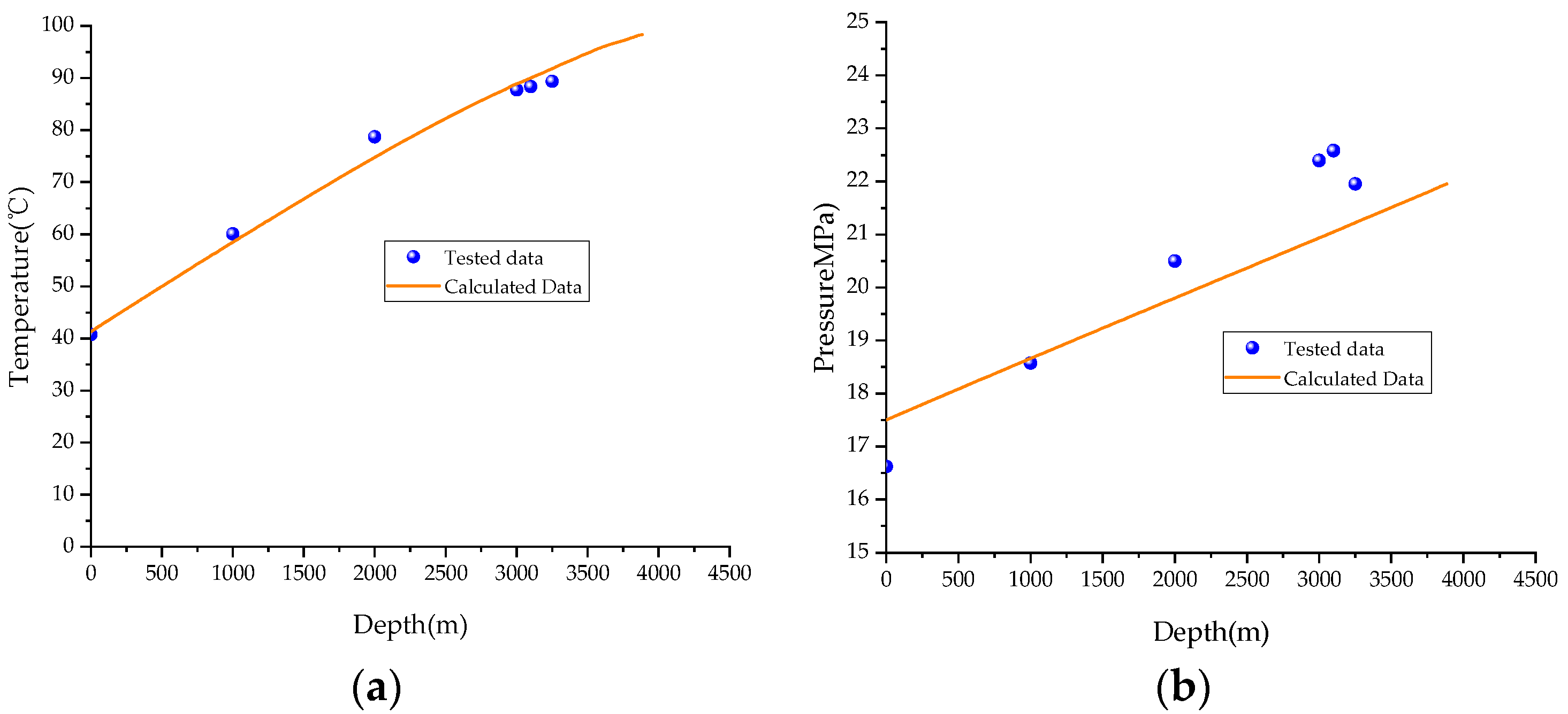
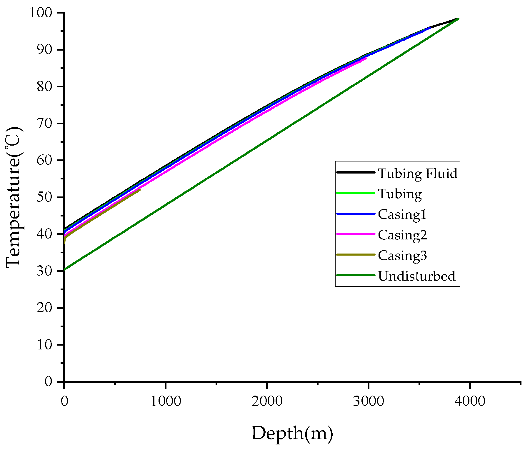
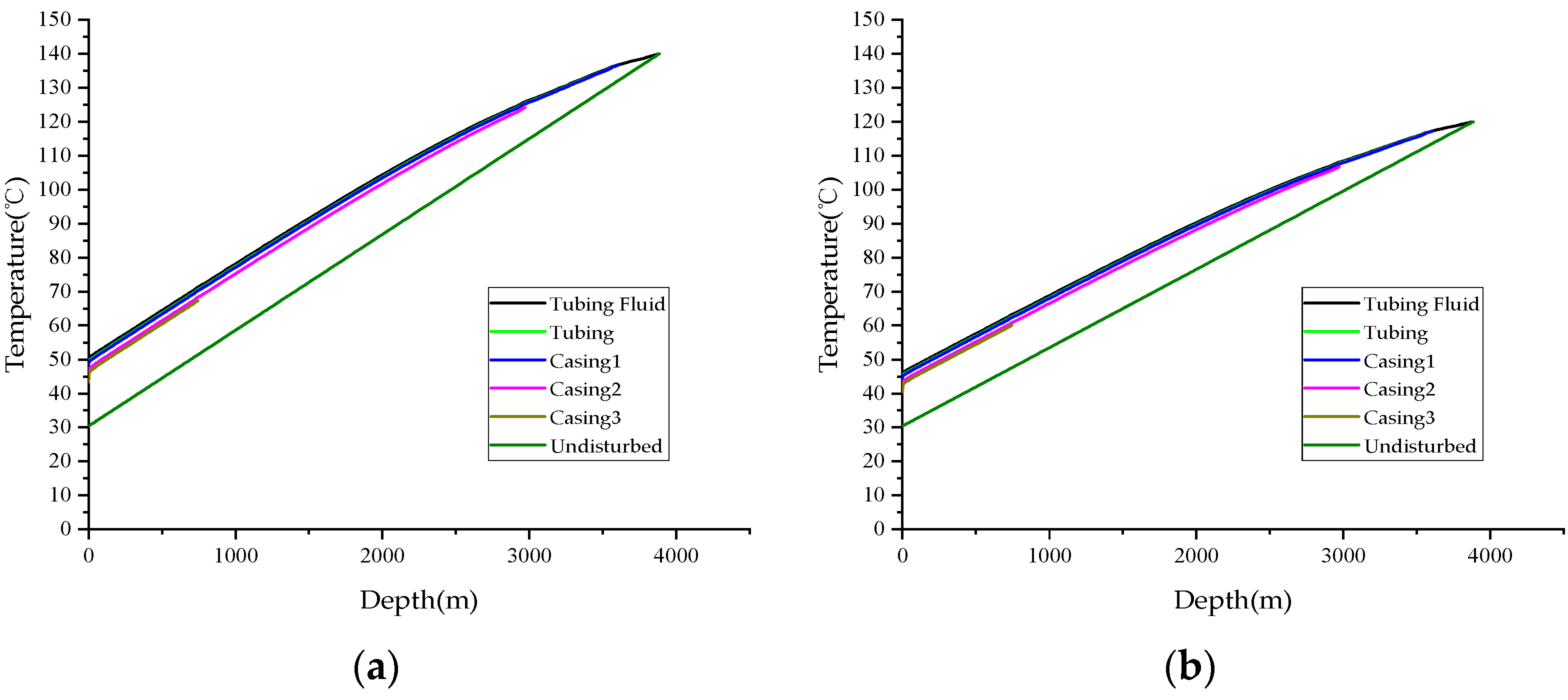
3. Validation
4. Discussion
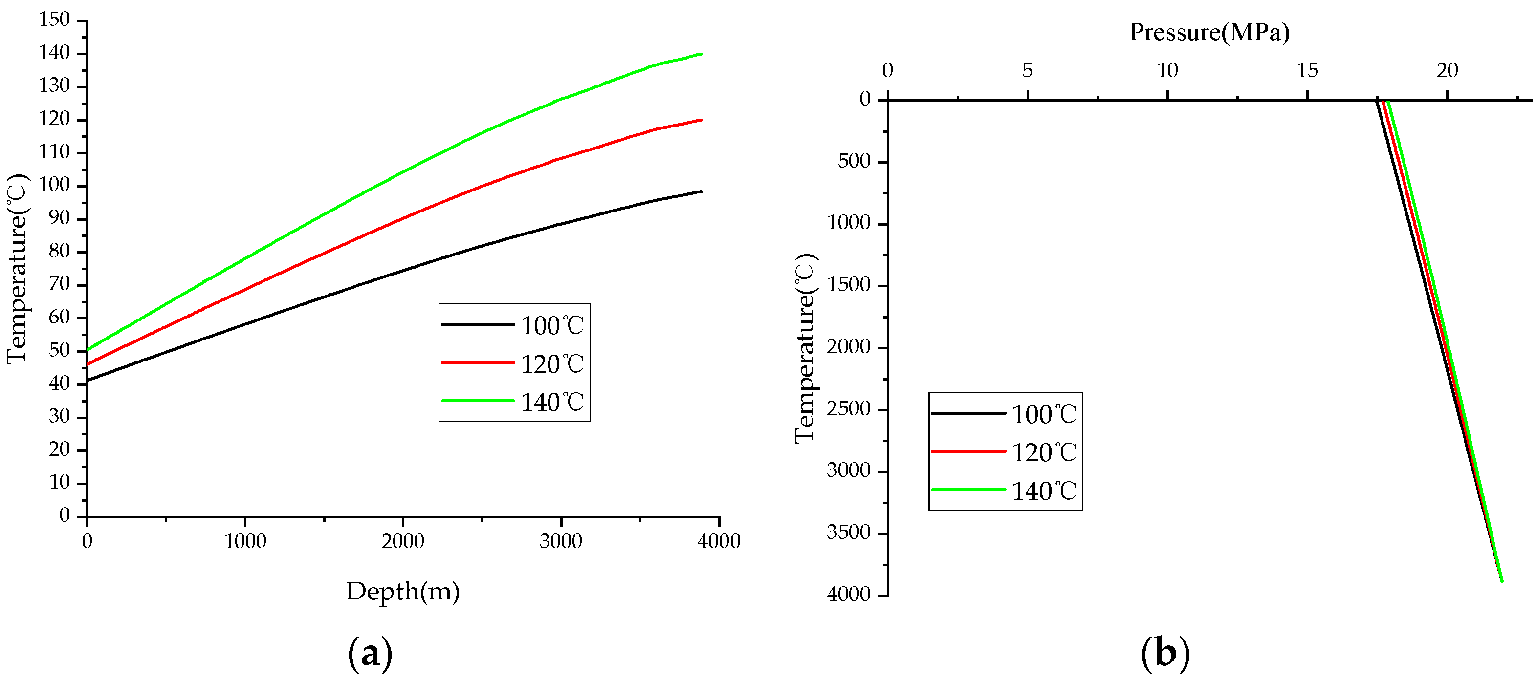
4.1. Gas Productivity
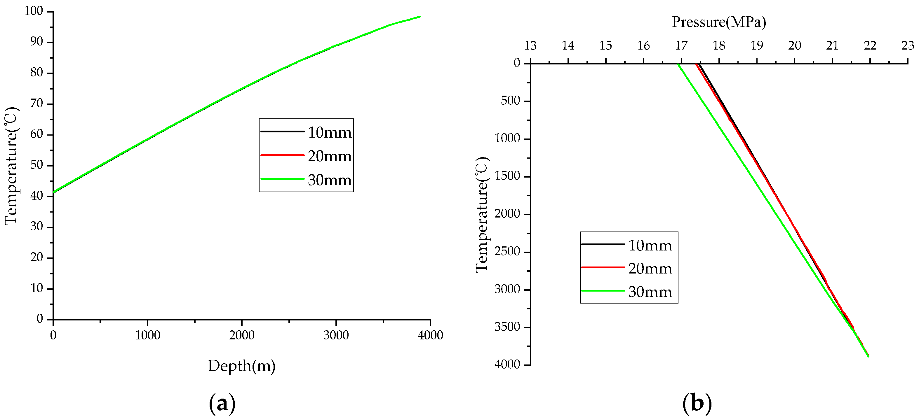
4.2. Sulfur Thickness
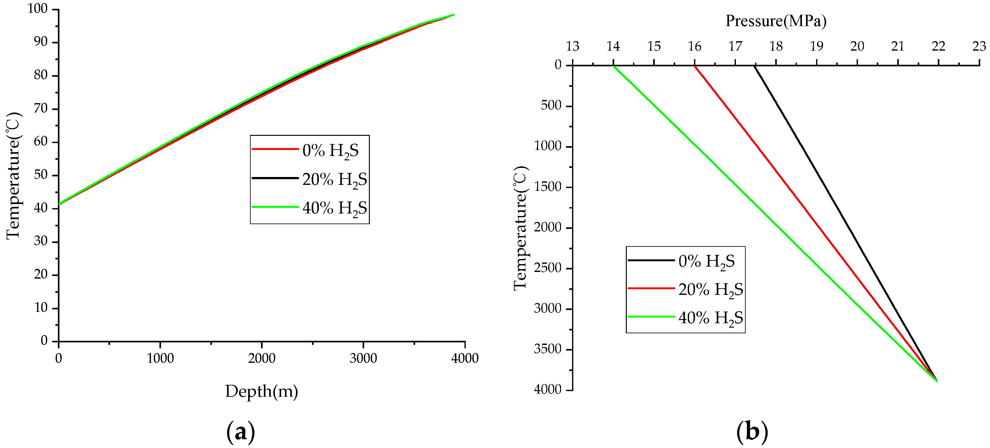
4.3. HSC
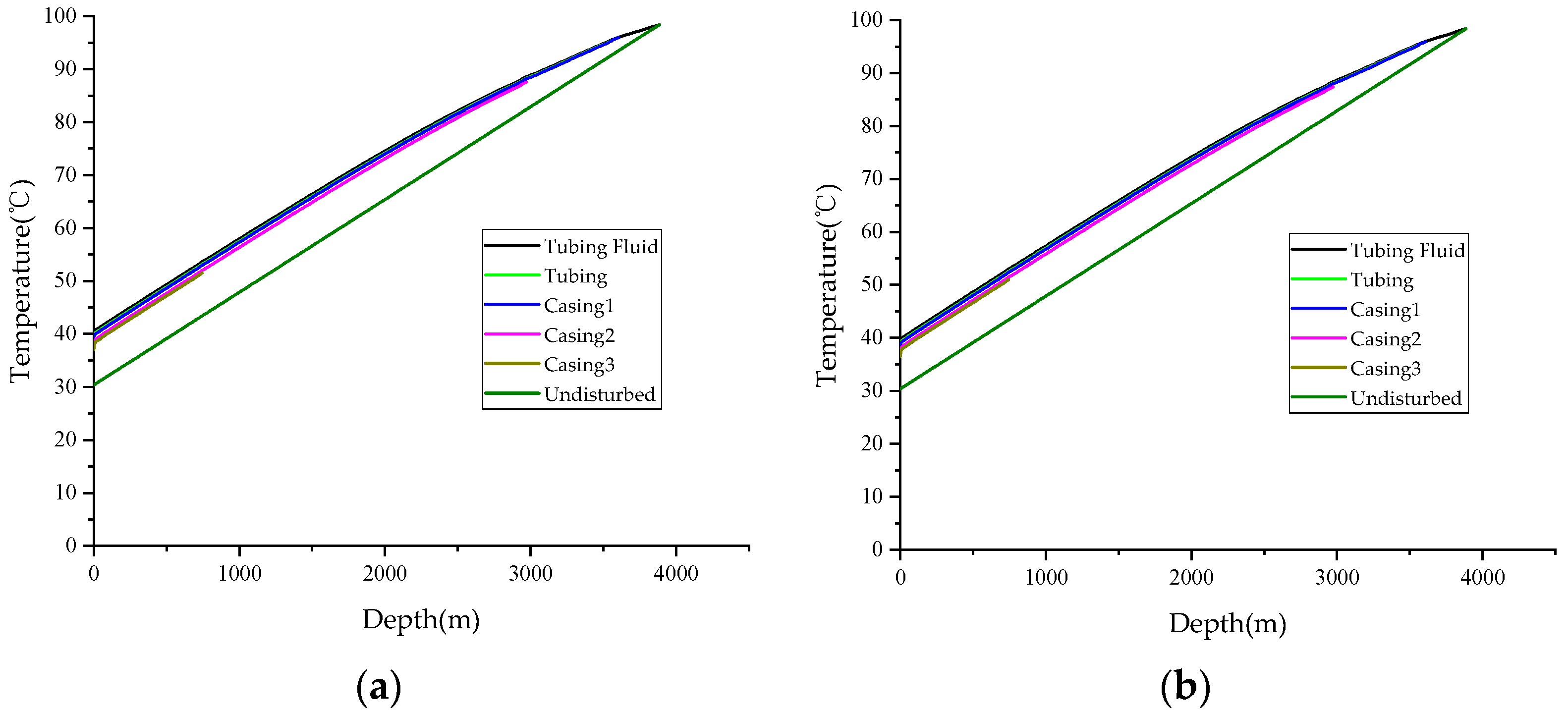
4.4. Reservoir Pressure
4.5. Reservoir Temperature
5. Conclusions
- (1)
- A temperature field prediction model incorporating sulfur deposition was developed, emphasizing variations in the PPPs of hydrogen-sulfide-containing gas and the corresponding modified model. The pressure model employed a GSTP flow approach, while the sulfur solubility prediction model selected a theoretical model tailored to the specific target block.
- (2)
- The accuracy of the calculation model is validated through comparison with field-measured data, revealing an error of 2.53% in the temperature calculations and 4.80% in the pressure calculations. The results demonstrate a high level of agreement, indicating that the model is suitable for predicting wellbore temperatures in HSG wells.
- (3)
- The production of the HSG well has a notable impact on temperature. Specifically, a 20.09% increase in the wellhead temperature is observed when comparing a gas production rate of 120 × 104 m3/d to that of 60 × 104 m3/d. The thickness of the sulfur scale within the wellbore influences the flow rate, subsequently leading to a decrease in wellhead pressure.
- (4)
- An elevation in the hydrogen sulfide concentration correlates with an increase in the density of natural gas, thereby causing a more rapid decline in pressure. This reduction in reservoir pressure and temperature will subsequently lower the wellbore pressure and temperature, impeding the removal of sulfur deposits at the well bottom and accelerating a decrease in the productivity of HSG wells.
- (5)
- This paper primarily examines a prediction model for temperature fields, without delving extensively into the specific locations and mechanisms of sulfur deposition under varying temperature conditions. Future research may explore these aspects further, enabling decision-makers to implement tailored strategies for sulfur deposition removal.
Author Contributions
Funding
Data Availability Statement
Conflicts of Interest
Abbreviations
| HSG | high-sulfur gas |
| GSTP | gas–solid two-phase |
| WTD | wellbore temperature distribution |
| PPP | physical property parameter |
| HSC | hydrogen sulfide content |
| Z | Deviation coefficient |
| Pseudo pressure | |
| Pseudo pressure | |
| Correction coefficient | |
| M | The sum of the mole fractions of H2S and CO2 in the system |
| N | The mole fraction of H2S in the system |
| Critical temperature, K | |
| Critical pressure, Pa | |
| Corrected critical temperature, K | |
| Corrected critical pressure, Pa | |
| Relative density of natural gas | |
| , | Viscosity correction values for H2S, CO2, and N2, respectively, mPa·s |
| H2S, CO2, N2 | Molar content in the gas mixture, % |
| Thermal conductivity coefficient, W/(m·K) | |
| T | Temperature, K |
| r | Distance from the center of the tubing, m |
| Heat capacity per unit volume, J/(m3·K) | |
| t | Time, s |
| Heat transfer coefficient, w/(m·K) | |
| Heat transfer coefficients of heat convection, w/(m·K) | |
| Heat transfer coefficients of heat radiation, w/(m·K) | |
| Content of sulfur particles | |
| Densities of sulfur particles, kg/m3 | |
| Densities of gas, kg/m3 | |
| Velocity of the solid sulfur particle, m/s | |
| Diameter of the sulfur particle, m | |
| Speed of the gas, m/s | |
| d | Inner diameter of the tubing, m |
| Viscosity of the gas, mPa·s | |
| Initial reservoir temperature at depth , K | |
| Wellhead temperature, K | |
| Temperature gradient, K/m | |
| Depth, m |
References
- Zhang, N.; Zhang, Z.; Rui, Z.; Li, J.; Zhang, C.; Zhang, Q.; Zhao, W.; Patil, S. Comprehensive risk assessment of high sulfur-containing gas well. J. Petrol. Sci. Eng. 2018, 170, 888–897. [Google Scholar] [CrossRef]
- Liu, W.; Huang, X.; Zhang, L.; He, J.; Cen, X. Analysis of sulfur deposition for high-sulfur gas reservoirs. Petrol. Sci. Technol. 2022, 40, 1716–1734. [Google Scholar] [CrossRef]
- Bemani, A.; Baghban, A.; Mohammadi, A.H. An insight into the modeling of sulfur content of sour gases in supercritical region. J. Petrol. Sci. Eng. 2020, 184, 106459. [Google Scholar] [CrossRef]
- Xu, Z.; Gu, S.; Zeng, D.; Sun, B.; Xue, L. Numerical simulation of sulfur deposit with particle release. Energies 2020, 13, 1522. [Google Scholar] [CrossRef]
- Piemjaiswang, R.; Khaisri, S.; Sema, T.; Chalermsinsuwan, B.; Nimmanterdwong, P. Performance of Data Segmentation ANN Model for Elemental Sulfur Solubility Prediction in Natural Gas Transportation Pipeline. In Proceedings of the 15th International Conference on Computer and Automation Engineering (ICCAE), Sydney, Australia, 3–5 March 2023. [Google Scholar]
- Sun, C.; Zeng, H.; Luo, J. Unraveling the effects of CO2 and H2S on the corrosion behavior of electroless Ni-P coating in CO2/H2S/Cl–environments at high temperature and high pressure. Corros. Sci. 2019, 148, 317–330. [Google Scholar] [CrossRef]
- Dong, B.; Liu, W.; Cheng, L.; Gong, J.; Wang, Y.; Gao, Y.; Dong, S.; Zhao, Y.; Fan, Y.; Zhang, T. Investigation on mechanical properties and corrosion behavior of rubber for packer in CO2-H2S gas well. Eng. Fail. Anal. 2021, 124, 105364. [Google Scholar] [CrossRef]
- Ramey, H.J., Jr. Wellbore heat transmission. J. Pet. Technol. 1962, 14, 427–435. [Google Scholar] [CrossRef]
- Willhite, G.P. Over-all heat transfer coefficients in steam and hot water injection wells. J. Pet. Technol. 1967, 19, 607–615. [Google Scholar] [CrossRef]
- Raymond, L.R. Temperature distribution in a circulating drilling fluid. J. Pet. Technol. 1969, 21, 333–341. [Google Scholar] [CrossRef]
- Eickmeier, J.R.; Ersoy, D.; Ramey, H.J. Wellbore temperatures and heat losses during production or injection operations. J. Can. Pet. Technol. 1970, 9, 115–121. [Google Scholar] [CrossRef]
- You, J.; Rahnema, H.; McMillan, M.D. Numerical modeling of unsteady-state wellbore heat transmission. J. Nat. Gas. Sci. Eng. 2016, 34, 1062–1076. [Google Scholar] [CrossRef]
- Dong, W.; Shen, R.; Liang, Q. Model calculations and factors affecting wellbore temperatures during SRV fracturing. Arab. J. Sci. Eng. 2018, 43, 6475–6480. [Google Scholar] [CrossRef]
- Hasan, A.R.; Kabir, C.S. Aspects of wellbore heat transfer during two-phase flow. Spe Prod. Facil. 1994, 9, 211–216. [Google Scholar] [CrossRef]
- Kabir, C.S.; Hasan, A.R.; Jordan, D.L.; Wang, X. A wellbore/reservoir simulator for testing gas wells in high-temperature reservoirs. Spe Form. Eval. 1996, 11, 128–134. [Google Scholar] [CrossRef]
- Hasan, A.R.; Kabir, C.S.; Wang, X. Wellbore two-phase flow and heat transfer during transient testing. Spe J. 1998, 3, 174–180. [Google Scholar] [CrossRef]
- Wang, Y.; Ye, J.; Wu, S. A prediction model of wellbore temperature and pressure distribution in hydrocarbon gas injection well, In Proceedings of 5th International Workshop on Renewable Energy and Development, Chengdu, China, 23–25 April 2021.
- Sun, W.; Wei, N.; Zhao, J.; Zhou, S.; Zhang, L.; Li, Q.; Jiang, L.; Zhang, Y.; Li, H.; Xu, H. Wellbore temperature and pressure field in deep-water drilling and the applications in prediction of hydrate formation region. Front. Energy Res. 2021, 9, 696392. [Google Scholar] [CrossRef]
- Zheng, J.; Dou, Y.; Li, Z.; Yan, X.; Zhang, Y.; Bi, C. Investigation and application of wellbore temperature and pressure field coupling with gas–liquid two-phase flowing. J. Pet. Explor. Prod. Technol. 2022, 12, 753–762. [Google Scholar] [CrossRef]
- An, J.; Li, J.; Huang, H.; Liu, G.; Chen, S.; Zhang, G. Numerical study of temperature–pressure coupling model for the horizontal well with a slim hole. Energy Sci. Eng. 2023, 11, 1060–1079. [Google Scholar] [CrossRef]
- Chen, X.; Wang, S.; He, M.; Xu, M. A comprehensive prediction model of drilling wellbore temperature variation mechanism under deepwater high temperature and high pressure. Ocean. Eng. 2024, 296, 117063. [Google Scholar] [CrossRef]
- Brunner, E.; Place, M.C., Jr.; Woll, W.H. Sulfur solubility in sour gas. J. Pet. Technol. 1988, 40, 1587–1592. [Google Scholar] [CrossRef]
- Serin, J.; Jay, S.; Cézac, P.; Contamine, F.; Mercadier, J.; Arrabie, C.; Legros-Adrian, J. Experimental studies of solubility of elemental sulphur in supercritical carbon dioxide. J. Supercrit. Fluids 2010, 53, 12–16. [Google Scholar] [CrossRef]
- Cloarec, E.; Serin, J.; Cézac, P.; Contamine, F.; Mercadier, J.; Louvat, A.; Casola Lopez, A.; Van Caneghem, P.; Forster, R.; Kim, U. Experimental studies of solubility of elemental sulfur in methane at 363.15 K for pressure ranging from (4 to 25) MPa. J. Chem. Eng. Data 2012, 57, 1222–1225. [Google Scholar] [CrossRef]
- Yang, X.F.; Huang, X.P.; Zhong, B. Experimental test and calculation methods of elemental sulfur solubility in high sulfur content gas. Nat. Gas. Geosci. 2009, 20, 416. [Google Scholar]
- Guo, X.; Wang, Q. A new prediction model of elemental sulfur solubility in sour gas mixtures. J. Nat. Gas. Sci. Eng. 2016, 31, 98–107. [Google Scholar] [CrossRef]
- Wang, Q.; Guo, X.; Leng, R. In-depth study on the solubility of elemental sulfur in sour gas mixtures based on the Chrastil’s association model. Petroleum 2016, 2, 425–434. [Google Scholar] [CrossRef]
- Karan, K.; Heidemann, R.A.; Behie, L.A. Sulfur solubility in sour gas: Predictions with an equation of state model. Ind. Eng. Chem. Res. 1998, 37, 1679–1684. [Google Scholar] [CrossRef]
- Wei, Y.; Wang, L.; Yang, Y.; Wen, L.; Huo, X.; Zhang, L.; Yang, M. Molecular mechanism in the solubility reduction of elemental sulfur in H2S/CH4 mixtures: A molecular modeling study. Fluid. Phase Equilibr 2023, 569, 113764. [Google Scholar] [CrossRef]
- Heidemann, R.A.; Phoenix, A.V.; Karan, K.; Behie, L.A. A chemical equilibrium equation of state model for elemental sulfur and sulfur-containing fluids. Ind. Eng. Chem. Res. 2001, 40, 2160–2167. [Google Scholar] [CrossRef]
- Kadoura, A.; Salama, A.; Sun, S.; Sherik, A. An NPT monte carlo molecular simulation-based approach to investigate solid-vapor equilibrium: Application to elemental sulfur-H2S system. Procedia Comput. Sci. 2013, 18, 2109–2116. [Google Scholar] [CrossRef]
- ZareNezhad, B.; Aminian, A. Predicting the sulfur precipitation phenomena during the production of sour natural gas by using an artificial neural network. Petrol. Sci. Technol. 2011, 29, 401–410. [Google Scholar] [CrossRef]
- Mehrpooya, M.; Mohammadi, A.H.; Richon, D. Extension of an artificial neural network algorithm for estimating sulfur content of sour gases at elevated temperatures and pressures. Ind. Eng. Chem. Res. 2010, 49, 439–442. [Google Scholar] [CrossRef]
- Dranchuk, P.M.; Purvis, R.A.; Robinson, D.B. Computer calculation of natural gas compressibility factors using the Standing and Katz correlation. In Proceedings of the Annual Technical Meeting, Edmonton, AB, Canada, 7–11 May 1973. [Google Scholar]
- Wichert, E.; Aziz, K. Calculate Zs for sour gases. Hydrocarb. Process. 1972, 51, 119. [Google Scholar]
- Dempsey, J.R. Computer routine treats gas viscosity as a variable. Oil Gas J. 1965, 63, 141–143. [Google Scholar]
- Standing, M.B. Volumetric and phase behavior of oil field hydrocarbon systems. In Society of Petroleum Engineers of AIME; Society of Petroleum Engineers of AIME: Wilkes-Barre, PA, USA, 1952. [Google Scholar]
- Shuai, X.; Meisen, A. New correlations predict physical properties of elemental sulfur. Oil Gas J. 1995, 93, 116529. [Google Scholar]
- Colebrook, C.F.; Blench, T.; Chatley, H.; Essex, E.H.; Finniecome, J.R.; Lacey, G.; Williamson, J.; Macdonald, G.G. Correspondence. turbulent flow in pipes, with particular reference to the transition region between the smooth and rough pipe laws. J. Inst. Civ. Eng. 1939, 12, 393–422. [Google Scholar] [CrossRef]
- Chrastil, J. Solubility of solids and liquids in supercritical gases. J. Phys. Chem. 1982, 86, 3016–3021. [Google Scholar] [CrossRef]
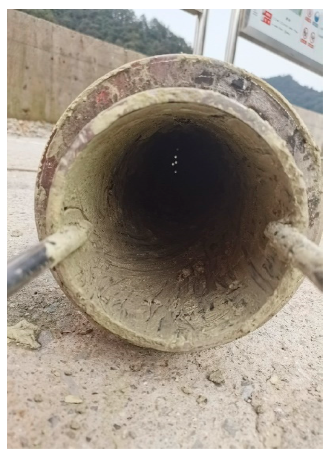
- FU, D. Dynamic Characteristics and Countermeasures of Sulfur Plugging in Gas Wells of Puguang Gas Field. J. Southwest Pet. Univ. 2023, 45, 119–130. [Google Scholar]
- Guo, X.; Wang, P.; Ma, J.; Jia, C. Numerical Simulation of Sulfur Deposition in Wellbore of Sour-Gas Reservoir. Processes 2022, 10, 1743. [Google Scholar] [CrossRef]


| A1 | 0.31506237 | A5 | −0.61232032 |
| A2 | −1.0467099 | A6 | −0.10488813 |
| A3 | −0.57832729 | A7 | 0.68157001 |
| A4 | 0.53530771 | A8 | 0.68446549 |
| B0 | −2.4621182 | B6 | 0.36037302 | B12 | 0.0839387178 |
| B1 | 2.97054714 | B7 | −0.0104432413 | B13 | −0.186408846 |
| B2 | −0.286264054 | B8 | −0.793385684 | B14 | 0.0203367881 |
| B3 | 0.00805420522 | B9 | 1.39643306 | B15 | −0.000609579263 |
| B4 | 2.80860949 | B10 | −0.149144925 | ||
| B5 | −3.49803305 | B11 | 0.00441015512 |
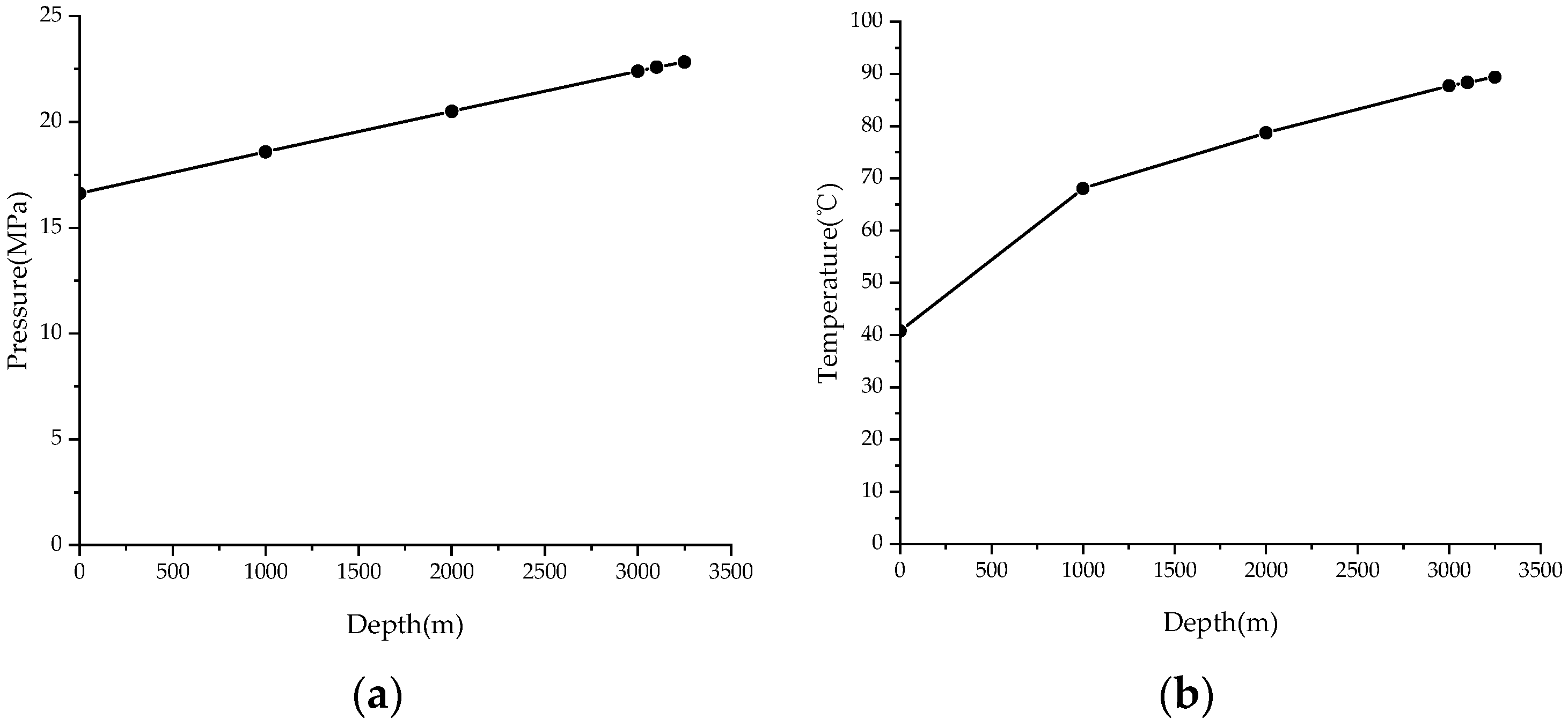
| Depth (m) | True Vertical Depth (m) | Pressure (MPa) | Pressure Gradient (MPa/100 m) | Temperature (°C) | Temperature Gradient (°C/100 m) |
|---|---|---|---|---|---|
| 0.00 | 0.00 | 16.620 | / | 40.78 | / |
| 1000.00 | 999.99 | 18.584 | 0.196 | 68.06 | 2.73 |
| 2000.00 | 1999.26 | 20.497 | 0.191 | 78.72 | 1.07 |
| 3000.00 | 2998.94 | 22.394 | 0.190 | 87.73 | 0.90 |
| 3100.00 | 3097.32 | 22.580 | 0.189 | 88.37 | 0.65 |
| 3250.00 | 3229.07 | 21.953 | 0.257 | 89.37 | 0.76 |
| Component | Na2O | MgO | Al2O3 | SiO2 | P2O5 | SO3 | Cl | K2O |
| Mass ratio | 0.0905 | 0.1089 | 0.8055 | 1.6912 | 0.0174 | 3.6514 | 0.0305 | 0.0828 |
| Component | CaO | Fe2O3 | NiO | CuO | ZnO | SrO | BaO | S |
| Mass ratio | 0.1676 | 0.4706 | 0.0087 | 0.0154 | 0.1239 | 0.0202 | 8.0479 | 84.668 |
Disclaimer/Publisher’s Note: The statements, opinions and data contained in all publications are solely those of the individual author(s) and contributor(s) and not of MDPI and/or the editor(s). MDPI and/or the editor(s) disclaim responsibility for any injury to people or property resulting from any ideas, methods, instructions or products referred to in the content. |
© 2024 by the authors. Licensee MDPI, Basel, Switzerland. This article is an open access article distributed under the terms and conditions of the Creative Commons Attribution (CC BY) license (https://creativecommons.org/licenses/by/4.0/).
Share and Cite
Fang, Q.; He, J.; Wang, Y.; Pan, H.; Ren, H.; Liu, H. A Predictive Model for Wellbore Temperature in High-Sulfur Gas Wells Incorporating Sulfur Deposition. Processes 2024, 12, 1073. https://doi.org/10.3390/pr12061073
Fang Q, He J, Wang Y, Pan H, Ren H, Liu H. A Predictive Model for Wellbore Temperature in High-Sulfur Gas Wells Incorporating Sulfur Deposition. Processes. 2024; 12(6):1073. https://doi.org/10.3390/pr12061073
Chicago/Turabian StyleFang, Qiang, Jinghong He, Yang Wang, Hong Pan, Hongming Ren, and Hao Liu. 2024. "A Predictive Model for Wellbore Temperature in High-Sulfur Gas Wells Incorporating Sulfur Deposition" Processes 12, no. 6: 1073. https://doi.org/10.3390/pr12061073
APA StyleFang, Q., He, J., Wang, Y., Pan, H., Ren, H., & Liu, H. (2024). A Predictive Model for Wellbore Temperature in High-Sulfur Gas Wells Incorporating Sulfur Deposition. Processes, 12(6), 1073. https://doi.org/10.3390/pr12061073