Study of Methane Solubility Calculation Based on Modified Henry’s Law and BP Neural Network

Abstract

Methane (CH₄), a non-polar molecule characterized by a tetrahedral structure, stands as the simplest organic compound. Predominantly constituting conventional natural gas, shale gas, and combustible ice, it plays a pivotal role as a carbon-based resource and a key raw material in the petrochemical industry. In natural formations, CH₄ and H₂O coexist in a synergistic system. This interplay necessitates a thorough examination of the phase equilibrium in the CH₄-H₂O system and CH₄’s solubility under extreme conditions of temperature and pressure, which is crucial for understanding the genesis and development of gas reservoirs. This study synthesizes a comprehensive solubility database by aggregating extensive solubility data of CH₄ in both pure and saline water. Utilizing this database, the study updates and refines the key parameters of Henry’s law. The updated Henry’s law has a prediction error of 22.86% at less than 40 MPa, which is an improvement in prediction accuracy compared to before the update. However, the modified Henry’s law suffers from poor calculation accuracy under certain pressure conditions. To further improve the accuracy of solubility prediction, this work also trains a BP (Back Propagation) neural network model based on the database. In addition, MSE (Mean-Square Error) is used as the model evaluation index, and pressure, temperature, compression coefficient, salinity, and fugacity are preferred as input variables, which finally reduces the mean relative error of the model to 16.32%, and the calculation results are more accurate than the modified Henry’s law. In conclusion, this study provides a novel and more accurate method for predicting CH₄ solubility by comparing modified Henry’s law to neural network modeling.

1. Introduction

CH₄ is ubiquitously found in nature, being the simplest organic compound and the hydrocarbon with the lowest carbon content. Its formation and distribution vary greatly, ranging from deep geological strata to shallow coalbeds, CH₄ hydrates, biogas, industrial outputs, and even in extraterrestrial environments. The solubility of CH₄ profoundly influences the genesis and evolution of natural gas reservoirs, bearing crucial implications for the methodologies deployed in evaluating and harnessing these reserves. Influenced by a multitude of variables including temperature, pressure, the chemical composition of water, and the presence of other gases, CH₄’s solubility exhibits notable variations. Notably, a decrease in temperature or an increase in pressure augments CH₄’s solubility, a phenomenon critically pivotal for the genesis of CH₄ hydrates. Moreover, the presence of salts and other solutes can subtly modulate CH₄’s solubility through alterations in water’s chemical activity. Consequently, an in-depth comprehension of CH₄’s dissolution characteristics under varied conditions is indispensable for the effective prediction and management of natural gas resources. Given CH₄’s role as a significant greenhouse gas, its solubility dynamics within aquatic environments also play an indispensable role in global climate change research. Hence, investigating CH₄ solubility across diverse environmental scenarios not only enriches our understanding of natural gas reservoir formation and distribution but also holds paramount scientific relevance to environmental and climate sciences [1].

In 1931, Frolich pioneered the study of CH₄ solubility under specific pressure conditions (2 to 14.2 MPa), establishing that, barring compound formation with the solvent, gas behavior largely adheres to Henry’s Law within an acceptable engineering error margin [2]. In 1979, Price [3] expanded this research to a broader temperature and pressure scope (150 °C to 350 °C, 7 to 200 MPa), noting significant solubility increases with temperature. However, the applicability of these results under extreme conditions, particularly above 250 °C, was limited due to notable deviations. Ou [4] et al. employed quantitative Raman spectroscopy to methodically assess CH₄ solubility in pure water across 0 to 330 °C and 5 to 140 MPa. Their findings from 43 to 263 °C align with prior experimental and thermodynamic research, leading to precise CH₄ solubility calculations within this temperature range. Notwithstanding, their method, involving a small, non-sampling approach, overlooked water vapor’s impact, a significant factor under high-temperature, high-pressure conditions. At temperatures below 20 °C, CH₄ solubility testing diverges from established natural gas hydrate data due to potential hydrate formation.

In exploring CH₄ solubility in pure water, Duffy [5], Krader [6], Fan [7], and others investigated salt ions’ impact in simulated formation water. Their results indicate that CH₄ solubility in formation water, while following similar patterns to pure water, is marginally lower under identical temperature and pressure conditions. With increasingly comprehensive and uniformly distributed temperature–pressure solubility data, many researchers have devised solubility models for CH₄ in pure and formation water, employing state equation and activity coefficient methods, continually refined with new data. These models predominantly cover 0 to 250 °C and 0.1 to 200 MPa, with brine salinity ranging up to 6 mol/kg. Duan [8] introduced a semi-empirical predictive model based on state equations and particle interaction theory, subsequently optimized for better accuracy and range in predicting gases like CH₄, H₂S, and CO₂ solubility.

Recently, Artificial Neural Networks (ANNs) have emerged as a prominent research area in artificial intelligence, offering practical solutions across various fields, including mathematics, pharmacology, economics, psychology, and neurology [9]. The study by Li et al. [10] develops a method to predict gas solubility in polymers using a neural network optimized by chaos theory and a self-adaptive particle swarm optimization, improving accuracy significantly over traditional methods. In the study by Mohammadi et al. [11], adaptive boosting support vector regression (AdaBoost-SVR) models were developed and demonstrated superior accuracy over traditional equations of state in predicting the solubility of light hydrocarbon gases in brine under diverse conditions. Taherdangkoo et al. [12] demonstrated the application of machine learning algorithms, including boosted regression trees optimized with Bayesian optimization, to accurately predict CH₄ solubility in water and seawater across a range of temperatures and pressures, achieving a high coefficient of determination (R² = 0.99). Deng and Guo [13] developed an artificial neural network model to predict the products of CH₄ bi-reforming using CO₂ and steam, demonstrating its accuracy with correlation coefficients over 0.995 across various operational conditions. Li et al. [14] developed two neural network models to predict CO₂ solubility in aqueous blended amine solvents, using extensive experimental data and a backpropagation learning algorithm. The models demonstrated high accuracy, outperforming traditional thermodynamic models, and were particularly effective for complex blended amine systems like MDEA/PZ and MEA/MDEA/PZ. M.E. Hamzehie et al. [15] developed a feed-forward multilayer neural network to predict the solubility of CO₂ in mixed aqueous solutions of amines, covering a wide range of temperatures, pressures, and concentrations. The model, using the Levenberg–Marquardt back-propagation algorithm combined with Bayesian regularization, demonstrated high accuracy, significantly outperforming traditional thermodynamic models. Mokarizadeh et al. [16] demonstrated that a Least Square Support Vector Machine (LSSVM) model, enhanced with a genetic algorithm, provides a highly accurate prediction of SO₂ solubility in various ionic liquids, outperforming conventional Artificial Neural Network models. The research by Mohammadi et al. [17] advances the field of SO₂ solubility prediction in ionic liquids by employing four soft computing approaches and five equations of state. They find the Deep Belief Network model to offer the most reliable solubility predictions, significantly outperforming traditional equations of state. The above study illustrates the suitability of ANN for analyzing and predicting the solubility of gases due to its learning ability, speed, and accuracy; hence, this method is used in this study to predict the solubility of CH₄.

In this paper, an extensive survey and compilation of solubility data for CH₄ in pure and saline water has resulted in a comprehensive database. Using this comprehensive database, this work first updates and corrects the relevant parameters of Henry’s law and uses the corrected Henry’s law for CH₄ solubility prediction. However, the modified Henry’s law is still not applicable under certain conditions [18]. Therefore, a BP neural network model has also been developed in this work to provide more accurate predictions of CH₄ solubility in water.

2. CH₄ Solubility Data Collection and Processing

2.1. CH₄ Solubility Data Collection

In a comprehensive review spanning the literature from 1936 to 2022, this work meticulously curated approximately 1300 data detailing the solubility of CH₄ across a diverse spectrum of conditions, encompassing variations in pressure, temperature, and mineral content. The specific ranges of these parameters, along with corresponding solubility values, are systematically presented in

Table 1. CH₄ Solubility Data.

References	Pressure MPa	Temperature K	Salinity g/L	Solubility mol/mol
[4]	5~140	273.15~603.15	0	0.00065~0.073
[2]	0.567~9.08	274~285.68	0	0.00026~0.002
[19]	1.151~10.36	283.14~298.15	0	0.00038~0.0021
[20]	1~2.7	274.15~284.65	0	0.00033~0.0015
[21]	2~40.03	283.2~303.2	0	0.00056~0.0041
[22]	0.34~9.26	313.35~373.29	0	0.00005~0.0015
[23]	0.567~9.08	274.2~285.6	0	0.00025~0.0022
[24]	4.06~46.91	298.15~423.15	0~315.9	0.00017~0.003
[5]	0.317~6.52	298.15~303.15	0~315.9	0.00007~0.00113
[3]	0.101325~200	273.15~633.20	0	0.000016~0.18
[25]	10.1325~61.61	298.15~398.15	0~234	0.00081~0.0043
[26]	4.137~34.47	310.93~344.26	0	0.000602~0.00335
[27]	1.327~6.451	297.50~518.30	0	0.00021~0.00103

.

Figure 1 illustrates the relationship between the solubility of CH₄ gas in water and its environmental conditions. Specifically, at a constant temperature, CH₄’s solubility in water escalates with an increase in pressure. Conversely, at a constant pressure with temperatures below 373.15 K, its solubility diminishes as temperature rises. However, in environments where the pressure remains constant but the temperature exceeds 433.15 K, we observe CH₄’s solubility augmenting in response to higher temperatures. Figure 2 depicts the solubility of CH₄ in a 3.519 g/L NaCl solution under the same range of temperatures (from 298.15 K to 423.15 K) but at a narrower pressure range of 4 to 24 MPa. Similar to Figure 1, CH₄’s solubility increases with pressure. However, the overall solubility in the saline solution is lower than in pure water for equivalent temperatures and pressures. Additionally, the influence of temperature on solubility in the saline solution is less pronounced, and the solubility lines are closer together, indicating a reduced temperature dependency compared to pure water. When comparing both figures, it is clear that the presence of NaCl in the solution reduces the solubility of CH₄ and modifies the solubility behavior with respect to temperature.

2.2. Data Processing

Upon collecting an extensive dataset, the foremost task is data processing. High-quality data processing is paramount for the efficacy of model training. It enhances not only the efficiency and performance of the model but also significantly bolsters the model’s adaptability to new data and its generalization capabilities, which are crucial for augmenting the accuracy of CH₄ solubility predictions. In this study, we processed the collected CH₄ solubility data as follows:

1.

Outlier Removal [28]

The presence of outliers can skew the outcomes of model training. Therefore, outlier identification and removal are critical in the data preprocessing phase. We used the interquartile spacing (IQR) method to identify and reject outliers in the collected CH₄ solubility data. We grouped the collected solubility data by similar pressure and temperature conditions and used the IQR method for each group. According to this method, outliers are defined by the criterion that any data point less than x is considered a low-end outlier and any data point greater than y is considered a high-end outlier. Where Q₁ (first quartile) represents 25% of all data points less than or equal to this value, Q₃ (third quartile) represents 75% of all data points less than or equal to this value, and IQR represents the difference between Q₃ and Q₁.

Where the values of x and y are:

$$x=Q_1-1.5\times IQR$$

(1)

$$y=Q_3+1.5\times IQR$$

(2)

Given the minimal number of outliers detected, we opted to remove these data points, a decision grounded in maintaining data integrity and ensuring analytical precision.

2.

Data Standardization [29]

Addressing the diversity of units used to express solubility across different sources necessitated the standardization of our dataset to a uniform unit for analysis and computation. We standardized all solubility measurements to mol/mol, thereby streamlining the data processing workflow and guaranteeing uniformity in our analytical approach.

3.

Processing Data Under Identical Conditions

For post-outlier removal and data standardization, we aggregated the solubility measurements obtained under identical experimental conditions by calculating their mean. This method aimed to mitigate the impact of individual measurement discrepancies and enhance the overall stability and reliability of our findings.

After data collection and processing, we chose a pressure range of 1.482 MPa to 120 MPa, with a total of 1069 data points.

3. Prediction of CH₄ Solubility Based on Revised Henry’s Law

3.1. Henry’s Law

If the solubility of gas in water is very small, the solubility of gas in water is proportional to its fugacity:

$$f_g^v=H{x}_g$$

(3)

where $f_g^v$ is gas fugacity, $H$ is Henry’s coefficient, and $x_g$ is solubility of gas components in water.

Under low-pressure conditions, Henry’s coefficient H can be approximated as a function of temperature, and the influence of pressure can be ignored. However, Henry’s law is not applicable to other pressure ranges. For high-pressure systems, the influence of pressure on Henry’s law cannot be ignored. Vul’fson and Borodin [30] proposed an extension of Henry’s law based on the Van’t Hoff model of concentrated solutions, with an important modification to Henry’s law, in order to describe more accurately the behavior of real gases under varying conditions of temperature and pressure. Therefore, in this paper, Henry’s coefficient H is modified when the law is used to predict the solubility of CH₄.

3.2. Effect of Hydrate Formation on Solubility

In the process of hydrate formation, the solubility of CH₄ gas in water has a large deviation from the solubility calculated by the traditional model, which is because the process of hydrate formation is different from the process of gas dissolution in water, and the water molecules will surround the CH₄ gas molecules to form a cage-like structure when generating the gas hydrate, which greatly increases the solubility of the gas molecules in the water, which makes it difficult to study the solubility law of CH₄ gas in water.

Peter Englezos [31] in 1988 calculated the stability limit of aqueous solutions of CH₄ using the Trebble–Bishnoi equation of state for a range of temperatures and pressures chosen to be in the region of hydrate formation, and found that the solubility of the gas increases with temperature when the pressure is constant, but that the mole fraction of the solubility of CH₄ under hydrate-generating conditions is much higher than the molar fraction in the gas–liquid phase, which may be due to the hydrate nucleation process.

Song et al. [32] in 1997 measured the solubility of CH₄ and ethane gases in water under different conditions, the experimental conditions included temperature and pressure conditions for hydrate formation, where CH₄ gas was measured at a pressure of 3.45 MPa and temperatures between 273.2 K and 290.2 K. They found that the solubility data were significantly different with decreasing temperature. The solubility data obtained with decreasing temperature differed significantly from the solubility calculated by Henry’s law.

Therefore, in the presence of hydrate formation, relying solely on the actual temperature and pressure is inadequate for determining the solubility of gas in water. When the temperature is fixed, if the hydrate formation pressure exceeds the actual pressure, it indicates the absence of hydrate formation. In such cases, the actual pressure should be utilized; conversely, when the hydrate formation pressure is lower, the pressure of hydrate formation should be employed. Similarly, when the pressure remains constant, if the hydrate formation temperature surpasses the actual temperature, hydrate formation occurs, necessitating the utilization of the hydrate formation temperature; otherwise, the actual temperature is applied. This study adopts an approach where the pressure utilized in calculating the solubility of CH₄ in water is adjusted when the temperature satisfies the conditions for hydrate formation. The CH₄ hydrate formation curve is shown in Figure 3.

3.3. Modification of Henry’s Coefficient of CH₄

According to the SRK equation of state:

$$P=\frac{RT}{V-b}-\frac{a\left(T\right)}{V(V+b)}$$

(4)

According to the known temperature and pressure, the compression factor can be obtained, and the fugacity can be derived from the compression factor. Then, according to Henry’s law, Henry’s coefficient H can be obtained. The obtained Henry’s coefficient H is fitted with temperature T, pressure P, and salinity W to obtain a new functional relationship:

$$H=f(T,P,W)$$

(5)

Because of the large pressure range, one-part equations do not apply well to the entire pressure range and need to be fitted with two-part equations. After a number of pressure range divisions, it was found that the solubility data in both ranges fitted better with 40 MPa as the cutoff point.

• P ≤ 40 MPa

The fitting equation for the modified Henry coefficient H is:

$$H=\mathrm{A}\mathrm{B}\mathrm{S}(a+b_1{x}_1+b_2{x}_1^2+b_3{x}_2+b_4{x}_2^2+b_5{x}_3+b_6{x}_1{x}_3+b_7{x}_1^2{x}_3)$$

(6)

where H is the Henry coefficient; x₁ is the pressure, MPa; x₂ is the temperature, K; x₃ is the salinity, g/L; and a, b₁, b₂, b₃, b₄, b₅, b₆, b₇ are the fitting coefficients, with specific values shown in

Table 2. Coefficients for pressures less than or equal to 40 MPa.

Coefficients	Values
a	−30,352,612,628.3169
b1	117,170,471.025335
b2	−1,833,088.19361018
b3	175,581,561.321355
b4	−209,307.407123789
b5	24,472,236.0289736
b6	4,156,153.62314121

.

The average relative error is 22.86%, and the comparison of predicted and actual values, as well as the average relative error, is shown in Figure 4.

2.

P > 40 MPa

The fitting equation for the modified Henry coefficient H is:

$$\begin{gathered} H=\mathrm{A}\mathrm{B}\mathrm{S}(a+b_1{x}_2^2+b_2{x}_2{x}_3+b_3{x}_3{x}_1^2+b_4{x}_3{x}_1+b_5{x}_2{x}_3{x}_1+b_6{x}_2^2+b_7{x}_2 \\ +b_8{x}_1^2+b_9{x}_1+b_{10}{x}_2{x}_1) \end{gathered}$$

(7)

where H is the Henry coefficient; x₁ is the pressure, MPa; x₂ is the temperature, K; x₃ is the salinity, g/L; and a, b₁, b₂, b₃, b₄, b₅, b₆, b₇, b₈, b₉, b₁₀ are the fitting coefficients, with specific values shown in

Table 3. Coefficients for pressures greater than 40 MPa.

Coefficients	Values
a	−5,311,667,915.66811
b1	1603.92554912757
b2	−1,033,012.08072614
b3	−102,060.909835676
b4	9,677,746.84501353
b5	1727.13635637011
b6	−157,130.38162931
b7	109,837,329.146691
b8	396,002.273542842
b9	−185,624,382.240331
b10	169,960.110823592

.

The average relative error is 32.67%, and the comparison of predicted and actual values, as well as the average relative error, is shown in Figure 5.

3.4. Prediction of CH₄ Gas Solubility

Figure 4 and Figure 5 illustrate the solubility data of CH₄ gas in water under two distinct pressure conditions, derived from Henry’s Law with correction coefficients. These data show a strong correlation with experimental results. Specifically, at pressures below 40 MPa, the average relative error in the CH₄ solubility data calculated using the modified Henry’s Law is 22.86%, enhancing the accuracy of the predictions. At pressures lower than 10 MPa, the average deviation of the solubility of CH₄ gas in water calculated by Henry’s coefficient H using the empirical formula [33] of the previous authors is 48.6%, so this paper has a much smaller error than that of the empirical formula and has a better prediction performance. However, above 40 MPa, the average relative error increases to 32.67%, indicating a significant discrepancy and suggesting that the model is more effective at lower pressure ranges.

4. Prediction of CH₄ Gas Solubility Based on BP Neural Network

The preceding analysis reveals that the solubility predictions using the modified Henry’s law model exhibit an average error of 22.86% at pressures below 40 MPa, and this error escalates to 32.67% for pressures exceeding 40 MPa. These findings underscore the significant potential for enhancing prediction accuracy. Consequently, this section introduces the application of a neural network model as a strategy to refine the accuracy of solubility predictions.

4.1. Principle of BP Neural Network

The BP neural network is predominantly employed for data classification and fitting tasks. It possesses robust capabilities for complex classification and excels in fitting multi-dimensional functions. The essence of this network is the error back-propagation (Back Propagation) algorithm. Its fundamental principle involves employing the gradient descent method, where the error at the current point is iteratively minimized in the opposite direction of the descending gradient, with a predefined step size, to locate a local error minimum.

The development of a BP (Back Propagation) neural network model necessitates determining the neuron characteristics and the network’s topology—essentially, the interconnected structure among neurons. A typical BP neural network comprises an input layer, several hidden intermediate layers, and an output layer, functioning independently from the external environment. Neurons are organized into layers, with each unit connecting only to the preceding layer and transmitting input to the subsequent layer. Notably, there is no feedback among these layers, as illustrated in Figure 6. Here, X₁, X₂, … X_n represent the network’s input values, and Y is the predicted value.

The weights (ω_ij, ω_jk) and the activation function (f) define the functionality of the neural network. Initially, weights are set to random values and optimized through a process involving forward and backpropagation. During forward propagation, the network computes outputs based on the current parameters, and a loss function quantifies the prediction errors. However, instead of using traditional gradient descent for optimization, our model employs the Levenberg–Marquardt algorithm during backpropagation. This method adjusts the weights by combining the concepts of both the gradient descent and the Gauss–Newton method, offering a more efficient and robust approach to minimizing the error.

In addition to the weights, the bias parameters (b_j, b_k) also significantly impact the performance of the neural network. Each bias acts as a tunable threshold that determines at what input sum level the neuron activates. Biases shift the activation function along the input feature axis, thereby altering the decision boundary of the neural network. For example, biases ensure that the network can output non-zero activations even when all input features are zero. During neural network training, the bias parameters are updated similarly to weights, but using the Levenberg–Marquardt algorithm, which provides a more precise update than simple gradient descent.

Essentially, the BP neural network functions as a nonlinear mapping of n input variables to m output variables, with the relationship discerned through data training.

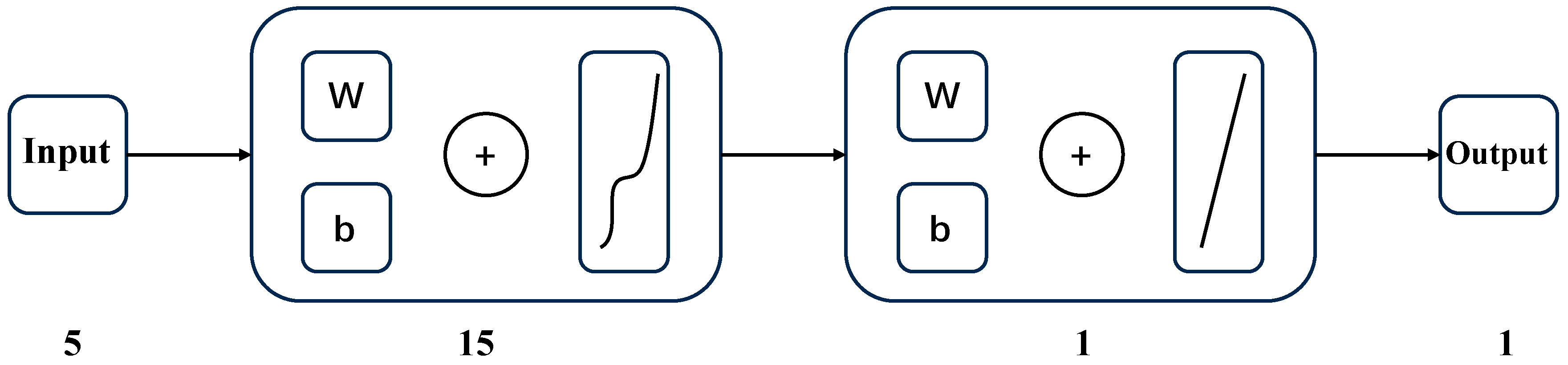
4.2. Establishment of BP Neural Network Model

4.2.1. Input Variables and Output Variables

When studying the solubility of gases in solution, it is important to consider several key factors that significantly affect the dissolution process. According to Henry’s law, pressure is one of the main factors that affects the solubility of gases, and an increase in pressure usually leads to an increase in the solubility of gases in liquids [34]. In addition, temperature also has a significant effect on solubility, and for most gases, an increase in temperature leads to a decrease in solubility due to the fact that the dissolution process is usually accompanied by exothermic heat [35]. Fugacity is also an important influence; it is a parameter that measures the extent to which the actual gas behavior deviates from the ideal gas behavior and has a significant effect on the solubility of the gas in the liquid [36]. In addition, the salinity, i.e., the salt content of the solution, significantly affects the solubility of the gas, and Duan, Møller, and Weare [8] noted that an increase in mineralization leads to a decrease in the solubility of CH₄, which is particularly important in highly saline groundwater or seawater. Finally, the compression factor, a parameter that corrects for non-ideal gas behavior, is particularly critical under high-pressure conditions, and the study by Peng and Robinson [37] provides a useful method for estimating CH₄ fugacity and solubility under different conditions. Therefore, in this paper, pressure and temperature are used as the basis, and then different combinations with salinity, fugacity, and compression factor are formed as input variables to the neural network.

We also consider the effect of hydrate formation on solubility by adjusting the pressure used to calculate the solubility of CH₄ in water when the temperature meets the conditions for hydrate formation.

The solubility S of CH₄ in water is the output variable of the neural network. The solubility S is related to temperature, pressure, salinity, compressibility factor, and fugacity. The output layer contains a neuron unit, which is the solubility S.

4.2.2. Neural Network Training Parameters

The BP artificial neural network comprises an input layer, an output layer, and a crucial intermediate hidden layer. The optimal configuration of this hidden layer, in terms of both the number of layers and nodes, significantly enhances the model’s predictive accuracy. This layer employs a tansig activation function, noted for its smoothness and ease of derivation. The algorithm for the neural network utilizes the Levenberg–Marquardt algorithm, a nonlinear least squares method that combines the strengths of the gradient descent and Gauss–Newton methods. It employs gradients to numerically solve nonlinear minimization. Although increasing the number of hidden layers can improve the network’s function-fitting capability, excessive layers may cause overfitting and complicate data training, hindering model convergence. Furthermore, neural networks are often criticized for their “black box” nature, which means they provide limited transparency and explanations for their decision-making processes.

This paper focuses on establishing the BP neural network model using an intermediate hidden layer with 15 nodes, and the maximum number of training sessions set is 1000. The model’s performance is evaluated using the Mean Relative Error (MRE) between predicted and actual values. The optimal BP neural network model is identified as the one with the input variable that yields the smallest MRE. The input layer data consist of variables such as pressure, temperature, and mineralization levels. Given the diversity of input variables, there are significant differences in the magnitudes and units of these variables. Without preprocessing the input data, the training of the BP neural network would become more challenging and significantly prolong the training duration. Therefore, it is essential to normalize the input data. In this study, the tansig function is used as the activation function for the hidden layers, which necessitates preprocessing all data to fit within the [−1, 1] interval.

4.3. BP Neural Network Prediction

4.3.1. Training Prediction Results for Multiple Combinations of Input Variables

• Temperature, pressure, and salinity (combination 1)

The model incorporates temperature, pressure, and salinity as input variables. Training results, depicted in Figure 7a, show the fluctuation from experimental solubility data, indicating high prediction accuracy. However, the average relative error, as seen in Figure 7b, is 20.86%.

Figure 8a presents the MSE and iteration count during training, revealing a trend where increased iterations enhance alignment with experimental data. The process halts at the 103rd iteration upon reaching acceptable error levels. The green circle in Figure 8a indicates the “best validation performance” position of the model, indicating that the model has the smallest mean square error at the 97th training. Figure 8b displays the correlation coefficients (R) for the training, test, and validation sets, cumulating in a total of 0.97122.

2.

Temperature, pressure, salinity, and compressibility factor (combination 2)

For this model, temperature, pressure, salinity, and compressibility factor serve as inputs. Figure 9a illustrates that the prediction closely matches experimental solubility data, denoting a high degree of model fitting. Figure 9b indicates an improved average relative error of 19.26%, which is more accurate than the previous model.

As detailed in Figure 10a, increasing iterations during training correspond with enhanced predictive accuracy. The process halts at the 39th iteration upon reaching acceptable error levels. The green circle in Figure 10a indicates the “best validation performance” position of the model, indicating that the model has the smallest mean square error at the 39th training. The correlation coefficients, shown in Figure 10b, exhibit an overall improvement with a total of 0.9751.

3.

Temperature, pressure, salinity, and fugacity (combination 3)

This iteration of the model integrates temperature, pressure, salinity, and fugacity. According to Figure 11a, the predictions align well with experimental data, and the model fitting is also superior. Figure 11b notes an average relative error of 21.38%, similar to the previous models.

The training process, including MSE and iteration count, is outlined in Figure 12a. The process halts at the 37th iteration upon reaching acceptable error levels. The green circle in Figure 12a indicates the “best validation performance” position of the model, indicating that the model has the smallest mean square error at the 37th training. The correlation coefficients for various sets are displayed in Figure 12b, with a total of 0.96923.

4.

Temperature, pressure, fugacity, and compressibility factor (combination 4)

Here, the model uses temperature, pressure, enrichment, and compression factor as inputs. Figure 13a shows the difference between the predicted results compared to the experimental data. The average relative error is 35.31%, which is large and indicates that using these four variables as input parameters is not effective, as detailed in Figure 13b.

The training dynamics, shown in Figure 14a, confirm the pattern of increasing accuracy with more iterations. The process halts at the 52nd iteration upon reaching acceptable error levels. The green circle in Figure 14a indicates the “best validation performance” position of the model, indicating that the model has the smallest mean square error at the 52nd training. The overall correlation coefficient, as seen in Figure 14b, is 0.97212.

5.

Temperature, pressure, salinity, fugacity, and compressibility factor (combination 5)

For this comprehensive model, temperature, pressure, salinity, fugacity, and compressibility factor are the inputs. As demonstrated in Figure 15a, the predictions exhibit a high concordance with experimental data. The relative error, shown in Figure 15b, is the lowest among all models at 16.32%, suggesting that the model is the most effective.

Training details, including MSE and iterations, are presented in Figure 16a, and the total correlation coefficient, depicted in Figure 16b, is 0.97401. The green circle in Figure 16a indicates the “best validation performance” position of the model, indicating that the model has the smallest mean square error at the 57th training. The process halts at the 57th iteration upon reaching acceptable error levels.

4.3.2. Selection of the Best CH₄ Gas Solubility Prediction Model

By comparing the results of the five models, the correlation coefficient R of the model with pressure, temperature, compression coefficient, salinity, and fugacity as input variables is 0.97401, which is the best fit, and the average relative error is the smallest among the five models, and the comparison results are shown in

Table 4. Input variables and training results of five models.

Input Variables	MSE	Average Relative Error	Correlation Coefficient R
PTS	4.4106 × 10−5	20.86%	0.97122
PTZF	5.5125 × 10−5	19.26%	0.9751
PTSF	2.4227 × 10−5	21.38%	0.96923
PTZF	3.2585 × 10−5	35.31%	0.97212
PTSZF	4.981 × 10−6	16.32%	0.97401

In the above table, P represents pressure, T represents temperature, S represents salinity, Z represents compression factor, and F represents fugacity.

. Therefore, a BP neural network model was developed using pressure, temperature, compression factor, salinity, and fugacity as input variables and solubility as the output variable. The structure of the BP neural network is shown in Figure 17. Figure 17 shows a four-layer structure including an additional linear layer before the output layer. The fact that this linear layer is part of the network structure does not change the transfer of values from the hidden layer to the output layer. Therefore, this layer can be conceptually omitted.

To enhance the transparency of the neural network model proposed in this paper and to address the issue of traditional neural networks as “black box” models, we have detailed all the weights and bias parameters post-training in Appendix A,

Table A1. Weights and bias parameters of the selected neural network.

Neurons	Input Layer-Hidden Layer Weight P	Input Layer-Hidden Layer Weight T	Input Layer-Hidden Layer Weight S	Input Layer-Hidden Layer Weight Z	Input Layer-Hidden Layer Weight F	Input Layer-Hidden Layer Bias	Output Layer Weights	Output Layer Bias
Neuron 1	−1.13968	−1.76479	−3.45330	1.73109	−3.24137	2.85507	−0.12289	−1.0186
Neuron 2	−0.45666	−7.88603	0.96231	9.97330	0.59206	4.61570	4.61349	−1.0186
Neuron 3	−1.60336	−3.28937	0.26834	3.27836	0.94896	1.70066	−1.23907	−1.0186
Neuron 4	1.01862	1.62973	1.22274	−1.60368	1.00475	−3.64760	3.39638	−1.0186
Neuron 5	0.03258	0.08096	−1.31394	−2.67360	−0.87854	2.14356	1.42482	−1.0186
Neuron 6	−0.17362	−3.31162	−0.56108	0.67030	1.36350	0.53858	−0.55372	−1.0186
Neuron 7	2.97357	1.17050	−0.59135	1.08239	−0.25718	−0.74667	−0.09509	−1.0186
Neuron 8	−1.41132	1.29744	0.77452	1.45754	0.70243	0.91928	−0.01336	−1.0186
Neuron 9	−1.19623	1.18812	−1.38642	0.25159	1.07455	−0.72375	−0.00381	−1.0186
Neuron 10	−1.62494	−1.16618	0.99793	0.21276	1.33450	−1.00104	0.36620	−1.0186
Neuron 11	−0.82606	2.69633	0.31178	−0.70906	−0.86557	−1.89572	−1.21750	−1.0186
Neuron 12	0.86384	1.36316	−1.05806	0.20601	−1.59463	0.36616	0.74156	−1.0186
Neuron 13	1.00624	−0.96938	1.30182	−0.49245	1.47591	1.64634	1.65459	−1.0186
Neuron 14	−1.33706	0.75793	−1.35121	0.47029	−1.37207	−2.08971	1.27833	−1.0186
Neuron 15	0.02949	−1.01606	0.58556	−0.65841	0.42895	2.65211	−2.01326	−1.0186

In the above table, P represents pressure, T represents temperature, S represents salinity, Z represents compression factor, and F represents fugacity.

. This initiative is designed to allow readers to more clearly understand and evaluate the inner workings and decision-making processes of the neural network. By disclosing these critical model parameters, we can thoroughly analyze how the model operates, thereby significantly improving its interpretability and reliability.

Table 5. Mean and standard deviation of input layer weights and biases.

	P	T	S	Z	F	Input Layer-Hidden Layer Bias
average value	1.05	1.97	1.08	1.70	1.14	1.84
standard deviation	0.75	1.87	0.76	2.46	0.70	1.22

shows the mean and standard deviation of the weights and deviations of the input layers. Table 5 indicates that the mean absolute weights of input variables T and Z are higher (1.97 and 1.70, respectively), suggesting these variables have a greater influence on the activation of hidden layer neurons. In contrast, the mean absolute weights of input variables P, S, and F are lower, indicating a relatively weaker effect on hidden layer neurons. The standard deviations of variables Z and T (2.46 and 1.87, respectively) show greater variability across neurons, suggesting the network is more finely tuned to these variables during the training process. Conversely, the smaller standard deviations for variables P, S, and F indicate more consistent weights across neurons. The mean absolute value of the bias from the input layer to the hidden layer is 1.84, with a standard deviation of 1.22. This higher mean value implies that the activation threshold for hidden layer neurons is higher, necessitating larger bias values for activation.

In summary, input variables T and Z exert the most significant influence on hidden layer neurons and exhibit greater variability, suggesting that the network is more responsive to these variables during training. In contrast, variables P, S, and F have less influence and show more consistency. The higher and relatively concentrated bias values indicate a larger bias is required to activate hidden layer neurons. These insights help elucidate the internal mechanisms of the network and provide a basis for further model optimization.

4.3.3. Comparative Analysis of Traditional Methods and Big Data Methods

In this study, a BP neural network was used to predict CH₄ solubility, which was programmed using MATLAB software (R2020b version). The structure of this network consists of an input layer, a hidden layer, and an output layer. The input layer consists of five nodes corresponding to the key variables affecting CH₄ solubility: temperature (T), pressure (P), salinity (S), compression factor (Z), and fugacity (F). The hidden layer is set up as 15 neurons with a hyperbolic tangent (tanh) activation function, a configuration designed to efficiently capture the complex nonlinear relationships among the input variables. The output layer consists of a single neuron that outputs the solubility of CH₄ (S). The network was trained using the Levenberg–Marquardt algorithm, an efficient nonlinear least squares method that combines the advantages of gradient descent and Gauss–Newton methods and is suitable for handling the data size of this study. During the training process, the dataset was randomly divided into a training set (70%) (the data can be viewed at the link in Appendix A), a validation set (15%), and a test set (15%) to evaluate the generalization ability of the model on unseen data. The MSE was used as the performance evaluation metric. To avoid overfitting, training was stopped once the error on the validation set was no longer decreasing, and the model parameters that performed best on the validation set were selected for final testing. All input data were normalized before training to match the input requirements of the activation function. With this refined network configuration and training strategy, the BP neural network model exhibits higher prediction accuracy than the modified Henry’s law over the entire pressure range, reducing the average prediction error to 16.32%, which significantly outperforms the conventional method. This comparison suggests that predictive results derived from big data methodologies surpass those obtained using the modified Henry’s law approach.

A comparison between the predictive results of Henry’s Law and the BP neural network reveals that the BP neural network yields more accurate predictions. This superiority may stem from the empirical nature of Henry’s coefficients, which lack a rigorous theoretical foundation for assessing the impact of varying salinity conditions on CH₄ solubility. Additionally, Henry’s Law does not consider the influence of water vapor in the gas-phase CH₄ on solubility. Consequently, solubility data calculated using the revised Henry’s Law exhibit some discrepancies. In contrast, the BP artificial neural network model effectively addresses complex nonlinear mapping challenges and more accurately correlates solubility with factors such as temperature, pressure, and salinity, making it better suited for these analyses.

Compared with other studies, the computational error in this study is lower than the 23.3% in Sloan’s [38] computation, but higher than the relative error in Hashemi’s [39] computation (<10%), which indicates that there is still room for further optimization of the artificial neural network model in this study.

5. Conclusions

This study integrates Henry’s Law with a BP neural network model to enhance the understanding and prediction of CH₄ gas solubility in water during hydrate formation. We adjusted Henry’s coefficient and employed a BP neural network that considers various influencing factors such as temperature, pressure, and salinity. Our analysis revealed that the BP neural network model outperforms the traditional application of Henry’s Law in predicting gas solubility under varying environmental conditions, mainly due to its superior handling of complex nonlinear relationships.

(1)

We used Henry’s law and a BP neural network model to predict CH₄ solubility, taking into account the effect of hydrates on CH₄ solubility. At the temperature of hydrate formation, the pressure was updated to improve the prediction accuracy of Henry’s law and BP model.

(2)

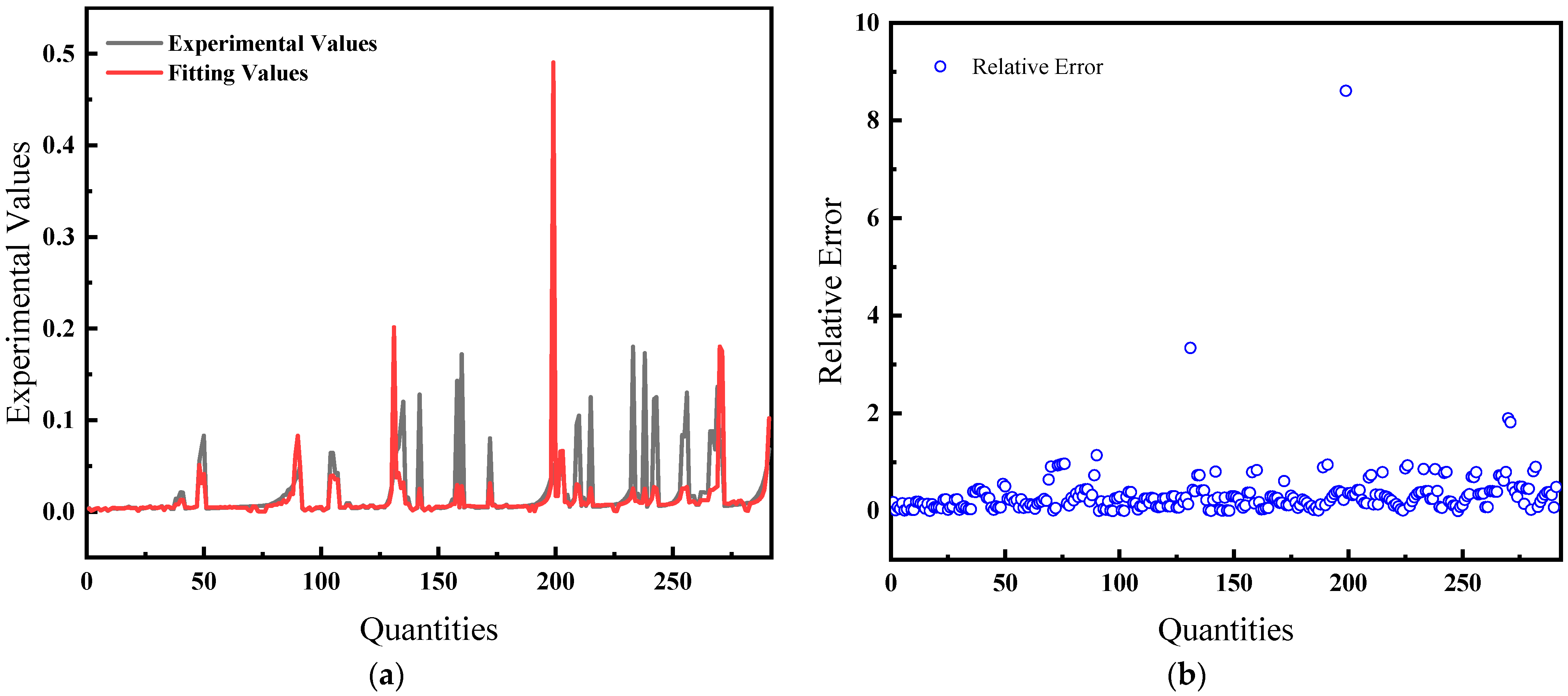
Henry’s coefficient was adjusted, and the solubility of CH₄ gas in water was subsequently calculated using the modified Henry’s Law. The results showed that the model’s predictions were more accurate at lower pressures, with the prediction error increasing at higher pressure states.

(3)

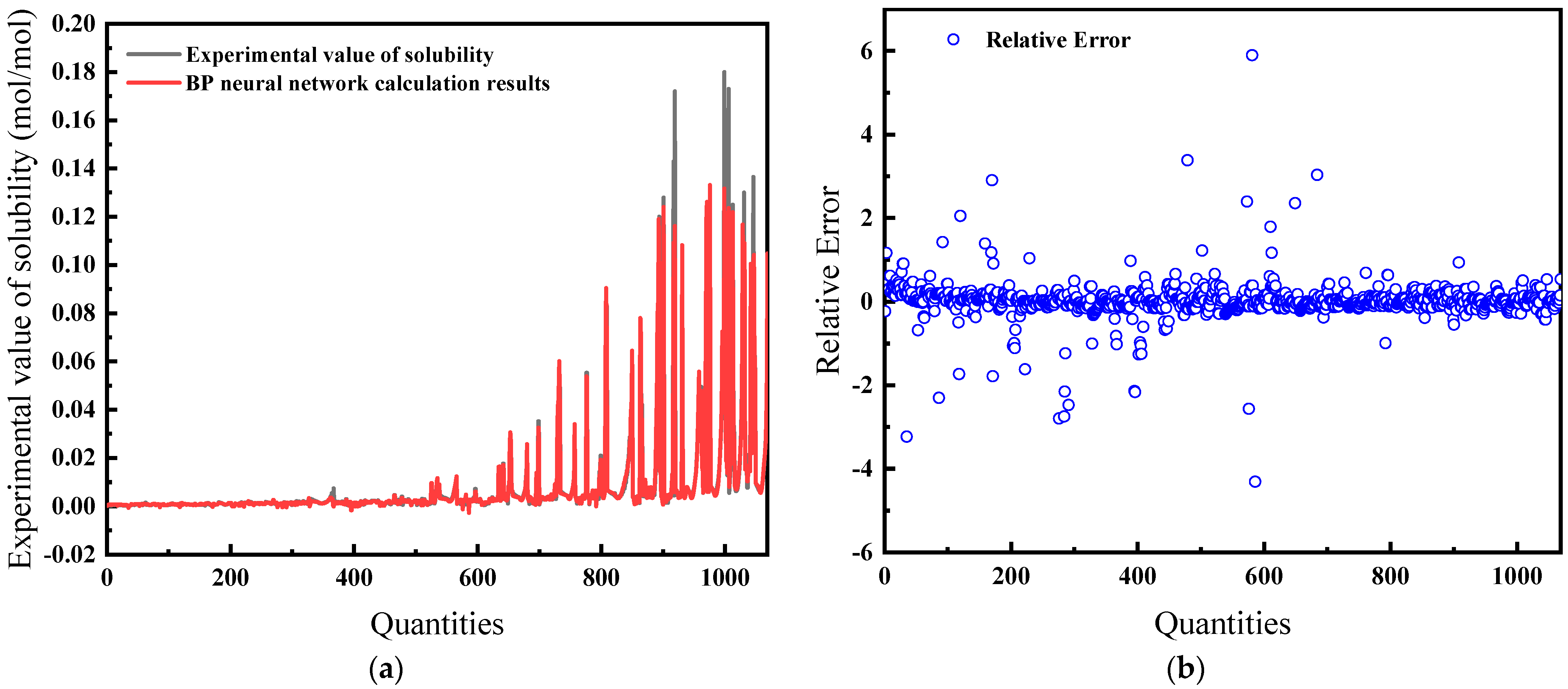
A BP artificial neural network model was developed using solubility data of CH₄ gas in water. By adjusting different input variables for comparison and error analysis, it was ultimately determined that the model with temperature, pressure, salinity, enrichment, and compression factor as input variables was the most effective, with the least error and the best fit.

(4)

We compared the prediction results of Henry’s law and the BP neural network, and the results showed that the neural network model was more accurate for the prediction of CH₄ solubility.

(5)

Despite the progress made, there are still some limitations in this study. First, although the neural network model employed can effectively handle a large range of input variables, its performance and stability under extreme conditions (e.g., very high- or very low-pressure and -temperature conditions) still need to be further verified. In addition, the generalizability and performance of the models in real industrial applications need to be tested more extensively. Secondly, although the model selected in this study has a minimum error of 16.32% in all tests, compared with the models of other scholars, there is still room for further optimization, and attempts can be made to reduce the error in the future by introducing more advanced training algorithms or adjusting the network structure. Finally, the pressure interval selected in this paper is from 1.482 MPa to 120 MPa, and data beyond this range need to be collected to extend the application range of the model and improve its prediction accuracy.

In future work, we will aim to optimize the neural network to improve prediction accuracy under a wider range of environmental conditions.

References

1. Li, L. Solubility and Exsolution Study of CO2 and CH4. Ph.D. Thesis, China University of Geosciences, Beijing, China, 2018. [Google Scholar]
2. Changquan, G. Study of Solubility of Methane in Water Combined With Mechanism of Hydrate Formation. Master’s Thesis, Zhejiang University of Technology, Hangzhou, Zhejiang, 2002. [Google Scholar]
3. Price, L.C. Aqueous Solubility of Methane at Elevated Pressures and Temperatures. AAPG Bull. 1979, 63, 1527–1533. [Google Scholar] [CrossRef]
4. Ou, W.; Geng, L.; Lu, W.; Guo, H.; Qu, K.; Mao, P. Quantitative Raman spectroscopic investigation of geo-fluids high-pressure phase equilibria: Part II. Accurate determination of CH4 solubility in water from 273 to 603 K and from 5 to 140 MPa and refining the parameters of the thermodynamic model. Fluid Phase Equilibria 2015, 391, 18–30. [Google Scholar] [CrossRef]
5. Duffy, J.R.; Smith, N.O.; Nagy, B. Solubility of natural gases in aqueous salt solutions—I: Liquidus surfaces in the system CH4-H2O-NaCl2-CaCl2 at room temperatures and at pressures below 1000 psia. Geochim. Cosmochim. Acta 1961, 24, 23–31. [Google Scholar] [CrossRef]
6. Krader, T.; Franck, E.U. The Ternary Systems H2O-CH4-NaCl and H2O-CH4-CaCl2 to 800 K and 250 MPa. Ber. Bunsenges. Phys. Chem. 1987, 91, 627–634. [Google Scholar] [CrossRef]
7. Hongche, F.; Zhilong, H.; Jian, Y.; Gang, G.; Chuanxin, T.; Chong, F. Methane and carbon dioxide solubility tests under high temperature and pressure conditions. J. China Univ. Pet. (Nat. Sci. Ed.) 2011, 35, 6–11+19. [Google Scholar]
8. Duan, Z.; Møller, N.; Greenberg, J.; Weare, J.H. The prediction of methane solubility in natural waters to high ionic strength from 0 to 250 °C and from 0 to 1600 bar. Geochim. Cosmochim. Acta 1992, 56, 1451–1460. [Google Scholar] [CrossRef]
9. Liang, Y.; Nie, Y. The development of artificial neural network research from the perspective of scientific research methodology. J. Jilin Univ. (Inf. Sci. Ed.) 2002, 1, 59–62. [Google Scholar]
10. Li, M.; Huang, X.; Liu, H.; Liu, B.; Wu, Y.; Xiong, A.; Dong, T. Prediction of gas solubility in polymers by back propagation artificial neural network based on self-adaptive particle swarm optimization algorithm and chaos theory. Fluid Phase Equilibria 2013, 356, 11–17. [Google Scholar] [CrossRef]
11. Mohammadi, M.-R.; Hadavimoghaddam, F.; Atashrouz, S.; Abedi, A.; Hemmati-Sarapardeh, A.; Mohaddespour, A. Modeling the solubility of light hydrocarbon gases and their mixture in brine with machine learning and equations of state. Sci. Rep. 2022, 12, 14943. [Google Scholar] [CrossRef]
12. Taherdangkoo, R.; Liu, Q.; Xing, Y.; Yang, H.; Cao, V.; Sauter, M.; Butscher, C. Predicting methane solubility in water and seawater by machine learning algorithms: Application to methane transport modeling. J. Contam. Hydrol. 2021, 242, 103844. [Google Scholar] [CrossRef]
13. Deng, H.; Guo, Y. Artificial Neural Network Model for the Prediction of Methane Bi-Reforming Products Using CO2 and Steam. Processes 2022, 10, 1052. [Google Scholar] [CrossRef]
14. Li, T.; Tantikhajorngosol, P.; Yang, C.; Tontiwachwuthikul, P. Experimental investigations and developing multilayer neural network models for prediction of CO2 solubility in aqueous MDEA/PZ and MEA/MDEA/PZ blends. Greenh. Gases Sci. Technol. 2021, 11, 712–733. [Google Scholar] [CrossRef]
15. Hamzehie, M.E.; Mazinani, S.; Davardoost, F.; Mokhtare, A.; Najibi, H.; Van der Bruggen, B.; Darvishmanesh, S. Developing a feed forward multilayer neural network model for prediction of CO2 solubility in blended aqueous amine solutions. J. Nat. Gas Sci. Eng. 2014, 21, 19–25. [Google Scholar] [CrossRef]
16. Mokarizadeh, H.; Atashrouz, S.; Mirshekar, H.; Hemmati-Sarapardeh, A.; Mohaddes Pour, A. Comparison of LSSVM model results with artificial neural network model for determination of the solubility of SO2 in ionic liquids. J. Mol. Liq. 2020, 304, 112771. [Google Scholar] [CrossRef]
17. Mohammadi, M.-R.; Hadavimoghaddam, F.; Atashrouz, S.; Abedi, A.; Hemmati-Sarapardeh, A.; Mohaddespour, A. Toward predicting SO2 solubility in ionic liquids utilizing soft computing approaches and equations of state. J. Taiwan Inst. Chem. Eng. 2022, 133, 104220. [Google Scholar] [CrossRef]
18. Prausnitz, J.M.; Lichtenthaler, R.N.; Azevedo, E.G.D. Molecular Thermodynamics of Fluid-Phase Equilibria; Prentice-Hall: Upper Saddle River, NJ, USA, 1999. [Google Scholar]
19. Böttger, A.; Pérez-Salado Kamps, Á.; Maurer, G. An experimental investigation of the phase equilibrium of the binary system (methane+water) at low temperatures: Solubility of methane in water and three-phase (vapour + liquid + hydrate) equilibrium. Fluid Phase Equilibria 2016, 407, 209–216. [Google Scholar] [CrossRef]
20. Rahmati-Abkenar, M.; Manteghian, M. Effect of silver nanoparticles on the solubility of methane and ethane in water. J. Nat. Gas Sci. Eng. 2020, 82, 103505. [Google Scholar] [CrossRef]
21. Wang, L.-K.; Chen, G.-J.; Han, G.-H.; Guo, X.-Q.; Guo, T.-M. Experimental study on the solubility of natural gas components in water with or without hydrate inhibitor. Fluid Phase Equilibria 2003, 207, 143–154. [Google Scholar] [CrossRef]
22. Kiepe, J.; Horstmann, S.; Fischer, K.; Gmehling, J. Experimental Determination and Prediction of Gas Solubility Data for Methane + Water Solutions Containing Different Monovalent Electrolytes. Ind. Eng. Chem. Res. 2004, 43, 3216. [Google Scholar] [CrossRef]
23. Zhao, G.; Gong, G.; Sun, H.; Chen, B.; Zheng, J.-N.; Yang, M. Effect of Methane Solubility on Hydrate Formation and Dissociation: Review and Perspectives. Energy Fuels 2022, 36, 7269–7283. [Google Scholar] [CrossRef]
24. Michels, A.; Gerver, J.; Bijl, A. The influence of pressure on the solubility of gases. Physica 1936, 3, 797–808. [Google Scholar] [CrossRef]
25. O’sullivan, T.D.; Smith, N.O. Solubility and partial molar volume of nitrogen and methane in water and in aqueous sodium chloride from 50 to 125.deg. and 100 to 600 atm. J. Phys. Chem. 1970, 74, 1460–1466. [Google Scholar] [CrossRef]
26. Amirijafari, B.; Campbell, J.M. Solubility of Gaseous Hydrocarbon Mixtures in Water. Soc. Pet. Eng. J. 1972, 12, 21–27. [Google Scholar] [CrossRef]
27. Crovetto, R.; Fernández-Prini, R.; Japas, M.L. Solubilities of inert gases and methane in H2O and in D2O in the temperature range of 300 to 600 K. J. Chem. Phys. 1982, 76, 1077–1086. [Google Scholar] [CrossRef]
28. Aggarwal, C.C. Outlier Analysis; Springer: New York, NY, USA, 2013. [Google Scholar]
29. Pyle, D. Data Preparation for Data Mining; Elsevier Science: Amsterdam, The Netherlands, 1999. [Google Scholar]
30. Vul’fson, A.N.; Borodin, O.O. A thermodynamic analysis of the solubility of gases in water at high pressures and supercritical temperatures. Russ. J. Phys. Chem. A 2007, 81, 510–514. [Google Scholar] [CrossRef]
31. Englezos, P.; Bishnoi, P.R. Gibbs free energy analysis for the supersaturation limits of methane in liquid water and the hydrate-gas-liquid water phase behavior. Fluid Phase Equilibria 1988, 42, 129–140. [Google Scholar] [CrossRef]
32. Song, K.Y.; Feneyrou, G.; Fleyfel, F.; Martin, R.; Lievois, J.; Kobayashi, R. Solubility measurements of methane and ethane in water at and near hydrate conditions. Fluid Phase Equilibria 1997, 128, 249–259. [Google Scholar] [CrossRef]
33. Carroll, J.J.; Mather, A.E. A model for the solubility of light hydrocarbons in water and aqueous solutions of alkanolamines. Chem. Eng. Sci. 1997, 52, 545–552. [Google Scholar] [CrossRef]
34. Sander, R. Compilation of Henry’s law constants (version 4.0) for water as solvent. Atmos. Chem. Phys. 2015, 15, 4399–4981. [Google Scholar] [CrossRef]
35. Lide, D.R. CRC Handbook of Chemistry and Physics; CRC press: Boca Raton, FL, USA, 2004; Volume 85. [Google Scholar]
36. Duan, Z.; Sun, R. An improved model calculating CO2 solubility in pure water and aqueous NaCl solutions from 273 to 533 K and from 0 to 2000 bar. Chem. Geol. 2003, 193, 257–271. [Google Scholar] [CrossRef]
37. Peng, D.-Y.; Robinson, D.B. A new two-constant equation of state. Ind. Eng. Chem. Fundam. 1976, 15, 59–64. [Google Scholar] [CrossRef]
38. Sloan, E.; Koh, C. Clathrate Hydrates of Natural Gases; Marcel Decker. Inc.: New York, NY, USA, 1998. [Google Scholar]
39. Hashemi, S.; Macchi, A.; Bergeron, S.; Servio, P. Prediction of methane and carbon dioxide solubility in water in the presence of hydrate. Fluid Phase Equilibria 2006, 246, 131–136. [Google Scholar] [CrossRef]
Figure 1. Solubility of CH4 in water [4]: (a) 273.15–373.15 K; (b) 433.15–603.15 K.
Processes 12 01091 g001
Figure 2. Solubility of CH4 in 315.9 g/L NaCl solution [24].
Processes 12 01091 g002
Figure 3. CH4 hydrate formation curve.
Processes 12 01091 g003
Figure 4. Comparison of predicted and actual values and average relative errors for pressures less than or equal to 40 MPa: (a) Comparison of fitting values with experimental values; (b) Relative error between fitting and experimental values.
Processes 12 01091 g004
Figure 5. Comparison of predicted and actual values and average relative errors for pressures greater than 40 MPa: (a) Comparison of fitting values with experimental values; (b) Relative error between fitting and experimental values.
Processes 12 01091 g005
Figure 6. Basic structure of BP neural network.
Processes 12 01091 g006
Figure 7. Comparison of predicted results and Relative Error for combination 1: (a) BP network predicted value and experimental value; (b) Relative error between BP network predicted value and experimental value.
Processes 12 01091 g007
Figure 8. Comparison of predicted results and Relative Error for combination 1: (a) MSE varies with the number of iterations; (b) Correlation coefficient R.
Processes 12 01091 g008
Figure 9. Comparison of predicted results and Relative Error for combination 2: (a) BP network predicted value and experimental value; (b) Relative error between BP network predicted value and experimental value.
Processes 12 01091 g009
Figure 10. Comparison of predicted results and Relative Error for combination 2: (a) MSE varies with the number of iterations; (b) Correlation coefficient R.
Processes 12 01091 g010
Figure 11. Comparison of predicted results and Relative Error for combination 3: (a) BP network predicted value and experimental value; (b) Relative error between BP network predicted value and experimental value.
Processes 12 01091 g011
Figure 12. Comparison of predicted results and Relative Error for combination 3: (a) MSE varies with the number of iterations; (b) Correlation coefficient R.
Processes 12 01091 g012
Figure 13. Comparison of predicted results and Relative Error for combination 4: (a) BP network predicted value and experimental value; (b) Relative error between BP network predicted value and experimental value.
Processes 12 01091 g013
Figure 14. Comparison of predicted results and Relative Error for combination 4: (a) MSE varies with the number of iterations; (b) Correlation coefficient R.
Processes 12 01091 g014
Figure 15. Comparison of predicted results and Relative Error for combination 5: (a) BP network predicted value and experimental value; (b) Relative error between BP network predicted value and experimental value.
Processes 12 01091 g015
Figure 16. Comparison of predicted results and Relative Error for combination 5: (a) MSE varies with the number of iterations; (b) Correlation coefficient R.
Processes 12 01091 g016
Figure 17. The BP neural network structure of this paper.
Processes 12 01091 g017