Abstract
Renewable sources of energy production are some of the main targets today to protect the environment through reduced fossil fuel consumption and CO2 emissions. Alongside wind, solar, marine, biomass and nuclear sources, hydropower is among the oldest but still not fully explored renewable energy sources. Compared with other sources like wind and solar, hydropower is more stable and consistent, offering increased predictability. Even so, it should be analyzed considering water flow, dams capacity, climate change, irrigation, navigation, and so on. The aim of this study is to propose a forecast model of hydropower production capacity and identify long-term trends. The curve fit forecast parabolic model was applied to 33 European countries for time series data from 1990 to 2021. Space-time cube ArcGIS representation in 2D and 3D offers visualization of the prediction and model confidence rate. The quadratic trajectory fit the raw data for 14 countries, validated by visual check, and in 20 countries, validated by FMRSE 10% threshold from the maximal value. The quadratic model choice is good for forecasting future values of hydropower electric capacity in 22 countries, with accuracy confirmed by the VMRSE 10% threshold from the maximal value. Seven local outliers were identified, with only one validated as a global outlier based on the Generalized Extreme Studentized Deviate (GESD) test at a 5% maximal number of outliers and a 90% confidence level. This result achieves our objective of estimating a level with a high degree of occurrence and offering a reliable forecast of hydropower production capacity. All European countries show a growing trend in the short term, but the trends show a stagnation or decrease if policies do not consider intensive growth through new technology integration and digital adoption. Unfortunately, Europe does not have extensive growth potential compared with Asia–Pacific. Public policies must boost hybrid hydro–wind or hydro–solar systems and intensive technical solutions.
1. Introduction
Today, society faces multiple radical transformations in all social and economic aspects, acting individually but also interconnected, determining complex synergies [1]. The shift towards renewable energy sources represents one of the most significant transformations in the 21st-century global energy landscape. This transition is not merely a change in energy types used; it is a profound evolution touching upon economic policies, technological advancements, environmental considerations, and societal well-being. At its core, the shift to renewable energy sources is driven by the urgent need to reduce fossil fuel usage, considered the highest polluter, and minimize CO2 emissions. Renewable energy sources, including solar, wind, hydroelectric, and geothermal power, offer a cleaner alternative, producing little to no greenhouse gas emissions during operation. By harnessing the power of nature, renewable energy can provide electricity, heating, and transportation without depleting our planet’s resources or harming its ecosystems. This transition not only addresses the immediate challenges of climate change but also underscores a commitment to environmental stewardship and preserving of the planet for future generations.
Economic considerations and technological innovations also drive the shift to renewable energy. The cost of renewable energy technologies has decreased in recent years, making them increasingly competitive with traditional fossil fuels. Solar and wind power have seen dramatic reductions in cost due to advancements in technology and increased production scale. This cost competitiveness, coupled with government policies and incentives to support renewable energy, has accelerated the deployment of renewable energy projects worldwide. Furthermore, the transition to renewable energy sources presents significant economic opportunities, including job creation in new industries, reduced energy costs for consumers, and the potential for technological leadership on the global stage. Countries and companies that invest in renewable energy technologies stand to benefit from the growing global demand for clean energy solutions, positioning themselves as leaders in a rapidly evolving energy market. Compared with solar and wind energy, which are highly dependent on weather, hydropower production capacity is less sensitive to the climate and more constant.
Renewable energy sources are abundant and widely distributed geographically, reducing risks associated with geopolitical tensions and supply disruptions. Countries can enhance their energy independence by investing in renewable energy and ensuring a more stable and secure energy supply. The potential of natural resources and power production capacity should be explored to design the energy mix and secure a constant power supply for individuals and companies.
The European Commission recently underscored that over 75% of EU greenhouse gas emissions are attributed to energy production and consumption [2]. Consequently, decarbonizing the EU’s energy system is crucial to meeting our 2030 climate goals and attaining the Union’s goal of carbon neutrality by 2050. This acknowledgment has set in motion an irreversible transformation of the economies within EU member states. In line with the [3] and the Framework Strategy for a Resilient Energy Union with a Forward-Looking Climate Change Policy [4], the EU27 has outlined its action plan along five key dimensions: energy security, decarbonization, energy efficiency, the internal energy market, and research, innovation, and competitiveness. The renewable energy sector plays a pivotal role in this economic transformation. This commitment is mirrored in the Green Deal’s [2] target of achieving a 32% share of renewable energy consumption by 2030.
Hydropower energy production for the year 2022 [5] was 4334.19 Tera Watts/hour, compared with 3430.13 TWh in 2010, 2646.73 TWh in 2000, and 1731.65 TWh in 1980. The regional shares are presented in Figure 1.

Figure 1.
Regional shares of hydropower production, 2022 [5]; Source: authors’ representation.
While global hydropower production growth has been 150% over the last 42 years, it has been only 22% for Europe and 599% for Asia–Pacific. Based on these statistics, knowing the hydropower production potential and trends is essential for decision makers and the reliability of renewable sources.
The need for renewable energy is growing, and hydropower plays an important role because of its advantages compared with other renewable sources. The proposed model used a big data package to identify the hydropower production capacity’s parabolic curve evolution with a high accuracy rate. The forecast for 2022–2025 provides valuable insight into how much EU countries can count on hydropower individually and regionally. The most important contribution of the present study is to provide at least a partial answer to the question: Is hydropower the solution for the renewable energy shift in Europe? The global picture offered by our findings is a pillar of energy strategies for the European Union and each European country and could be replicated for other regions.
Forecasting hydropower production capacity is crucial for several reasons, all contributing to the efficient and sustainable management of energy resources. As the world transitions towards renewable energy to combat climate change, understanding hydropower’s future potential and limitations is essential. Here is a detailed explanation of the need for such forecasts:
- Energy Planning and Policy Making: Accurate forecasts of hydropower production capacity enable governments and energy planners to make informed decisions about future energy policies and infrastructure investments. Hydropower, a significant component of renewable energy portfolios, requires strategic planning to ensure it complements other energy sources. Forecasts help determine the optimal mix of energy sources, thereby enhancing energy security and reliability;
- Grid Stability and Management: Hydropower plants often play a crucial role in maintaining grid stability due to their ability to quickly ramp up and down production in response to fluctuating demand. By forecasting hydropower capacity, grid operators can better manage the balance between supply and demand, preventing blackouts and ensuring a stable electricity supply. This is particularly important as grids increasingly incorporate variable renewable energy sources like wind and solar power;
- Water Resource Management: Hydropower production is closely linked to water availability, which is subject to seasonal and annual variations. Forecasting helps in the effective management of water resources, ensuring that water storage and release schedules from reservoirs are optimized for power generation and other uses, such as irrigation, flood control, and potable water supply. This is especially critical in regions experiencing water scarcity or competing water demands;
- Climate Change Adaptation: Climate change significantly impacts precipitation patterns, snowmelt, and river flows, affecting hydropower production. Forecasting allows for the anticipation of these changes and the development of adaptive strategies to mitigate adverse effects. These strategies might include modifying operational protocols, enhancing reservoir capacity, or investing in climate-resilient infrastructure;
- Economic Efficiency: Hydropower is a capital-intensive investment, and its economic viability depends on consistent and predictable power generation. Accurate forecasts allow for better financial planning and risk management, giving investors and stakeholders confidence to support long-term hydropower projects. They also aid in setting competitive electricity tariffs, benefiting producers and consumers;
- Environmental Protection: Forecasting hydropower capacity helps minimize the environmental impact of power generation. By optimizing the timing and quantity of water releases, downstream ecosystems and biodiversity can be protected. Additionally, forecasts can aid in planning for fish migration and other ecological considerations often affected by hydropower operations;
- Integration with Other Renewables: As the share of renewable energy increases in the energy mix, hydropower can serve as a reliable backup to intermittent sources like wind and solar. Forecasting hydropower capacity enables better integration and coordination with these sources, ensuring a stable and continuous power supply. This hybrid approach leverages the strengths of different renewable technologies, maximizing overall system efficiency and resilience.
In summary, forecasting hydropower production capacity is essential for efficient energy planning, grid stability, water resource management, climate change adaptation, economic efficiency, environmental protection, and the integration of renewables. It equips policymakers, grid operators, and investors with the insights needed to navigate the complexities of energy production and resource management in a rapidly changing world. As such, it is a critical tool in pursuing sustainable and resilient energy systems.
The overall contribution of the present study is the integrated X-ray picture of the hydropower production capacity in the European Union and the trends and forecasts for the upcoming years. This basic pillar is the evidence base for the restructuring strategies of the energy mix and the shift from fossil fuel to renewable energy source policies. The change from fossil fuel, a stored type of energy, to renewable energy sources, a runoff energy type, is challenging for decision makers due to the uncertainty and unpredictability of production. Moreover, the forecast and trends of hydropower production capacity, the most stable source compared with wind and solar, establish the main lines of the strategies for innovation and technological development of the hydropower sector, digital adoption, skilling, and reskilling of human resources. This subject carries significant implications for multiple facets of society, including the economy, environmental protection, labor market, education, and overall standard of living. It underscores the ongoing structural transformation of economies towards sustainability, leading to the emergence of new economic sectors while phasing out others. This transition necessitates substantially reallocating the labor force, not just within sectors but notably between them. The shift towards green foundations amplifies the complexity of this process, accentuating the need for comprehensive strategies to navigate these changes effectively and ensure sustainable growth and prosperity. Based on this study and the findings, an integrated, interdisciplinary, and complex scientific construction can be developed, offering real-life operators the best support for their long-term strategic vision.
The novelty of the proposed model is, firstly, the novelty of the tools used. The SMART data use is represented by the NetCDF data formats for both the input and output of the model. Our data are structured in a Space-Time Cube data cube by generating space-time bins with defined features and associated spatiotemporal attributes. This fact is highly important for the high level of data interoperability with machines (i.e., interfaces for C, C++, Java, Python, IDL, MATLAB, R, Ruby, and Perl, etc.). Secondly, there is a high potential to apply a large spectrum of forecasting tools, which are more complex and differentiated by the assumption of seasonality modeling, from the simplest hypothesis to the more complex one. This study explores the natural trend of hydropower production capacity and generates a forecast based on the assumption of non-seasonal variation modeling with the simplest forecast tool (Curve Fit Forecast) as a first step in the new digital era of SMART data. Forecasting entails using historical data and statistical techniques to predict future events or trends. Scrutinizing patterns and trends in previous data enables making educated predictions about what may occur in the future. From this perspective, the study proceeds, for the first time, with data from 32 years and 33 locations. Thirdly, the combination of the Curve Fit Forecast with the New Space-Time Pattern Mining Tools and the Visualized Space-Time Cube in 2D and 3D, using NetCDF data, gives better insight and accessible information to decision makers. A tendency to specialize in hydropower production capacity can be identified in our case, as well as the less extensive capacity development.
2. Background Literature
Next year, the European Union aims to replace fossil fuels with renewable energy. Hydropower is one of the oldest energy sources, especially watermills, and the well-known Dutch windmills for wind. The motivation to focus on renewable energy is less pollution and spoiling of resources, despite the lower technology costs and regional dependencies [6]. The cohesion between energy and the environment must be mitigated to reach the optimal balance between power generation and environmental protection [7].
Small producers are equally important as large ones and consistently contribute to power generation for regions with large river structures [8]. The shift from fossil fuels to renewable energy is a challenge if economic development is to be sustained [9].
Hydropower production is more stable than wind and solar, and the need for storage is less in the short term. Once the other regenerative sources become more productive, hydropower will maintain the balance [10].
To establish the efficiency of hydropower production, interdisciplinary studies should be conducted; hydrologic flow and climate change influence hydropower production [11,12] The small-scale production of hydropower generates consistent extensive growth and gains a large share of the total; its fluctuation must be evaluated using hydrologic flow and other influencing factors such as irrigation and water supply [13,14]. Other studies, besides hydrology and hydrogeology are considered to estimate the efficiency and opportunity of hydropower development [15].
Manzano-Agugliaro et al. [16] explored small-scale hydropower installation and potential in European countries, highlighting Italy, Austria, Greece, Spain, and France with over 4000 GWh potential. The estimated worldwide potential of small-scale hydropower [17,18] shows the highest for Asia–Pacific (3.73 PWh) and lowest for Europe (0.34 PWh), but still a considerable quantity to be developed. The production must be correlated with storage and water supply for sustainable exploitation and conservation of the resources [19]. Dam construction could contribute to river flow optimizations and regional development, but it could also imbalance the environment [20]; sustainable solutions must be considered according to local conditions [21,22]. The last decade has been characterized by explosive dam construction [23], with Southern Europe representing a hotspot [24]. Moreover, forecasting hydropower in a dam network optimizes the production capacity [25].
Integrated power generation systems using different sources are a better solution than relying on a single option; wind and hydropower have synergy and flexibility [26,27]. Small hydropower production can be combined with solar energy. Kougias et al. [28] studied complementarity, revealing a need for stimulating multi-source compromise. These new systems integrate technical solutions that are more flexible and sensitive to water flow changes and storage solutions [29].
Energy public policies consider all local resources and the complementarity of renewable energy sources with projects like water supply, irrigation, navigation, and recreation facilities to create the best combination [30,31]. The opportunity for small-scale hydropower in Malaysia [32] identifies considerable potential with only 17.5% capacity installed. Energy production has to be balanced with the environmental conditions for each location to avoid damaging the ecosystem [33].
A model of an integrated energy system is proposed for South and Central America by Barbosa et al. [34], covering the local potential and storage facilities. The local resources are influenced by the season, and the complementarity of the sources should cover them [35]. The analysis of the Swiss Cantons’ uses of small-scale hydropower [36] argues for considering regional and local factors and mixed energy policies. Creating a renewable energy mix requires a multicriterial model that considers the sensitivity analysis and the sources’ complementarity [37,38]. Small-scale hydropower sources are highly appreciated as a mass local sustainable solution. Drakaki et al. [39] propose a day-ahead forecast for a small hydro plant to reveal its potential or hydropower scheduling [40]. Jurasz et al. [41] developed a day-ahead model for a hydro–wind hybrid system.
The efficiency of hydropower production depends not only on the water flow but also on the technology used. Hatata et al. [42] compared three types of turbines for small hydropower in Egypt and found that Crossflow and Kaplan are suitable solutions. A comprehensive study [43] on digital adoption in hydropower production and storage makes it a more versatile and efficient replacement for fossil fuel; unfortunately, the potential is extensively limited, so the orientation is to make it intensively unlimited.
Zhou et al. [44] developed a forecast model (DeepHydro) for hydropower production for a river with multiple stations, and Rahman et al. [45] developed a prediction methodology using artificial neural networks. Similarly, cascade hydropower can be estimated [46] or a hybrid hydro-photovoltaic system [47]. The study [45] presented power forecasting methods for solar, wind, and hydro sources using artificial neural networks. The forecasting models [48,49,50,51,52] refer to the power forecast of a location with influence factors. The multi-criteria factors forecast for a dam reservoir gives a hint about the sustainable exploitation of the hydrologic resources [53]. Bernardes et al. [54] reviewed the studies that present machine learning in hydropower production and clustered them. The findings show a large area of applications (supervising, operation management, river flow, etc.) and propose another area to be explored [55,56]. Machine learning is used by Sapitang et al. [57] to forecast the changes in water in a hydropower supplier reservoir. Sweeney et al. [58] also proposed a framework model for wind and solar energy forecasting. Another type of forecasting is for renewable energy for one country (e.g., Poland) to estimate the energy mix [59,60,61,62].
Pata and Aydin [63] tested the environmental Kuznets curve to evaluate the ecological footprint of the six hydropower producers (Brazil, China, Canada, India, Norway, and the USA). Unfortunately, the model does not confirm the beneficial effects, and other renewable energies should be considered.
The forecast of the hybrid renewable sources combines hydropower production and relative stability with solar and wind to obtain optimal storage and cost results [27,64,65,66].
Considering the strategic context and the target of the Green transition, which implies the energy transition from fossil fuel to renewable sources without economic deceleration and electric power consumption growth, all actors are paying attention to the potential implementation direction. Knowing the most promising renewable sources in terms of capacity development, yield, predictability, and availability for digital adoption and innovation, the best strategic frameworks can be set up. The X-ray analysis of the actual stage, combined with trends and perspective, depicts the best pathways of this radical transition nowadays. The forecast subject was of interest to scientists looking for solutions to reach the optimum in renewable energy production, especially in hydropower. So far, the worldwide potential of hydropower production capacities, dams or dam systems/cascades, river systems, countries’ resources, and hybrid systems has been explored. No study was dedicated to European countries, and no curve fit forecast was used before. Moreover, the identified gap in the literature is the countries’ forecast on short-term and long-term trends. To address it, the following hypotheses were set up:
Hypothesis 1:
The curve fit parabolic forecast model gives a reliable approximation of the hydropower production capacity (1990–2021).
Hypothesis 2:
The hydropower production capacities are on an uptrend for the period 1990–2025 in all European countries.
Hypothesis 3:
Countries’ capacity to produce electrical hydropower differs by speed and acceleration.
Hypothesis 4:
The quadratic model validates for all 33 European countries the medium-term level forecast of hydropower production capacities.
Hypothesis 5:
How many outliers does the data set contain?
3. Materials and Methods
MW’s net maximum electrical capacity is the main technical characteristic of plants that produce electrical energy from hydro sources, which this study calls hydropower production capacities.
Green energy production is a priority in implementing the Green Transition. Implementing this objective requires an objective assessment, first of all, of the resources involved in this process. Thus, the first essential stage is the analysis of the natural trend of the evolution of the hydropower production capacity in the well-known context of the dependence on the geographical resources that allow the exploitation of the potential energy of water. Hydropower production capacity depends on static characteristics such as water basins and dynamic characteristics, respectively, on the amount and flows of water that feed the water basins. For the first time, we propose a space-time analysis of the hydropower production capacity in annual variation for the European countries over three decades, a fact that requires an integrated analysis using the latest tools.
The novelty of the tools used in the construct of the study is the data engineering under space-time format managed as Space-Time Cube in NetCDF data formats, an array-oriented scientific data format in trend with the New Data Revolution. The “classical” panel data from Eurostat were transformed into NetCDF data, which means that these new forms of data use software libraries and machine-independent data formats that support the creation, access, and sharing. The advantages of data in netCDF format are that these data are self-describing, portable, scalable, appendable, sharable, and archivable. That is why the first result of the study is the valuable input and output NetCDF data creation.
Moreover, the hydropower production capacity forecast as a non-seasonal process was modelled with the Curve Fit Forecast tool launched since 2020 in ArcGIS PRO Spatial Statistical Tool, which reconfirms the novelty and complexity of the methods.
Forecast methods need consistent time series for much shorter time predictions. Using a time series for a period of 32 years, the authors applied the Curve Fit Forecast tool. It approximates the curve to predict the future values for each location in a space-time cube [67]. Various curves are considered for the forecast: parabolic, exponential, or S-shape (Gompertz). For this study, the parabolic curve was selected to forecast the hydropower production capacity in the EU countries as the best, in our opinion, to identify the uptrends and downtrends of the hydropower production capacity. The Curve Fit Forecast tool uses curve fitting to predict future values for each location within a space-time cube. Initially, the tool fits a parametric curve to each location in the Input Space-Time Cube; subsequently, it forecasts the time series by extending this curve to future time steps [68].
The general working assumptions of the model are:
- (a)
- Hydropower production capacity is predictable;
- (b)
- The annual data of the hydropower production capacity are not affected by seasonality, a fact that indicates a simplified trend;
- (c)
- Curve Fit Forecast is a proper modeling tool that lends itself to process data not affected by seasonality;
- (d)
- The simple trend of the data led us to use the Curve Fit Forecast tool as the most suitable tool from the package available in the ArcGIS Time Series Forecasting toolset. Exponential Smoothing Forecasts moderate trends and strong seasonal behavior [68] (Buie, 2020), and Forest-based Forecast is used when the data exhibits intricate trends or seasonal patterns or undergoes changes that do not conform to typical mathematical functions like polynomials, exponential curves, or sine waves [69] (Esri, 2023).
On the other hand, a forecast involves projecting future developments but with a certain level of uncertainty due to external factors that may impact the outcome according to Seradayan et al. [70].
The Curve Fit Forecast method stands out because it fits various parametric curves to data, handles non-linear trends, and manages multivariate spatial-temporal datasets. Its integration with GIS platforms and advanced computational techniques makes it a powerful tool for modern data analysis and forecasting. As data grow in volume and complexity, the Curve Fit Forecast method offers a novel and sophisticated approach to making accurate and reliable predictions, essential for informed decision making in numerous fields.
3.1. Quadratic Time Model
The parabolic equation of the variation of hydropower production capacity, according to Galileo’s equation, under the assumption of rectilinear and uniform movement over time. The general form of the equation is:
where is a Curve-Fit Parabolic Forecast, is the quadratic component, is the linear component, c is the constant, a is the quadratic coefficient, and b is the linear coefficient. It is very important to emphasize that the Curve-Fit Forecast, the Exponential Smoothing Forecast, and the Forest-based Forecast represent a set of advanced statistical techniques introduced in the Spatial Statistics Package in December 2020 as part of the ArcGIS Pro 2.7 release [71] (Bakshi, 2020).
The transposition of the Equation (1) for the hydropower production capacity is:
where is the hydropower production capacity for a location (i = 1, 2, …33), a is the quadratic coefficient, b is the linear coefficient, c is the constant, and t is the time. Considering the interpretation of the hydropower production capacity at constant acceleration, respectively only its speed changes in time, according to parabolic kinematic, ignoring the cause of this variation, then acceleration (acc) is 2a, and b is the linear coefficient like the initial velocity. The kinematics equations for the hydropower production capacity follow the uniformly accelerated rectilinear motion model, also known as constant acceleration motion.
Velocity and acceleration are the concepts used to interpret the model results. Velocity is a vector quantity that describes the rate at which an object covers distance. Velocity indicates how fast an object is moving, regardless of its direction. Acceleration is a vector quantity that describes the rate of velocity change with respect to time. It indicates how quickly an object’s velocity is changing. Acceleration can occur in various directions, including increasing and decreasing velocity. Positive acceleration indicates speeding up, while negative acceleration (also known as deceleration or retardation) indicates slowing down.
The model performance is measured using the Root Mean Square Error (RMSE). RMSE is an accuracy metric useful for evaluating forecasting errors across various models on the same dataset rather than across different datasets due to its scale sensitivity. It is always a non-negative value, with 0 being the ideal but practically unattainable figure, signifying a perfect match with the data. Generally, a smaller RMSE value is preferable, indicating a closer fit to the observed data. Nonetheless, comparing different datasets is not appropriate, as the scale of the data involved influences RMSE values [72]. RMSE is optimal for normal (Gaussian) errors [73].
3.2. Forecasting Model or Evaluate the Curve to Fit with the Raw Data
A curve was generated using an econometric model of the parabolic type for the forecast model. Forecasting the RMSE value allows us to see how well the estimated curve fits the original data, or in other words, how much the curve differs from the raw data. For this purpose, at each location of the space-time cube, the square root of the average squared difference between the curve (ct) and the raw values of the time series (rt) was measured for all time series bins (see Equation (3)).
where T is the number of time steps, ct is the value of the curve resulting from the quadratic model, rt is the raw value of the time series at time t, and Root Mean Square Error (RMSE) is the standard deviation of the residuals (prediction errors). Forecast RMSE will be referred to as FRMSE. FRMSE allows us to see if the trajectory described by the curve is appropriate for explaining the raw data series. In our specific case, it can be judged how well the quadratic model describes the time evolution of the hydropower production capacities in each country with data from Europe, comparing between countries how well the quadratic model fits the raw data.
3.3. Validation Model or How Well the Curve Generates the Forecast
The next step is to check how well our quadratic curve can forecast. At each location of the space-time cube, the Validation RMSE (VRMSE) value, also called the accuracy of the forecast, was calculated as the square root of the average squared difference between the forecast values generated by the quadratic curve (ct) and the raw values of the excluded time series steps (rt), respectively for the last m time steps, namely from T-m+1 to T times. These ‘m’ time steps were kept for forecast validation. The minimum validation criteria is that m is not 0 and could be between 10% and 25% of the number of total time steps [74].
where T is the number of time steps, m is the number of time steps withheld for validation, ct is the value forecasted from the first T-m time steps, and rt is the raw value of the T-m to T time steps. For the ‘m’ time steps, the curve values were the forecasted values. The quadratic model was checked to see if it is good for forecasting by calculating the VRMSE value. VRMSE measures how large the error is between the simulated forecast values and the raw values at the m retained time steps.
3.4. Outlier Analysis
RMSE represents the square root of the mean of the squared differences between predicted and observed values. Due to this calculation method, the impact of each error on RMSE increases with the magnitude of the error squared, meaning larger errors significantly inflate the RMSE value. As a result, RMSE is particularly responsive to outliers, as these can disproportionately affect the overall measure.
The Generalized Extreme Studentized Deviate (GESD) test detects outliers at each location of the space-time cube. The Grubbs’ test [75,76] detects a single outlier in a univariate data set that follows an approximately normal distribution. Based on Grubbs, a sequence of tests was applied iteratively to check for a specific number of outliers at the specified confidence level.
3.5. Visualization Space-Time Cube (STC) in 3D and 2D
This tool displays the variables contained within a netCDF space-time cube, along with outcomes derived from Space-Time Pattern Mining tools, by producing a two-dimensional and three-dimensional depiction tailored according to the specified variable and theme. The Mann-Kendall statistic is employed to assess the trend of bin values over time for each location [77].
3.6. Methodological Steps
Step 1: Selecting the input data
The data set of Electricity production capacities for renewables and wastes was extracted from EUROSTAT [78] in June 2023 [NRG_INF_EPCRW__custom_6447077]. The input data code is Hydro RA_100 for Net maximum electrical capacity in MW as the main technical characteristic of plants. The period considered is 1990–2021, 32 years, meaning 32 steps with a yearly frequency. The number of steps excluded for validation of the time series is 8, obtained as a quarter of the total. It was set to a 5% maximal number of outliers and a confidence level of 90%. The forecast to be done is for four years.
Step 2: Building the space-time cube (STC) for Defined Locations (in our case the NUTS0) locations
To create the STC, the unique identifier for each location was calculated and converted into a short numeric unique location identifier. Then, the fields were converted into yearly data associated with each yearly value of the hydropower production capacity measure. Finally, the STC was created and visualized in 2D and 3D maps and global scenes.
Step 3: Generating the Parabolic model of Curve Fit Forecast in GIS
In parabolic modeling, the Curve Fit Forecast statistics give us the synthetic characteristics of STC for hydropower production capacity. The details of time management and the accuracy of the locations’ linear modeling or the outliers’ statistics can be explored in the results section.
The spatial pattern of the distribution of the values forecasted by the parabolic model over four years, respectively, will be generated for 2025 for the hydropower production capacity in 2D and 3D. Detailed parabolic forecast Pop-up representations for each location were extracted to analyze the past and future of the hydropower production capacity in line with the energy shift policies to renewable sources.
3.7. Descriptive Statistics and Normality Testing
The descriptive statistics for hydropower production capacity were calculated for a 32-year time series, 1990–2021, except for the UK, which had a 30-year time series. The statistical results are presented in Table 1.

Table 1.
Descriptive statistics for hydropower production capacity (MW).
Norway, France, and Italy have the highest average annual hydropower production capacity, while Denmark, Estonia, the Netherlands, and Hungary have lower capacities. In our opinion, large-scale hydropower production capacity reflects a specialization in renewable sources.
Table 2 presents the analysis of the normality of the time series distributions for the hydropower production capacity of 28 countries (except the Netherlands, which has a constant production) from 1990 to 2021. Two non-parametric tests, Kolmogorov–Smirnov and Shapiro–Wilk, were applied.
Table 2.
Tests of Normality a.
In accordance with the Kolmogorov–Smirnov test, the null hypothesis H0: the series has a normal distribution; H0 is rejected if p < 0.05. The Shapiro-Wilk test uses the null hypothesis H0: the variable has a normal distribution in a population; H0 is also rejected if p < 0.05. In Table 2, the time series with a normal distribution was highlighted in yellow.
The results of the analysis based on the significance level of the normality tests indicate:
- (a)
- Identification of a normal variable distribution for the hydropower production capacity in 1990–2021 for Italy, Romania, Sweden, and partially for Denmark and Finland. The normality decision is taken as follows: H0 is accepted after both the Kolmogorov–Smirnov and Shapiro–Wilk tests: in the case of Italy, Romania, and Sweden, p > 0.05 means that the hydropower production capacity has a normal distribution. Denmark and Finland have a normal distribution confirmed by the Kolmogorov–Smirnov test of normality, and France only after the Shapiro–Wilk;
- (b)
- The hypothesis of a normal variable distribution for the hydropower production capacity from 1990 to 2021 for the other 23 countries is rejected.
4. Results
4.1. The Space-Time Cube (STC) Creation for Hydropower Production Capacity
The first result of our study is the STC for hydropower production capacity, and the characteristics are presented below:
- Synthesis of STC using format netCDF calculates data for hydropower production capacity.
- STC method: Create Space-Time Cube From Defined Locations
- Cod date input: Hydro RA_100
- Time period: 1990–2021
- Time frequency: 1
- Measure unit: MW
- Time management:
- Number of Time Steps to Forecast → 4
- Number of Time Steps to Exclude for Validation → maximum T/4 = 32/4 = 8, 8
- Outlier Option → IDENTIFY
- Outlier Maximal Number—5% (round less) = 1,6 = 1
- Level of Confidence → 90%
- Number of time steps → 32
- Number of locations analyzed → 33
- Number of space-time bins analyzed → 1088
- Forecast management uses the input data from the STC for Hydroproduction netCDF data
- Forecast Method: Curve Fitting
- Curve Type → PARABOLIC
- Summary of accuracy across locations
| Category | Min | Max | Mean | Median | Std. Dev. |
| Forecast RMSE | 0.00 | 1222.18 | 180.74 | 81.05 | 263.10 |
| Validation RMSE | 0.00 | 3877.37 | 566.28 | 235.89 | 836.49 |
- Summary of time series outliers
- Number of locations containing outliers → 7
- Percent of locations containing outliers → 20.59
- Number of outliers by location (Min; Mean; Max) → 0; 0.21; 1
- Number of outliers by time step (Min; Mean; Max) → 0; 0.22; 1
- Time step containing the largest number of outliers
| after | 1990-01-01 00:00:01 |
| to on or before | 1991-01-01 00:00:00 |
4.2. The Countries’ Hierarchy Based on the Parabolic Forecast Model
For each location (country), a forecast equation for the Curve Fit Forecast parabolic model was developed. A parabolic regression is generated simultaneously for all studied locations using Equation (2) and the geolocated package data from 1990 to 2021. Each location benefits from its own equation and the a, b, and c values occurrence. Table 3 presents the equations and the obtained values of a, b, c, acc, and vinit for the 33 studied countries. The countries are listed and grouped after the value of acc. As mentioned, the results are interpreted using the initial speed and the acceleration. Positive acceleration means a perspective of hydropower production capacity growth, while negative acceleration, a deceleration, represents a perspective of stagnation or constriction of the hydropower production capacity.
Table 3.
Parabolic model equations hierarchy based on the quadratic coefficient.
It can be seen that there are four groups of countries: those with consistent accelerated growth (acc > 1) led by Turkey and Norway; those with accelerated growth (1 > acc > 0) led by Croatia and North Macedonia; those with accelerated decline (−1< acc < 0) including Italy and Sweden; and those with consistent accelerated decline (acc < −1) led by the UK, Slovakia, and Serbia. Unfortunately, the balance is in favor of decline, with 20 countries compared to 13. This offers information about hydropower production capacity that should be considered together with the use of other renewable sources of energy to shift away from fossil fuels.
4.3. Analyses of the Forecast Parabolic Models
The proposed parabolic models were analyzed using the least squares method. The mean square error and the root mean square error (RMSE) were calculated for the input values (1990–2021) to obtain the FRMSE and for the predicted values (2022–2025) to obtain the VRMSE.
Table 4 presents the results for all 33 European countries ranked by VRMSE and FRMSE to be easily compared.
Table 4.
Forecast values for 2022–2025 and evaluation of the parabolic forecast model using FRMSE and VRMSE.
The validation of the parabolic forecast model ranges from 0 to 1222 for VRMSE and from 0 to 3977 for FRMSE, highlighting less prediction accuracy but an acceptable level for past values. For 11 locations (33%), the rank is the same; for 9 locations (27%), the rank is +/−1; and for 4 locations (13%), the rank is +/−2. This allows us to consider the model suitable for predicting hydropower production capacity. The least validated models are for Serbia, the UK, and Turkey. The pop-up representation provides a better perspective for each location.
4.4. 3D and 2D Visualization of the Forecast
The proposed model allows us to generate a visual 3D representation of the STC using ArcGIS Pro 3.1. Figure 2 presents a 3D representation of STC values for the maximum hydropower production capacity from 1990 to 2025. It should be noted that the bins for the earlier years are at the base, and as the present is approached, the forecasted values are those at the upper end of the columns. The change in trend becomes evident through the transition to the upper class of production capacity, with values over 23,288.268 MW for Turkey and from class 2 to class 3 for Portugal. The average values for the period are classified in the legend.
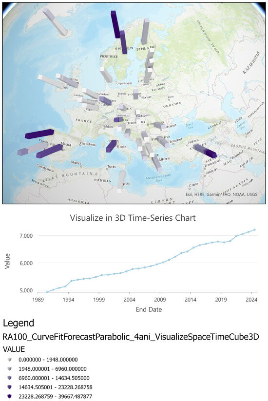
Figure 2.
3D Visualization of the Space-Time Cube for Parabolic Forecast Model for Hydropower Production Capacity, 1990–2025 [74]. Source: authors’ research results.
The overall data trend for MEGAWATTS_N_SUM_ZEROS resulting from the temporal aggregation for all studied locations (European countries) is an annual growth of 8 MW/year, with a probability of p = 0.000.
Figure 3 presents the ESDA 2D visualization of the forecasted values for electricity production capacities from renewable hydropower sources in 2025, estimated using the parabolic forecast model and STC for hydropower capacity production. A polarizing trend is identified. Norway and Turkey raised the bar for the highest performance class to over 26,268 MW in 2025, compared to 23,228 MW in the from STC’s 3D representation of hydropower production capacity. Conversely, the threshold for the lowest performer class in hydropower production capacity is lowered from 1948 MW for the entire period to 915 MW for 2025. At the same time, France, Spain, and Italy show a clustering tendency, covering approximately 1/3 of the surface of Europe, forming a contiguous area with above-average performance classified in the 4th performance class.

Figure 3.
2D Visualization of the Space-Time Cube for Parabolic Forecast Model for Hydropower Production Capacity for 2025 [74]. Source: authors’ research results.
The ArcGIS offers the possibility of extracting from Figure 3 the pop-up representation of the parabolic forecast model for each country, as presented in Figure 4.
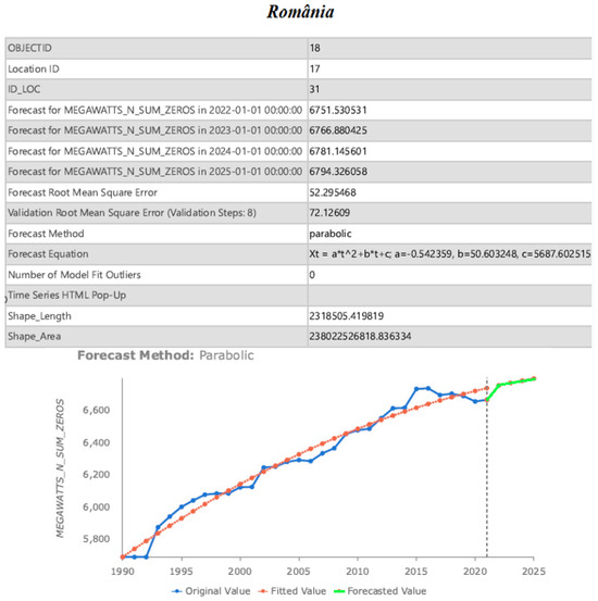
Figure 4.
Quadratic curve fit forecast model for hydropower production capacity in Romania. Source: authors’ research results.
Only the graphic from the Curve fit parabolic forecast representation was retained to comment on the model for all locations.
The curve fit parabolic forecast representation from (a) to (g) has a > 1, and from (h) to (j), 0 < a < 1 (Figure 5). The concave parabolic curve predicts high or less accelerated growth. As the concavity fades, the acceleration of growth in hydropower production capacity also decreases. The representation for Luxemburg shows that in 2013, a radical modification in hydropower production capacity was made, and a new jump could instantly reach a higher level. Disruptions and consistent increases in capacity could result from technological improvements to old producers or the construction of new capacities.
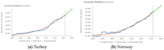
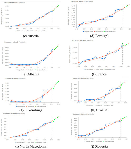
Figure 5.
Positive Quadratic Curve fit forecast model for hydropower production capacity 1990–2025. Source: authors’ research results.
Figure 6 partially presents examples of the convex parabolic forecast results; others will be discussed together with the outliers, since 5 of the 7 outliers are from the negative category.
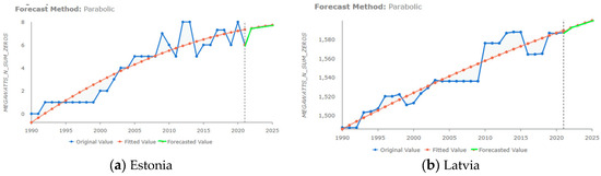
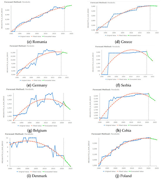
Figure 6.
Negative Quadratic Curve fit forecast model for hydropower production capacity 1990–2025. Source: authors’ research results.
Estonia, Latvia, and Romania have similar trajectories, showing a convex parabolic curve with a slow growth forecast. The model validates the time series for Romania better than for the other two countries. According to the parabolic model, Latvia, Germany, and Greece have a clear convex trajectory with a forecast of decreased capacity. However, for Serbia, the model does not offer a valid result. The time series demonstrates a very high increase from zero to 3000 and then a constant capacity from 1994 to 2021.
4.5. Outliers’ Analysis
The outliers offer an interesting perspective. By applying the Generalized Extreme Studentized Deviate (ESD) test, 7 locations with statistically significant outliers are identified. Only one location is validated as a global outlier with values higher than the adjusted values—Hungary—while the other 6 locations are local outliers with values lower than the adjusted values—Bulgaria, Ireland, Sweden, the United Kingdom, Lithuania, and the Netherlands. Figure 7 presents the hydropower production capacity STC with the outliers.
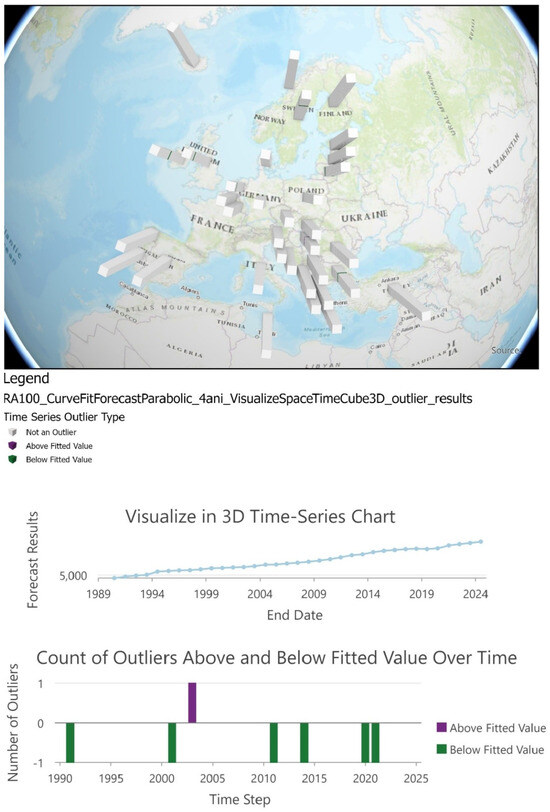
Figure 7.
3D visualization of STC for hydropower production capacity parabolic forecast with outliers [74]. Source: authors’ research results.
The details of the outliers could be analyzed from the Curve fit parabolic forecast representation of each location (see Figure 8).
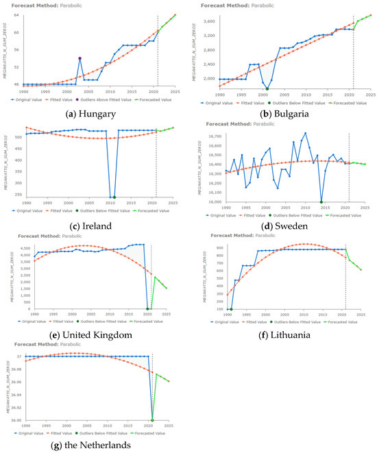
Figure 8.
Quadratic Curve fit forecast model for hydropower production capacity (1990–2025) with outliers. Source: authors’ research results.
Hungary and Ireland belong to the concave parabolic forecast category, although less obviously Ireland. Hungary has a single outlier above the fitted value that cannot be explained, considering that the same value was reached nine years later. Ireland theoretically belongs to the concave curve, but this appears to be due to the outlier values for 2010 and 2011 that corrupted the almost linear trend. That is why the obtained shape was a concave parabola with relative validation. Even if placed on the convex curves, Bulgaria is closer to a linear ascending trend. Similar to Ireland, the United Kingdom, Lithuania, and the Netherlands, the values are mostly linear. However, the outliers placed at the beginning or end generate a convex forecast that is difficult to validate without additional information. Sweden is a completely different case, with constant fluctuations and an outlier for 2015. The existence of production capacity and the high fluctuation in water volume could explain the sawtooth time series in Bulgaria.
4.6. Confidence Level of the Trend
Considering the 2D spatial representation, the confidence trend in hydropower production capacity is presented in Figure 9. The proposed model shows a general uptrend for the period 1990–2025 and a confidence of level 99% for all European countries except for the Netherlands and Denmark (countries with a downtrend and a high confidence level of 99%) and Sweden (confirming the ‘No significant trend identified’ result from the outlier analysis).
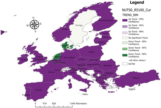
Figure 9.
STC representation of trend direction and confidence level of the Curve fit Parabolic forecast model for Hydropower production capacity in EU countries. Source: authors’ research results.
The output of the Space-Time Pattern Mining Tool is the hydropower production capacity forecast space-time cube visualization in 2D (Figure 9). It allows us to render the netCDF space-time cube in a unique manner in 2D, calculated with a 4-time bin forecast. The netCDF space-time cube is a scientific data format for 3D data. In our case, there were data for each of the 32 time bins in a total of 33 locations for hydropower production capacity for each X and Y coordinate, representing the European countries.
The representation highlighted the already mentioned results of a general uptrend for European countries, this time with a confidence of 95%. The downtrends of the Netherlands and Denmark also have a confidence of 95%.
This reconfirms the high quality of the curve fit parabolic forecast model proposed for predicting the hydropower production capacity in Europe.
5. Discussion
The proposed model is discussed at the European level, considering both the validation of past time series and the forecast, as well as the acceleration regime (double the quadratic coefficient). Considering that “less is better”, VRMSE values were used to validate the parabolic curve fit for the past time series. For 15 of the 33 locations with a VRMSE < 5% of the VRMSEmax, the parabolic model provides a better approximation (Netherlands, Denmark, Estonia, Hungary, Belgium, Croatia, Latvia, Poland, North Macedonia, Italy, Finland, Romania, France, Greece, and Luxembourg).
Moreover, based on the graphical results, the parabolic model offers a better forecast for 14 of the 33 locations (Netherlands, Denmark, Estonia, Hungary, Belgium, Latvia, Croatia, North Macedonia, Finland, Poland, Luxembourg, Romania, Slovenia, and Ireland). The quadratic trajectories fit the raw data for 14 countries, validated by visual inspection, and for 20 countries, validated by an FMRSE threshold of 10% from the maximum value. The quadratic model is suitable for forecasting future values of hydropower production capacity in 22 countries, with accuracy confirmed by the VMRSE with a threshold of 10% from the maximum value. This result confirms that most locations are well approximated and that the proposed forecast model is consistent. The locations that are less well approximated and forecast should be subject to other curve fit models.
Starting from the curve fit forecast parabolic equations generated by the past records of 32 years, the acceleration of the process was determined by analogy with constant acceleration motion. The acceleration (acc) is double the quadratic coefficient. In accordance with kinematic theory, positive acceleration reflects an increase or growth in the velocity variation of electric hydropower production capacity. The higher the value, the more rapid the process. Negative acceleration emphasizes a process of deceleration, reflecting a decrease or reduction in the velocity variation of hydropower production capacity.
Upon the acceleration regime, four location categories were identified:
- (a)
- High positive acceleration (acc > 1): These countries have prospects for intensive expansion, large diversification, and technological modernization of hydro systems. Turkey, Norway, Austria, Portugal, Albania, France, and Luxembourg are countries that specialize in hydropower production and should be considered best practices based on the statistics of the last three decades;
- (b)
- Moderate positive acceleration (0 < acc < 1): This category includes Croatia, North Macedonia, Slovenia, Ireland, Iceland, and Hungary, with prospects for large, extensive expansion, diversification, and technological modernization of hydro systems. Extensive development is also a pathway to consider for the energetic shift to renewable energy;
- (c)
- Low negative acceleration, deceleration (−1 < acc < 0): These countries are characterized by a decrease in hydropower production capacity. The Netherlands, Estonia, Denmark, Latvia, Bulgaria, Belgium, Montenegro, Sweden, and Italy appear to have hydropower infrastructure but have fewer new investments;
- (d)
- High negative acceleration, rapid deceleration (acc < −1): Finland, Romania, Poland, Greece, Spain, Lithuania, Germany, the United Kingdon, Slovakia, and Serbia show constant negative accelerations, practically indicating an accelerated contraction of the hydro sector with prospects of diminishing physical infrastructure and implicitly without investments in new technologies.
Besides the extensive development of hydropower production capacities, which is naturally limited by river availability, digital adoption should be considered to increase and manage production, as well as innovative storage solutions for short- and long-term energy storage from other renewable sources that are less stable than hydropower.
The findings give a perspective on the evolution of the hydropower production capacity of all European countries from 2022 to 2025, and the rate of the model validation confirms the model.
- Hypothesis 1:The curve-fit parabolic forecast model provides a reliable approximation of hydropower production capacities—this was confirmed. The curve fit parabolic forecast model fits 2/3 of the European countries and is a good representation of hydropower production capacities for 1990–2021 in European countries.
- Hypothesis 2: Hydropower production capacities have a general uptrend for the period 1990–2025 in all European countries—yes, the overall data trend for 1990–2021 is an uptrend, with an average annual increase of 8 MW.
- Hypothesis 3: Countries’ capacity to produce electrical hydropower differs by speed and acceleration, and highly accelerated hydropower production capacities are a potential result of digital adoption—yes, there are 13 countries with a positive quadratic tendency of capacity growth, of which 7 present an acceleration over 1. These 7 countries are the countries that apply digital technologies.
- Hypothesis 4: The quadratic model validates the medium-term level forecast of hydropower production capacities for all 33 European countries—no, the validation model indicates accurate forecasts for about 2/3 of the countries, much like those with validated curves that fit the raw data. A long-term perspective regarding hydropower production capacities for these countries is shaped.
- Hypothesis 5: How many outliers does the dataset contain? After applying the Generalized Extreme Studentized Deviate (GESD) test, there were 7 outliers, but after a deep analysis, two outliers were excluded: the United Kingdom and the Netherlands, which have constant hydropower production capacities.
6. Conclusions
The present study addressed the need to provide quantitative evaluations of medium- and short-term predictive estimates, representing valuable input for the adaptive and resilient efficiency of the energy sector, as recommended by the Global Framework for Climate Services [79]. Enhancing adaptability and resilience in the energy sector, which is also crucial for mitigation efforts, requires the development, ongoing improvement, and widespread application of climate services. These services are essential for assessing the potential of wind, solar, and hydroelectric power and making predictive estimates about these energy sources across various forecasting intervals.
Space-time exploration over three decades for almost the entire European area allows us to correlate our results with climate change maps [80]. In the context of climate change, adaptation solutions require using forecasts with long time series that cover large geographical areas and can capture these new patterns.
The green transition requires an integrated approach strongly anchored in strategic frameworks and development construction plans, where the curve fit forecast model’s trajectories provide a long-term perspective. This result is another valuable input for labor force allocation and reallocation to other sectors toward the green sector, a process fueled the appropriate training and formation.
6.1. Theoretical Implication
The proposed curve fit forecast parabolic model for hydropower production capacities contributes to the theory and the literature on energy from renewable sources. It also provides a model to forecast short-term values and medium- and long-term trends. Using space-time representations, the model offers a geographic perspective and the capacity to identify patterns. By enlarging the portfolio of geographic representations, our model contributes to overlapping or multi-layer studies. It has a high potential for replication, either for other regions or regenerative energy sources.
6.2. Managerial Implication
The forecast study aimed to offer scientists and practitioners insights into the trends and perspectives, in our case, for the hydropower sector in Europe as a basis for further developments and socioeconomic implications.
Our study findings about hydropower production capacities in European countries provide decision makers with hints about the perspectives and trends of this regenerative energy source. Each country can decide on the type of development (extensive or intensive) and innovation (incremental or disruptive). The provided information should be correlated with climate change predictions and energy needs.
The patterns and categories identified allow us to analyze best practices and leaders to find already successfully implemented solutions. Moreover, the need for technology and innovation is obvious if it targets disruptive progress. The importance of natural resources and human capital for the integrated framework meant to address today’s challenges should be consistently considered.
6.3. Limits and Further Developments
Among the limitations of our model is the short prediction time of only 4 years, compared to the past time series used (32 years). Another limitation of the model is the validity of the results for a limited number of locations. These generations highlight the need to explore other models that may be more suitable for unvalidated locations. Unfortunately, the model does not offer information about the triggering factors of hydropower production capacities. This limitation can be addressed by overlapping multi-layer models and maps. In our opinion, acceleration seems to be based on technological improvements or digital adoption. The deceleration of production could result from climate change or water flow management.
The study offers multiple research developments, such as exploring other curve fit forecast models for hydropower production capacities, comparing the findings of different models for the studied locations, and applying the models to other types of energy production. It suggests developing an integrated framework for the twin transition (digital and energy) overlaid on climate change or natural resource maps. A topic to be considered for further studies is the water-energy-land-food (WELF) nexus and finding ways to forecast them together.
Author Contributions
Conceptualization, C.L. and A.G.; methodology, C.L. and H.D.; software, C.L.; validation, A.G., C.L. and H.D; formal analysis, A.G. and H.D; investigation, C.L.; resources, C.L.; data curation, C.L. and H.D; writing—original draft preparation, C.L. and A.G.; writing—review and editing, A.G. and H.D; visualization, C.L.; supervision, A.G. and H.D; project administration, A.G.; funding acquisition, A.G. All authors have read and agreed to the published version of the manuscript.
Funding
This research was funded by the Romanian Ministry of Research, Innovation, and Digitalization, Programme NUCLEU, 2022–2026, PN 22_10_0105.
Data Availability Statement
The data used are from public sources mentioned in the main text.
Acknowledgments
This work was supported by a grant from the Romanian Ministry of Research, Innovation, and Digitalization, Programme NUCLEU, 2022–2026, Spatio-temporal forecasting of local labour markets through GIS modelling [P5]/Previziuni spatio-temporale pentru pietele muncii locale prin modelare în GIS [P5] PN 22_10_0105.
Conflicts of Interest
The authors declare no conflicts of interest.
References
- Grigorescu, A.; Ion, A.E.; Lincaru, C.; Pirciog, S. Synergy analysis of knowledge transfer for the energy sector within the framework of sustainable development of the European countries. Energies 2021, 15, 276. [Google Scholar] [CrossRef]
- European Commission. The European Green Deal, COM (2019) 640 Final, EUR-Lex-52019DC0640-EN-EUR-Lex (europa.eu); European Commission: Brussels, Belgium, 2019. [Google Scholar]
- United Nations Framework Convention on Climate Change (UNFCCC). The Paris Agreement, Denmark; parisagreement_publication.pdf (unfccc.int); United Nations: New York, NY, USA, 2016. [Google Scholar]
- European Commission. A Framework Strategy for a Resilient Energy Union with a Forward-Looking Climate Change Policy/* COM/2015/080 final */; EUR-Lex-52015DC0080-EN-EUR-Lex (europa.eu); European Commission: Brussels, Belgium, 2015. [Google Scholar]
- Energy Institute-Statistical Review of World Energy (2023)—With Major Processing by Our World in Data. “Electricity Generation from Hydropower” [Dataset]. Energy Institute, “Statistical Review of World Energy” [Original Data]. Available online: https://ourworldindata.org/grapher/hydro-consumption-by-region (accessed on 27 March 2024).
- Elavarasan, R.M. The motivation for renewable energy and its comparison with other energy sources: A review. Eur. J. Sustain. Dev. Res. 2019, 3, em0076. [Google Scholar] [CrossRef] [PubMed]
- Ristinen, R.A.; Kraushaar, J.J.; Brack, J.T. Energy and the Environment; John Wiley & Sons: Hoboken, NJ, USA, 2022. [Google Scholar]
- Miskat, M.; Ahmed, A.; Rahman, M.S.; Chowdhury, H.; Chowdhury, T.; Chowdhury, P.; Sait, S.M.; Park, Y.K. An overview of the hydropower production potential in Bangladesh to meet the energy requirements. Environ. Eng. Res. 2021, 26, 200514. [Google Scholar] [CrossRef]
- Hdom, H.A.; Fuinhas, J.A. Energy production and trade openness: Assessing economic growth, CO2 emissions and the applicability of the cointegration analysis. Energy Strategy Rev. 2020, 30, 100488. [Google Scholar] [CrossRef]
- Blakers, A.; Stocks, M.; Lu, B.; Cheng, C. A review of pumped hydro energy storage. Prog. Energy 2021, 3, 022003. [Google Scholar] [CrossRef]
- Kuriqi, A.; Pinheiro, A.N.; Sordo-Ward, A.; Garrote, L. Flow regime aspects in determining environmental flows and maximising energy production at run-of-river hydropower plants. Appl. Energy 2019, 256, 113980. [Google Scholar] [CrossRef]
- Guo, Y.; Xu, Y.P.; Xie, J.; Chen, H.; Si, Y.; Liu, J. A weights combined model for middle and long-term streamflow forecasts and its value to hydropower maximization. J. Hydrol. 2021, 602, 126794. [Google Scholar] [CrossRef]
- Kuriqi, A.; Pinheiro, A.N.; Sordo-Ward, A.; Garrote, L. Influence of hydrologically based environmental flow methods on flow alteration and energy production in a run-of-river hydropower plant. J. Clean. Prod. 2019, 232, 1028–1042. [Google Scholar] [CrossRef]
- Kuriqi, A.; Pinheiro, A.N.; Sordo-Ward, A.; Garrote, L. Water-energy-ecosystem nexus: Balancing competing interests at a run-of-river hydropower plant coupling a hydrologic–ecohydraulic approach. Energy Convers. Manag. 2020, 223, 113267. [Google Scholar] [CrossRef]
- Kos, Ž.; Đurin, B.; Dogančić, D.; Kranjčić, N. Hydro-energy suitability of rivers regarding their hydrological and hydrogeological characteristics. Water 2021, 13, 1777. [Google Scholar] [CrossRef]
- Manzano-Agugliaro, F.; Taher, M.; Zapata-Sierra, A.; Juaidi, A.; Montoya, F.G. An overview of research and energy evolution for small hydropower in Europe. Renew. Sustain. Energy Rev. 2017, 75, 476–489. [Google Scholar] [CrossRef]
- Gernaat, D.E.; Bogaart, P.W.; Vuuren, D.P.V.; Biemans, H.; Niessink, R. High-resolution assessment of global technical and economic hydropower potential. Nat. Energy 2017, 2, 821–828. [Google Scholar] [CrossRef]
- Hoes, O.A.; Meijer, L.J.; Van Der Ent, R.J.; Van De Giesen, N.C. Systematic high-resolution assessment of global hydropower potential. PLoS ONE 2017, 12, e0171844. [Google Scholar] [CrossRef] [PubMed]
- Hunt, J.D.; Byers, E.; Wada, Y.; Parkinson, S.; Gernaat, D.E.; Langan, S.; van Vuuren, D.P.; Riahi, K. Global resource potential of seasonal pumped hydropower storage for energy and water storage. Nat. Commun. 2020, 11, 947. [Google Scholar] [CrossRef] [PubMed]
- Moran, E.F.; Lopez, M.C.; Moore, N.; Müller, N.; Hyndman, D.W. Sustainable hydropower in the 21st century. Proc. Natl. Acad. Sci. USA 2018, 115, 11891–11898. [Google Scholar] [CrossRef] [PubMed]
- Popa, F.; Dumitran, G.E.; Vuta, L.I.; Tica, E.I.; Popa, B.; Neagoe, A. Impact of the ecological flow of some small hydropower plants on their energy production in Romania. J. Phys. Conf. Ser. 2020, 1426, 012043. [Google Scholar] [CrossRef]
- Tiruye, G.A.; Besha, A.T.; Mekonnen, Y.S.; Benti, N.E.; Gebreslase, G.A.; Tufa, R.A. Opportunities and challenges of renewable energy production in Ethiopia. Sustainability 2021, 13, 10381. [Google Scholar] [CrossRef]
- Lehner, B.; Liermann, C.R.; Revenga, C.; Vörösmarty, C.; Fekete, B.; Crouzet, P.; Döll, P.; Endejan, M.; Frenken, K.; Magome, J.; et al. Highresolution mapping of the world’s reservoirs and dams for sustainable river-flow management. Front. Ecol. Environ. 2011, 9, 494–502. [Google Scholar] [CrossRef] [PubMed]
- Zarfl, C.; Lumsdon, A.E.; Berlekamp, J.; Tydecks, L.; Tockner, K. A global boom in hydropower dam construction. Aquat. Sci. 2015, 77, 161–170. [Google Scholar] [CrossRef]
- Ahmad, S.K.; Hossain, F. Forecast-informed hydropower optimization at long and short-time scales for a multiple dam network. J. Renew. Sustain. Energy 2020, 12, 014501. [Google Scholar] [CrossRef]
- Hirth, L. The benefits of flexibility: The value of wind energy with hydropower. Appl. Energy 2016, 181, 210–223. [Google Scholar] [CrossRef]
- Malhan, P.; Mittal, M. A novel ensemble model for long-term forecasting of wind and hydro power generation. Energy Convers. Manag. 2022, 251, 114983. [Google Scholar] [CrossRef]
- Kougias, I.; Szabo, S.; Monforti-Ferrario, F.; Huld, T.; Bódis, K. A methodology for optimization of the complementarity between small-hydropower plants and solar PV systems. Renew. Energy 2016, 87, 1023–1030. [Google Scholar] [CrossRef]
- Kougias, I.; Aggidis, G.; Avellan, F.; Deniz, S.; Lundin, U.; Moro, A.; Muntean, S.; Novara, D.; Pérez-Díaz, J.I.; Quaranta, E.; et al. Analysis of emerging technologies in the hydropower sector. Renew. Sustain. Energy Rev. 2019, 113, 109257. [Google Scholar] [CrossRef]
- Yuksel, I.; Arman, H.; Serencam, U. Hydro energy and environmental policies in Turkey. J. Therm. Eng. 2016, 2, 934–939. [Google Scholar]
- Ahmad, S.K.; Hossain, F. Maximizing energy production from hydropower dams using short-term weather forecasts. Renew. Energy 2020, 146, 1560–1577. [Google Scholar] [CrossRef]
- Yah, N.F.; Oumer, A.N.; Idris, M.S. Small scale hydro-power as a source of renewable energy in Malaysia: A review. Renew. Sustain. Energy Rev. 2017, 72, 228–239. [Google Scholar] [CrossRef]
- Kuriqi, A.; Pinheiro, A.N.; Sordo-Ward, A.; Bejarano, M.D.; Garrote, L. Ecological impacts of run-of-river hydropower plants—Current status and future prospects on the brink of energy transition. Renew. Sustain. Energy Rev. 2021, 142, 110833. [Google Scholar] [CrossRef]
- Barbosa, L.D.S.N.S.; Bogdanov, D.; Vainikka, P.; Breyer, C. Hydro, wind and solar power as a base for a 100% renewable energy supply for South and Central America. PLoS ONE 2017, 12, e0173820. [Google Scholar] [CrossRef] [PubMed]
- Spiru, P. Assessment of renewable energy generated by a hybrid system based on wind, hydro, solar, and biomass sources for decarbonizing the energy sector and achieving a sustainable energy transition. Energy Rep. 2023, 9, 167–174. [Google Scholar] [CrossRef]
- Stadelmann-Steffen, I.; Rieder, S.; Strotz, C. The politics of renewable energy production in a federal context: The deployment of small hydropower in the Swiss cantons. J. Environ. Dev. 2020, 29, 75–98. [Google Scholar] [CrossRef]
- Baloch, Z.A.; Tan, Q.; Kamran, H.W.; Nawaz, M.A.; Albashar, G.; Hameed, J. A multi-perspective assessment approach of renewable energy production: Policy perspective analysis. Environ. Dev. Sustain. 2021, 24, 2164–2192. [Google Scholar] [CrossRef]
- Zafar, U.; Ur Rashid, T.; Khosa, A.A.; Khalil, M.S.; Rashid, M. An overview of implemented renewable energy policy of Pakistan. Renew. Sustain. Energy Rev. 2018, 82, 654–665. [Google Scholar] [CrossRef]
- Drakaki, K.K.; Sakki, G.K.; Tsoukalas, I.; Kossieris, P.; Efstratiadis, A. Day-ahead energy production in small hydropower plants: Uncertainty-aware forecasts through effective coupling of knowledge and data. Adv. Geosci. 2022, 56, 155–162. [Google Scholar] [CrossRef]
- Bordin, C.; Skjelbred, H.I.; Kong, J.; Yang, Z. Machine learning for hydropower scheduling: State of the art and future research directions. Procedia Comput. Sci. 2020, 176, 1659–1668. [Google Scholar] [CrossRef]
- Jurasz, J.; Kies, A.; Zajac, P. Synergetic operation of photovoltaic and hydro power stations on a day-ahead energy market. Energy 2020, 212, 118686. [Google Scholar] [CrossRef]
- Hatata, A.Y.; El-Saadawi, M.M.; Saad, S. A feasibility study of small hydro power for selected locations in Egypt. Energy Strategy Rev. 2019, 24, 300–313. [Google Scholar] [CrossRef]
- Azad, A.S.; Rahaman, M.S.A.; Watada, J.; Vasant, P.; Vintaned, J.A.G. Optimization of the hydropower energy generation using Meta-Heuristic approaches: A review. Energy Rep. 2020, 6, 2230–2248. [Google Scholar] [CrossRef]
- Zhou, F.; Li, L.; Zhang, K.; Trajcevski, G.; Yao, F.; Huang, Y.; Zhong, T.; Wang, J.; Liu, Q. Forecasting the evolution of hydropower generation. In Proceedings of the 26th ACM SIGKDD International Conference on Knowledge Discovery & Data Mining, Virtual, 6–10 July 2020; pp. 2861–2870. [Google Scholar]
- Rahman, M.M.; Shakeri, M.; Tiong, S.K.; Khatun, F.; Amin, N.; Pasupuleti, J.; Hasan, M.K. Prospective methodologies in hybrid renewable energy systems for energy prediction using artificial neural networks. Sustainability 2021, 13, 2393. [Google Scholar] [CrossRef]
- Parvez, I.; Shen, J.; Hassan, I.; Zhang, N. Generation of hydro energy by using data mining algorithm for cascaded hydropower plant. Energies 2021, 14, 298. [Google Scholar] [CrossRef]
- Ding, Z.; Wen, X.; Tan, Q.; Yang, T.; Fang, G.; Lei, X.; Zhang, Y.; Wang, H. A forecast-driven decision-making model for long-term operation of a hydro-wind-photovoltaic hybrid system. Appl. Energy 2021, 291, 116820. [Google Scholar] [CrossRef]
- Hammid, A.T.; Sulaiman, M.H.B.; Abdalla, A.N. Prediction of small hydropower plant power production in Himreen Lake dam (HLD) using artificial neural network. Alex. Eng. J. 2018, 57, 211–221. [Google Scholar] [CrossRef]
- Ichiyanagi, K.; Kobayashi, H.; Matsumura, T.; Kito, Y. Application of artificial neural network to forecasting methods of time variation of the flow rate into a dam for a hydro-power plant. In Proceedings of the Second International Forum on Applications of Neural Networks to Power Systems, Yokohama, Japan, 19–22 April 1992; pp. 349–354. [Google Scholar]
- Stokelj, T.; Golob, R. Application of neural networks for hydro power plant water inflow forecasting. In Proceedings of the 5th Seminar on Neural Network Applications in Electrical Engineering, Belgrade, Yugoslavia, 27 September 2000; pp. 189–193. [Google Scholar]
- Cobaner, M.; Haktanir, T.; Kisi, O. Prediction of hydropower energy using ANN for the feasibility of hydropower plant installation to an existing irrigation dam. Water Resour. Manag. 2008, 22, 757–774. [Google Scholar] [CrossRef]
- Lopes, M.N.G.; da Rocha, B.R.P.; Vieira, A.C.; de Sá, J.A.S.; Rolim, P.A.M.; da Silva, A.G. Artificial neural networks approaches for predicting the potential for hydropower generation: A case study for Amazon region. J. Intell. Fuzzy Syst. 2019, 36, 5757–5772. [Google Scholar] [CrossRef]
- Guo, L.N.; She, C.; Kong, D.B.; Yan, S.L.; Xu, Y.P.; Khayatnezhad, M.; Gholinia, F. Prediction of the effects of climate change on hydroelectric generation, electricity demand, and emissions of greenhouse gases under climatic scenarios and optimized ANN model. Energy Rep. 2021, 7, 5431–5445. [Google Scholar] [CrossRef]
- Bernardes Jr, J.; Santos, M.; Abreu, T.; Prado Jr, L.; Miranda, D.; Julio, R.; Viana, P.; Fonseca, M.; Bortoni, E.; Bastos, G.S. Hydropower operation optimization using machine learning: A systematic review. AI 2022, 3, 78–99. [Google Scholar] [CrossRef]
- Avesani, D.; Zanfei, A.; Di Marco, N.; Galletti, A.; Ravazzolo, F.; Righetti, M.; Majone, B. Short-term hydropower optimization driven by innovative time-adapting econometric model. Appl. Energy 2022, 310, 118510. [Google Scholar] [CrossRef]
- Condemi, C.; Casillas-Perez, D.; Mastroeni, L.; Jiménez-Fernández, S.; Salcedo-Sanz, S. Hydro-power production capacity prediction based on machine learning regression techniques. Knowl.-Based Syst. 2021, 222, 107012. [Google Scholar] [CrossRef]
- Sapitang, M.M.; Ridwan, W.; Faizal Kushiar, K.; Najah Ahmed, A.; El-Shafie, A. Machine learning application in reservoir water level forecasting for sustainable hydropower generation strategy. Sustainability 2020, 12, 6121. [Google Scholar] [CrossRef]
- Sweeney, C.; Bessa, R.J.; Browell, J.; Pinson, P. The future of forecasting for renewable energy. Wiley Interdiscip. Rev. Energy Environ. 2020, 9, e365. [Google Scholar] [CrossRef]
- Brodny, J.; Tutak, M.; Saki, S.A. Forecasting the structure of energy production from renewable energy sources and biofuels in Poland. Energies 2020, 13, 2539. [Google Scholar] [CrossRef]
- Stefenon, S.F.; Ribeiro, M.H.D.M.; Nied, A.; Yow, K.C.; Mariani, V.C.; dos Santos Coelho, L.; Seman, L.O. Time series forecasting using ensemble learning methods for emergency prevention in hydroelectric power plants with dam. Electr. Power Syst. Res. 2022, 202, 107584. [Google Scholar] [CrossRef]
- Jamil, R. Hydroelectricity consumption forecast for Pakistan using ARIMA modeling and supply-demand analysis for the year 2030. Renew. Energy 2020, 154, 1–10. [Google Scholar] [CrossRef]
- Şahin, U. Projections of Turkey’s electricity generation and installed capacity from total renewable and hydro energy using fractional nonlinear grey Bernoulli model and its reduced forms. Sustain. Prod. Consum. 2020, 23, 52–62. [Google Scholar] [CrossRef]
- Pata, U.K.; Aydin, M. Testing the EKC hypothesis for the top six hydropower energy-consuming countries: Evidence from Fourier Bootstrap ARDL procedure. J. Clean. Prod. 2020, 264, 121699. [Google Scholar] [CrossRef]
- Chen, C.; Liu, H.; Xiao, Y.; Zhu, F.; Ding, L.; Yang, F. Power Generation Scheduling for a Hydro-Wind-Solar Hybrid System: A Systematic Survey and Prospect. Energies 2022, 15, 8747. [Google Scholar] [CrossRef]
- Zhang, Y.; Cheng, C.; Cao, R.; Li, G.; Shen, J.; Wu, X. Multivariate probabilistic forecasting and its performance’s impacts on long-term dispatch of hydro-wind hybrid systems. Appl. Energy 2021, 283, 116243. [Google Scholar] [CrossRef]
- Tan, Q.; Wen, X.; Sun, Y.; Lei, X.; Wang, Z.; Qin, G. Evaluation of the risk and benefit of the complementary operation of the large wind-photovoltaic-hydropower system considering forecast uncertainty. Appl. Energy 2021, 285, 116442. [Google Scholar] [CrossRef]
- Klosterman, R.E.; Brooks, K.; Drucker, J.; Feser, E.; Renski, H. Planning Support Methods: Urban and Regional Analysis and Projection; Rowman & Littlefield: Lanham, MD, USA, 2018. [Google Scholar]
- Buie, L. Introducing Time Series Forecasting in ArcGIS Pro. ArcGIS Blog. Available online: https://www.esri.com/arcgis-blog/products/arcgis-pro/announcements/introducing-time-series-forecasting-in-arcgis-pro/ (accessed on 28 July 2020).
- ESRI. How Forest-Based Forecast Works. ArcGIS Pro. Available online: https://pro.arcgis.com/en/pro-app/latest/tool-reference/space-time-pattern-mining/learnmoreforestbasedforecast.htm (accessed on 7 November 2023).
- Seradayan, L.; Mosinyan, A.; Kotolyan, A. Difference between Prediction and Forecast. platAI. Available online: https://plat.ai/blog/difference-between-prediction-and-forecast/ (accessed on 26 June 2023).
- Bakshi, A. What’s New for Spatial Statistics in ArcGIS Pro 2.7? ArcGis Blog. Available online: https://www.esri.com/arcgis-blog/products/arcgis-pro/analytics/whats-new-for-spatial-statistics-in-arcgis-pro-2-7/ (accessed on 23 December 2020).
- Chai, T.; Draxler, R.R. Root mean square error (RMSE) or mean absolute error (MAE)?–Arguments against avoiding RMSE in the literature. Geosci. Model Dev. 2014, 7, 1247–1250. [Google Scholar] [CrossRef]
- Hodson, T.O. Root-mean-square error (RMSE) or mean absolute error (MAE): When to use them or not, Geosci. Model Dev. 2022, 15, 5481–5487. [Google Scholar] [CrossRef]
- ESRI. Arc Gis PRo 3.1, Understanding Outliers in Time Series Analysis ArcGIS Pro 3.1. 2023. Available online: https://pro.arcgis.com/en/pro-app/3.1/tool-reference/space-time-pattern-mining/understanding-outliers-in-time-series-analysis.htm#:~:text=Outliers%20in%20time%20series%20data,outliers%20in%20their%20time%20series (accessed on 1 June 2023).
- Grubbs, F. Procedures for Detecting Outlying Observations in Samples. Technometrics 1969, 11, 1–21. [Google Scholar] [CrossRef]
- Stefansky, W. Rejecting Outliers in Factorial Designs. Technometrics 1972, 14, 469–479. [Google Scholar] [CrossRef]
- Kendall, M.G.; Gibbons, J.D. Rank Correlation Methods, fifth ed.; Griffin: London, UK, 1990. [Google Scholar]
- Eurostat Database. Available online: https://ec.europa.eu/eurostat/databrowser//product/view/NRG_INF_EPCRW (accessed on 5 June 2023).
- GFCS. Energy. Global Framework for Climate Services (GFCS). Global Framework for Climate Services (GFCS). 2017. Available online: https://wmo.int/site/global-framework-climate-services-gfcs (accessed on 2 October 2023).
- Bojariu, R.; Chiţu, Z.; Dascălu, S.I.; Gothard, M.; Velea, L.F.; Burcea, R.; Dumitrescu, A.; Burcea, S.; Apostol, L.; Amihaesei, V.; et al. Schimbările Climatice—De la Bazele Fizice la Riscuri și Adaptare, II a. ed.; Printech: Mangaluru, India, 2021. [Google Scholar]
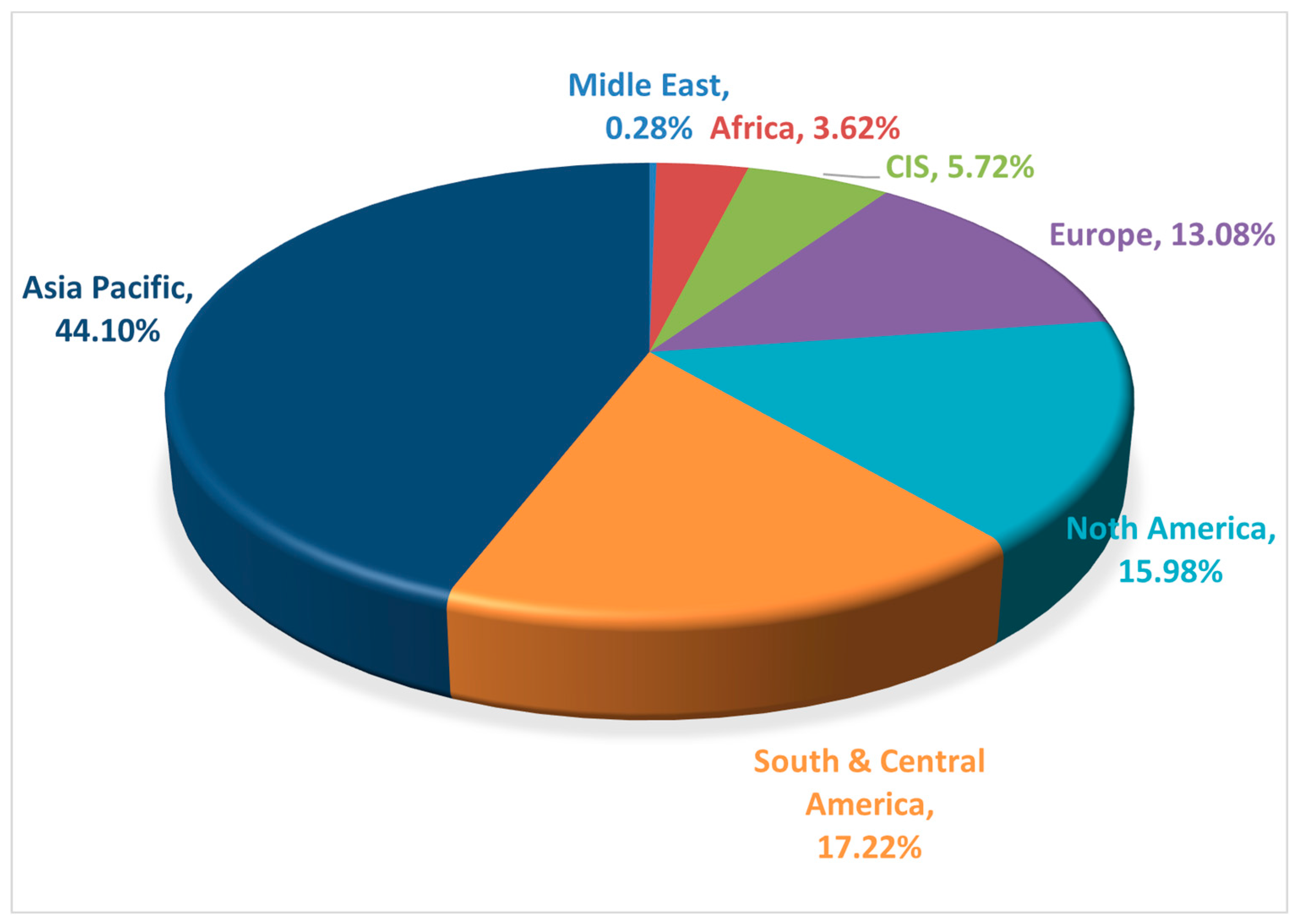

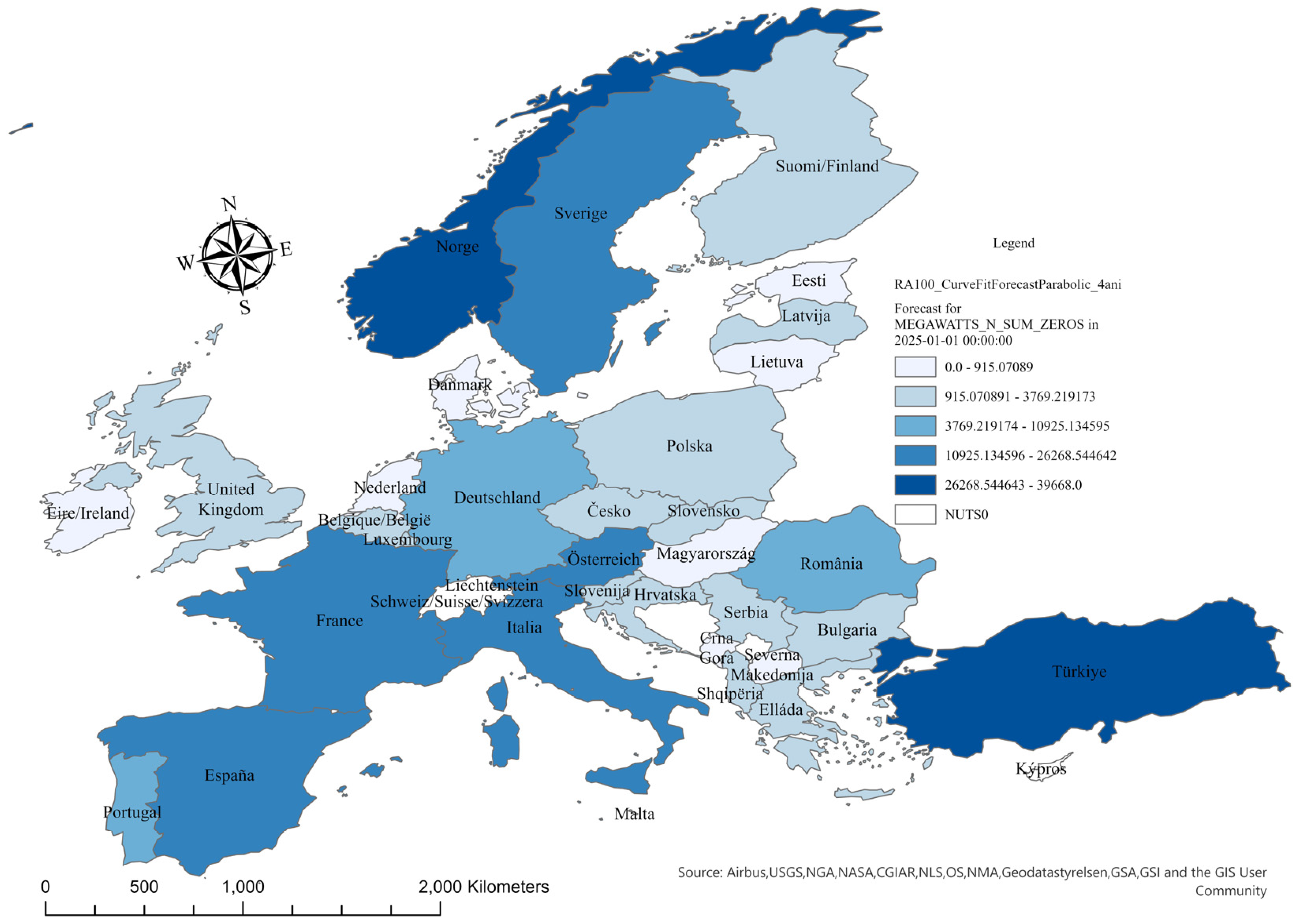
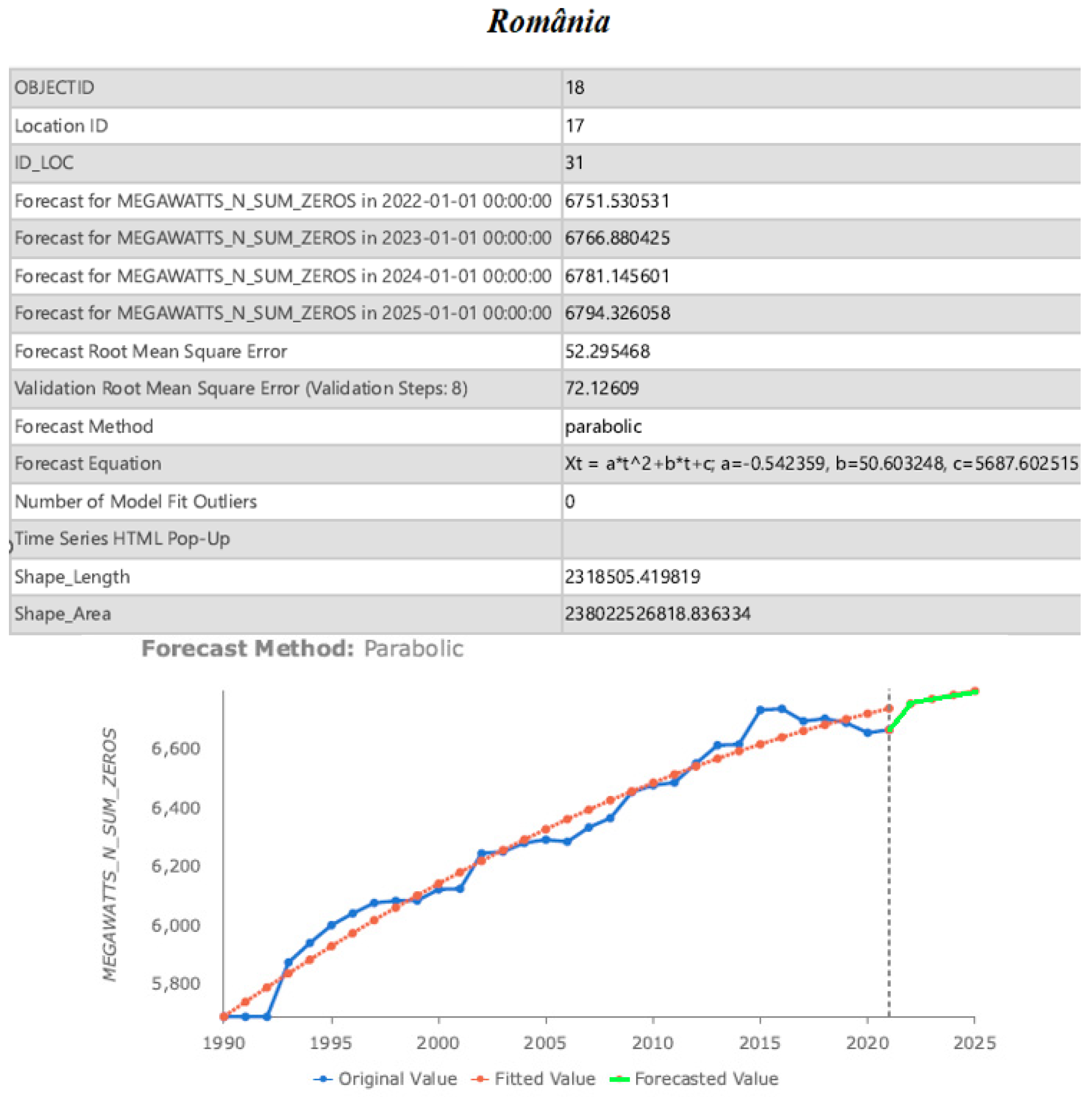
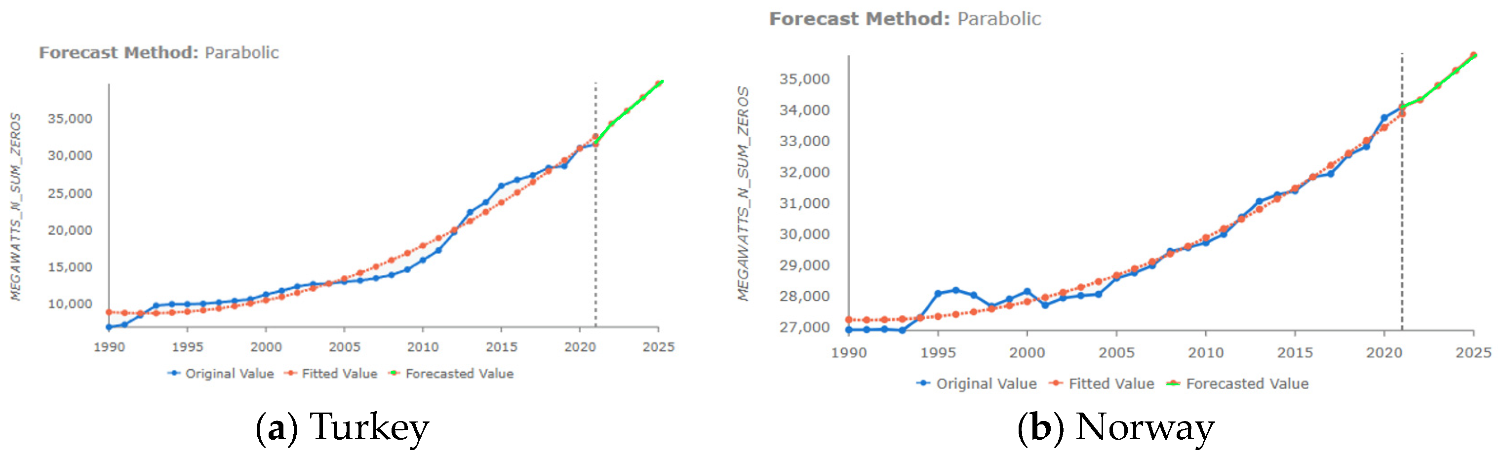
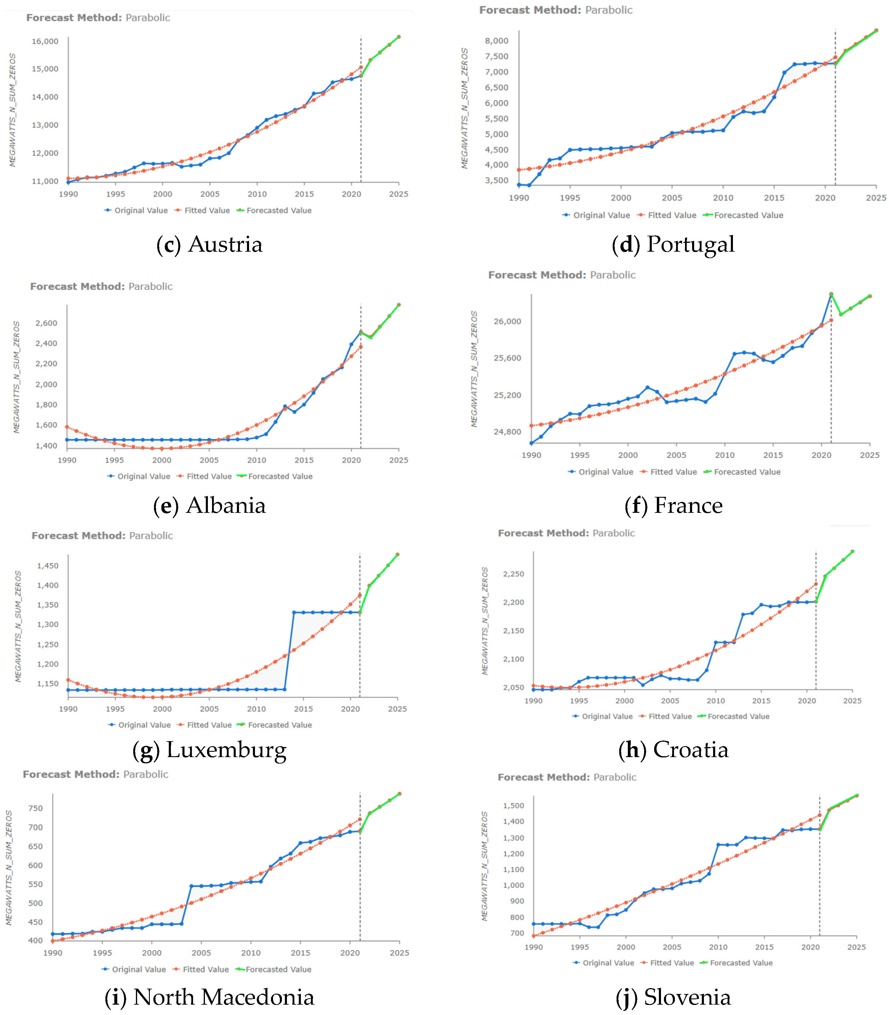
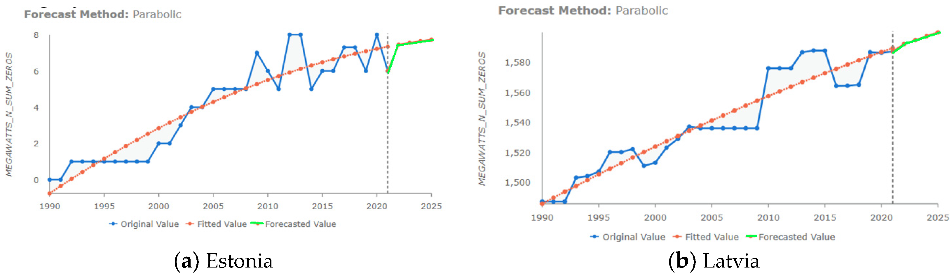
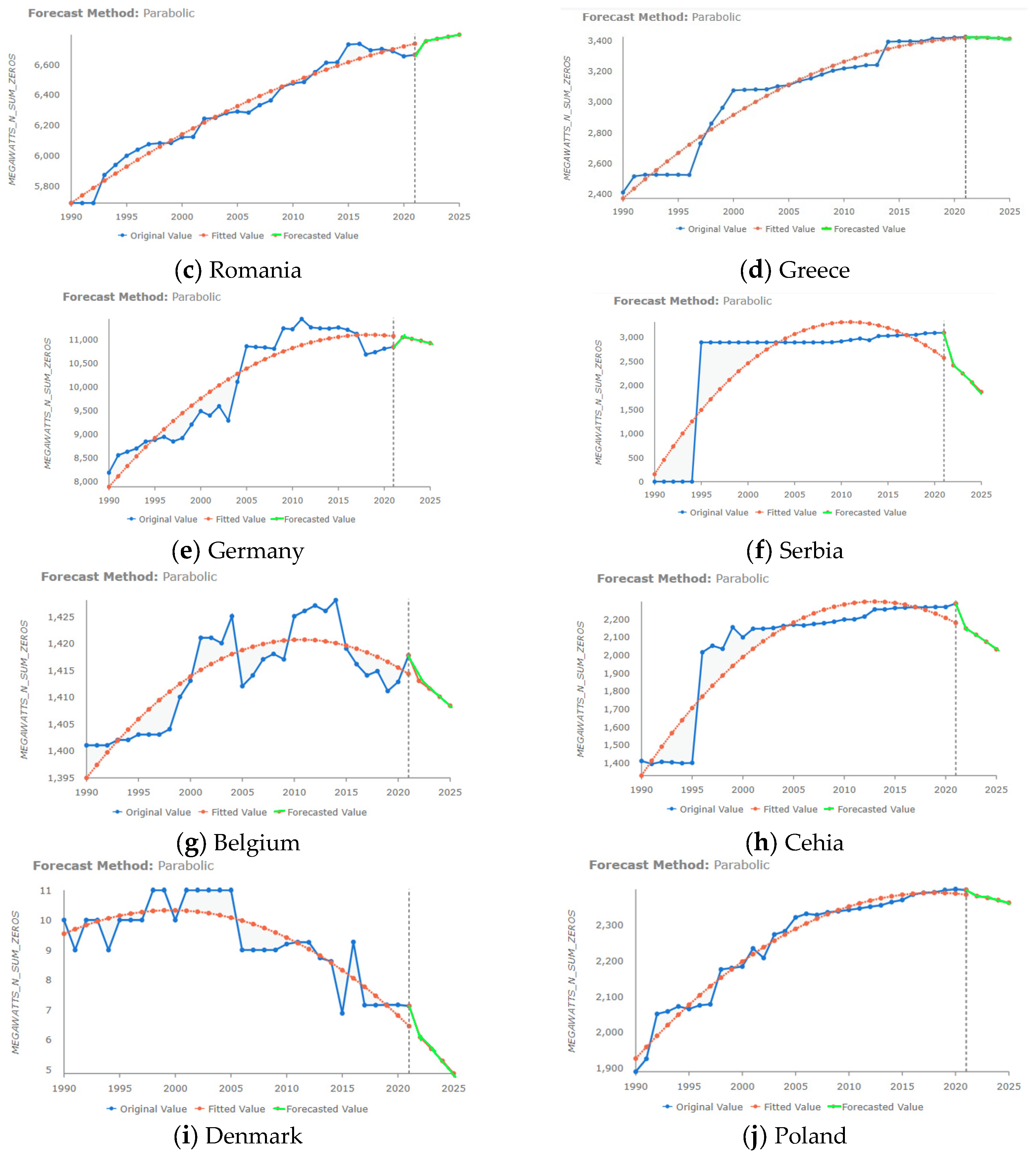

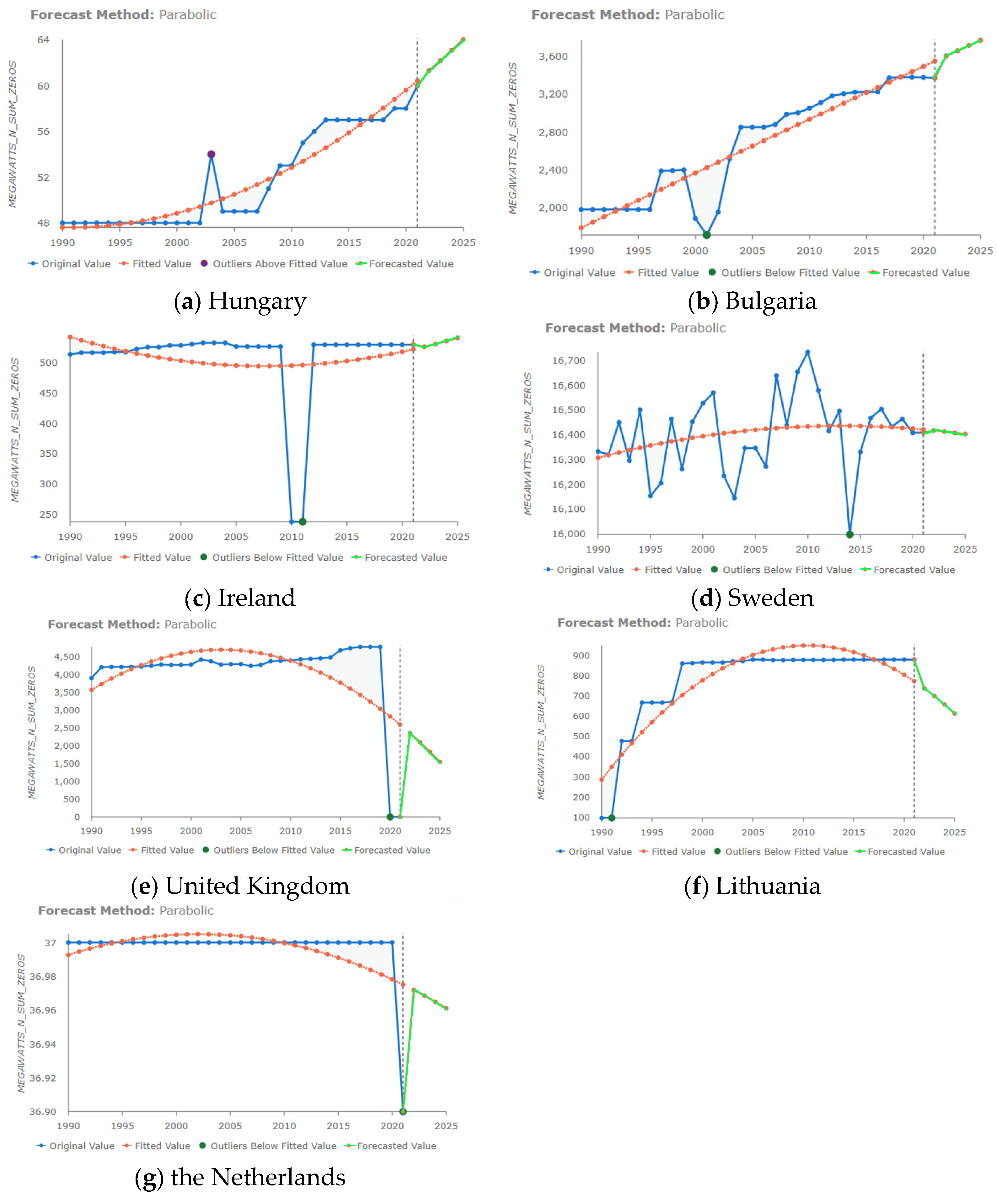

Disclaimer/Publisher’s Note: The statements, opinions and data contained in all publications are solely those of the individual author(s) and contributor(s) and not of MDPI and/or the editor(s). MDPI and/or the editor(s) disclaim responsibility for any injury to people or property resulting from any ideas, methods, instructions or products referred to in the content. |
© 2024 by the authors. Licensee MDPI, Basel, Switzerland. This article is an open access article distributed under the terms and conditions of the Creative Commons Attribution (CC BY) license (https://creativecommons.org/licenses/by/4.0/).