Three-Dimensional Heterogeneous Salt Cavern Underground Gas Storage Water Solution Cavity Model Study

Abstract

In recent years, with the rapid development of salt cavern gas storage reservoir construction in China, the characteristics of salt rock reservoirs with strong non-homogeneity and many interlayers have brought challenges to the dynamic prediction of water solution cavity construction. Aiming to solve this problem, this paper constructs a three-dimensional non-homogeneous salt cavern reservoir water-soluble cavity building prediction model, which takes into full consideration the non-homogeneity of salt rock reservoirs, interlayers, reservoir temperatures, and water injection process parameters, among other factors. By comparing the calculation results of the software compiled by the model with those of other numerical simulation software, we show that the model can accurately reflect the influence of geological parameters on the cavity morphology under the condition of non-uniform geological parameters, with higher simulation accuracy, and ultimately analyze individual examples. It can provide important theoretical support and practical guidance for the construction of a salt cavern gas storage reservoir.

1. Introduction

Salt cavern gas storage has gained significant attention in China due to its advantages of large storage capacity, high safety, and low construction costs, making it a critical component in the field of natural gas reserves [1,2,3,4,5]. The structural properties of salt rock enable it to be utilized not only for storing hydrocarbons but also for the containment of waste in backfill mixtures, demonstrating its versatile application potential.

The construction of salt cavern gas storage facilities necessitates precise prediction of the water solution cavity morphology and volume, thus making the modeling of salt rock water solution cavities a key area of current research. Accurate modeling is essential for ensuring the efficiency and safety of these storage systems.

Historically, several significant advancements have been made in this field. In 1974, Nolen J.S. et al. [6] established a pioneering mathematical model of water solution cavity formation in a column coordinate system and developed the CAVSIM3D2.0 software, which laid the foundation for subsequent research. In 1986, Reda D.C. et al. [7] conducted comprehensive laboratory experiments on sealed and pressurized water solution cavity formation in salt rock specimens, simulating the entire process of cavity development. By 1990, KUNKOP of CHEMKOP, Poland, developed new simulation software for water solution cavity formation in salt rocks. In the same year, Kunstman A.S. et al. [8] released the UbroNET software, significantly advancing the field with new capabilities. In 2005, Banfansheng et al. [9] proposed an innovative mathematical model for water solution cavity formation based on Fick’s law of diffusion, Navier–Stokes equations, and convective diffusion equations, introducing a more comprehensive approach to the modeling process. In 2012, Norbert Grüschow et al. [10] incorporated NaCl dissolution and mass cycling effects into their numerical model, integrating Navier–Stokes equations, heat transfer, and turbulent mass transfer equations to better simulate water solution cavity formation. Between 2016 and 2019, Jinlong Li et al. [11,12,13] developed a sophisticated model for cavity expansion that considered insoluble accumulation and the natural gas blocking solvent remediation process, leading to the development of the cavern leaching simulation (CLS3.0) software. In 2021, Katarzyna Cy et al. [14] introduced further refinements to these models, enhancing the accuracy of cavity morphology predictions under various operational conditions.

Recently, Cyran and Kowalski [15] evaluated the stability of different salt cavern shapes under various geological conditions, providing valuable insights for optimizing cavern design for energy storage. Li et al. (2022) [16] proposed a machine-learning-based method for the rapid capacity prediction and construction parameter optimization of energy storage salt caverns, significantly improving prediction efficiency and meeting engineering design requirements. Additionally, a study by Wang et al. (2024) [17] introduced a creep model to analyze the stability of horizontal salt caverns used for different types of energy storage under varying geological conditions, offering practical guidelines for optimizing construction and operation.

Despite these advancements, challenges remain in accurately predicting the behavior of heterogeneous salt formations under varying geological and operational conditions. Our study aims to address these shortcomings by developing a three-dimensional heterogeneous salt cavern model that incorporates current advances in water solution cavity building in salt cavern reservoirs. This model will provide more accurate predictions of cavity morphology and stability, thereby enhancing the safety and efficiency of salt cavern gas storage operations time.

2. Materials and Methods

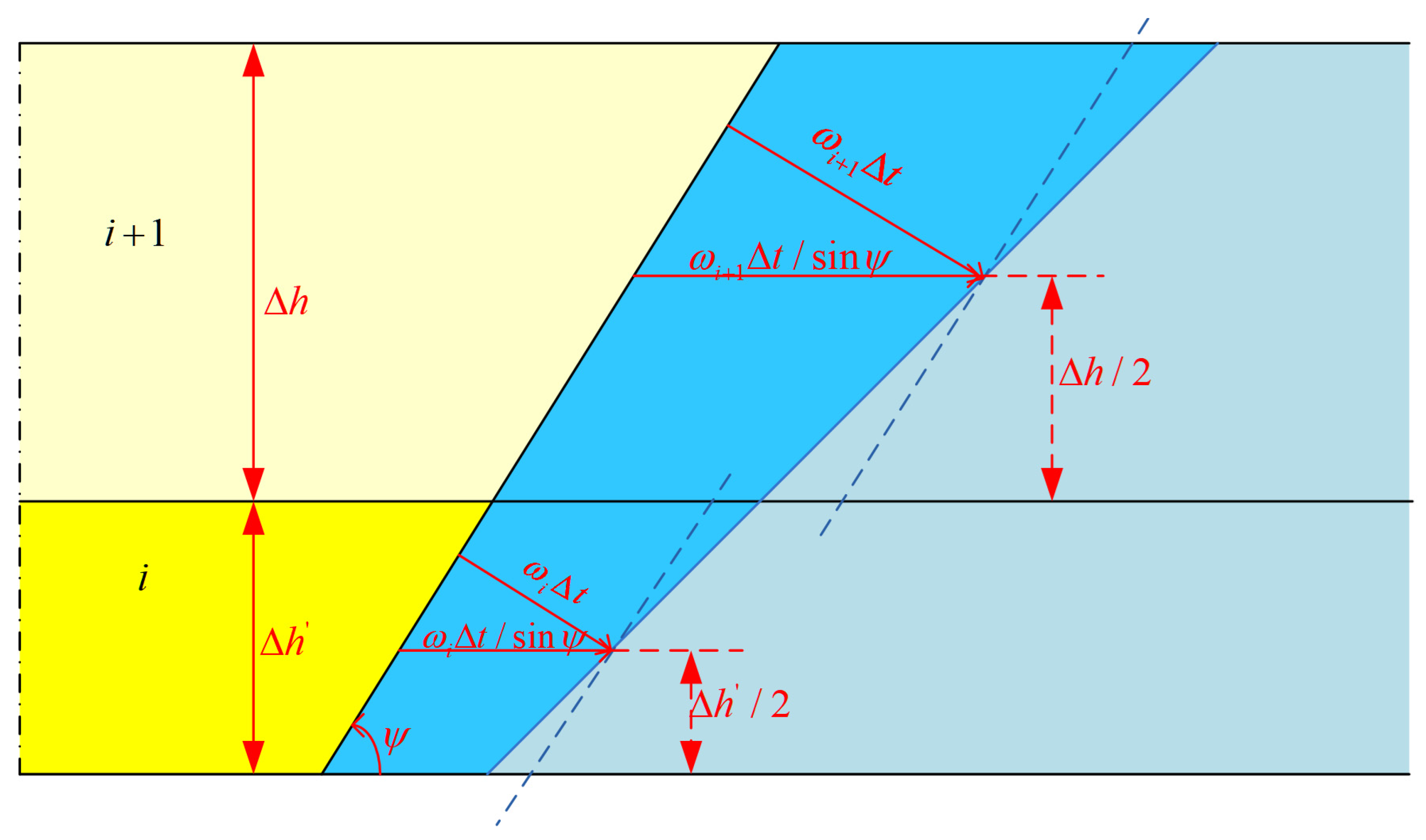
2.1. Mathematical Modelling of Cavity Expansion

Currently, most of the mathematical models for water solution cavity building in salt rock reservoirs [18,19,20] adopt the equivalent cut-point method introduced by Sabrian [21] to describe the cavity profile, as shown in Figure 1a. This method splits the salt rock reservoir into a series of fixed-height slices and solves for the radii of the corresponding height slices at different time steps during the cavity expansion process, thus deriving the cavity profile at the next time step. This method is convenient, simple, and fast to calculate, but there is a big defect: since the height of each point is fixed, the tangent point displacement only occurs in the horizontal direction, the salt rock at the top cannot rise, and the tilt angle of the salt rock at the side cannot be correctly reflected; it is easy to increase the radius of the slices where they are located at certain points and, in turn, to reduce the radius of the slices below so that the originally flat sidewalls become jagged, as shown in Figure 1b [22].

In order to avoid the jagged-like cavity, this paper adopts the equivalent line segment method to describe the cavity contour, as shown in Figure 2. The actual contour of the cavity is the red curve in the figure, which is approximated as a number of blue line segments; each line segment is determined by the starting point (H_i, R_i) and the end point (H_i+1, R_i+1). This method requires high measurement accuracy, and in order to further improve the accuracy of the model, measurement errors also need to be considered. Measurement errors mainly come from the precision limitations of experimental equipment and human operation errors. In the calculation process, these errors may lead to deviations between the actual measured values and the theoretical values. In order to minimize this effect, the effect of random errors can be reduced by taking the average value of multiple measurements. In addition, the experiment should try to ensure the calibration of the measurement equipment and the operation specification to reduce the systematic error.

The equation of the line corresponding to each equivalent line segment can be expressed by the following equation:

$$r=a_{i}h+b_i,$$

(1)

where h is the depth of a point of the line, m; r is the radius of a point of the line; and i denotes the slice number.

$$a_i=\frac{R_{i+1}-R_i}{H_{i+1}-H_i},$$

(2)

$$b_i=R_i-a_i{H}_i=\frac{R_i{H}_{i+1}-R_{i+1}{H}_i}{H_{i+1}-H_i},$$

(3)

where H_i is the contour point depth, m; and R_i is the radius of the contour point, m.

The contour point depth must satisfy the monotonic condition:

$$H_{i }>H_{i+1}.$$

The increment of displacement and the radius of the cavity profile in the direction normal to the profile is expressed by the following equation (the increment is shown schematically in Figure 3):

$$\mathsf{\Delta }n(h)=\omega (h)\mathsf{\Delta }t,$$

(4)

$$\mathsf{\Delta }r(h)=\frac{\omega (h)\mathsf{\Delta }t}{\sin \psi },$$

(5)

where $\Delta n$ is the normal vector increment, m; $\Delta r$ is the radius increment, m; t is the time step, s; Ψ is the inclination angle of the salt rock wall; and $\omega$ is the dissolution rate, m/s, which is determined by the empirical formula for the dissolution rate [23]:

$$\omega =\{\begin{array}{c}{\omega }_d\left(1-C/C_N\right)(1-P_N){(\sin \psi )}^{0.25}\ln \frac{T^{0.44}}{e}(0<\psi \le \pi /2)\hfill \\ {\omega }_d\left(1-C/C_N\right)(1-P_N)\frac{180-\psi }{90}\ln \frac{T^{0.44}}{e}(\pi /2<\psi \le \pi )\hfill \end{array},$$

(6)

where ω_d is the lateral dissolution rate (measured in the laboratory), m/s; C_N is the saturated brine concentration, kg/m³; C is the control body brine concentration, kg/m³; P_N is the insoluble content; and T is the temperature, °C.

a_i has the following geometric relationship with ψ_i:

$$a_i=-ctg{\psi }_i,$$

(7)

$$\sin {\psi }_i=\frac{1}{\sqrt{a_i^2+1}}.$$

(8)

For the case where a line segment contains only one layer of slices, we solve for the a′ and b′ values of the line segment where the next time step of the cavity is located according to Equations (4)–(8):

$$r=a_i^{\prime }h+b_i^{\prime },$$

(9)

$$a_i^{\prime }=a_i,$$

(10)

$$b_i^{\prime }=b_i+\mathsf{\Delta }{R}_i=b_i+\frac{\omega \left(H_i\right)\mathsf{\Delta }t}{\sin {\psi }_i}=b_i+\omega \left(H_i\right)\mathsf{\Delta }t\sqrt{1+a_i^2}.$$

(11)

If a line passes through two slices, then the following applies:

$$a_i^{\prime }=a_i+\frac{\left({\omega }_{i+1}-{\omega }_i\right)\Delta t\sqrt{1+a_i^2}}{H_{i+1}-H_i},$$

(12)

$$b_i^{\prime }=b_i+\frac{\left({\omega }_i{H}_{i+1}-{\omega }_{i+1}{H}_i\right)\mathsf{\Delta }t\sqrt{1+a_i^2}}{H_{i+1}-H_i}.$$

(13)

The more general case, i.e., cases containing multiple concentration slices, using the least squares method, has the following features:

$$a^{\prime }=a+\frac{n{\displaystyle \sum \left({\omega }_{i+j}{H}_{i+j}\right)}-\left({\displaystyle \sum {\omega }_{i+j}}\right)\left({\displaystyle \sum H_{i+j}}\right)}{n{\displaystyle \sum H_{i+j}^2}-{\left({\displaystyle \sum H_{i+j}}\right)}^2}\Delta t\sqrt{1-a^2},$$

(14)

$$b^{\prime }=b+\frac{\left({\displaystyle \sum H_{i+j}^2}\right)\left({\displaystyle \sum {\omega }_{i+j}}\right)-\left({\displaystyle \sum H_{i+j}}\right)\left({\displaystyle \sum \left({\omega }_{i+j}{H}_{i+j}\right)}\right)}{n{\displaystyle \sum H_{i+j}^2}-{\left({\displaystyle \sum H_{i+j}}\right)}^2}\Delta t\sqrt{1-a^2},$$

(15)

where n is the number of complete slice slices covered by the cross-sectional line segments; all cumulants are from 0 to n − 1; and j is any value from 0 to n − 1 in the cumulants.

The values of the next time step, a′ and b′, are thus obtained, and the corresponding intersection point can then be solved for the following:

$$H_i^{\prime }=\frac{b_{i-1}^{\prime }-b_i^{\prime }}{a_i^{\prime }-a_{i-1}^{\prime }},$$

(16)

$$R_i^{\prime }=\frac{a_i^{\prime }{b}_{i-1}^{\prime }-a_{i-1}^{\prime }{b}_i^{\prime }}{a_i^{\prime }-a_{i-1}^{\prime }}.$$

(17)

Compared with the equivalent tangent point method, the direction and height of the cavity of the equivalent line segment method are not fixed, and its intersection point can be moved in the horizontal and vertical directions, which greatly avoids the “jagged” problem of the contour brought about by the equivalent tangent point; in addition, the spacing Δh of the vertical delamination is not fixed, so non-homogeneous delamination can be carried out according to requirement.

To characterize the non-homogeneity of parameters, such as insoluble matter content and salt rock density within the slices, it is assumed that they satisfy a Gaussian distribution:

$$p(y)=\frac{1}{\sigma \sqrt{2\pi }}{e}^{-\frac{{(y-\mu )}^2}{2{\sigma }^2}},$$

(18)

where σ is the standard deviation; μ is the expected value; and y is the random variable

In addition, the geologic conditions of the salt rocks used for reservoir construction in China are commonly characterized through intercalation [11,24]. The dissolution rate of the salt rock containing the intercalation is significantly smaller than that of the upper and lower salt rocks, which can lead to the depression of the cavity. In order to accurately reflect the effect of intercalation on the cavity morphology (the case of intercalation collapse is not considered here), the dissolution rate of the intercalation-containing salt rock is set to be smaller than that of the salt rock in the intercalation section so as to reflect the effect of intercalation in the process of water-soluble cavity construction.

To achieve non-homogeneity in the transverse direction, the cavity is divided into a grid of K equal-angle (non-equal-angle can also be achieved) sectors centered on the well, as shown in Figure 4. The cavity is divided equiangularly into 8 sectors, each with an equivalent radius, which actually converts irregular contours into sectors of equal radius using the principle of area equivalence, as shown in Equation (19) [15,25,26,27]:

$$R_{i,eq}=\sqrt{(\frac{K}{2\pi }){\displaystyle {\int }_{(i-1)\frac{K}{2\pi }}^{i\frac{K}{2\pi }}{[R(\phi )]}^{2}d\phi }},$$

(19)

where R_i,eq is the equivalent radius, m; φ is the azimuth angle, °; R(φ) is the radius corresponding to the azimuth angle φ, m; and K is the sector number.

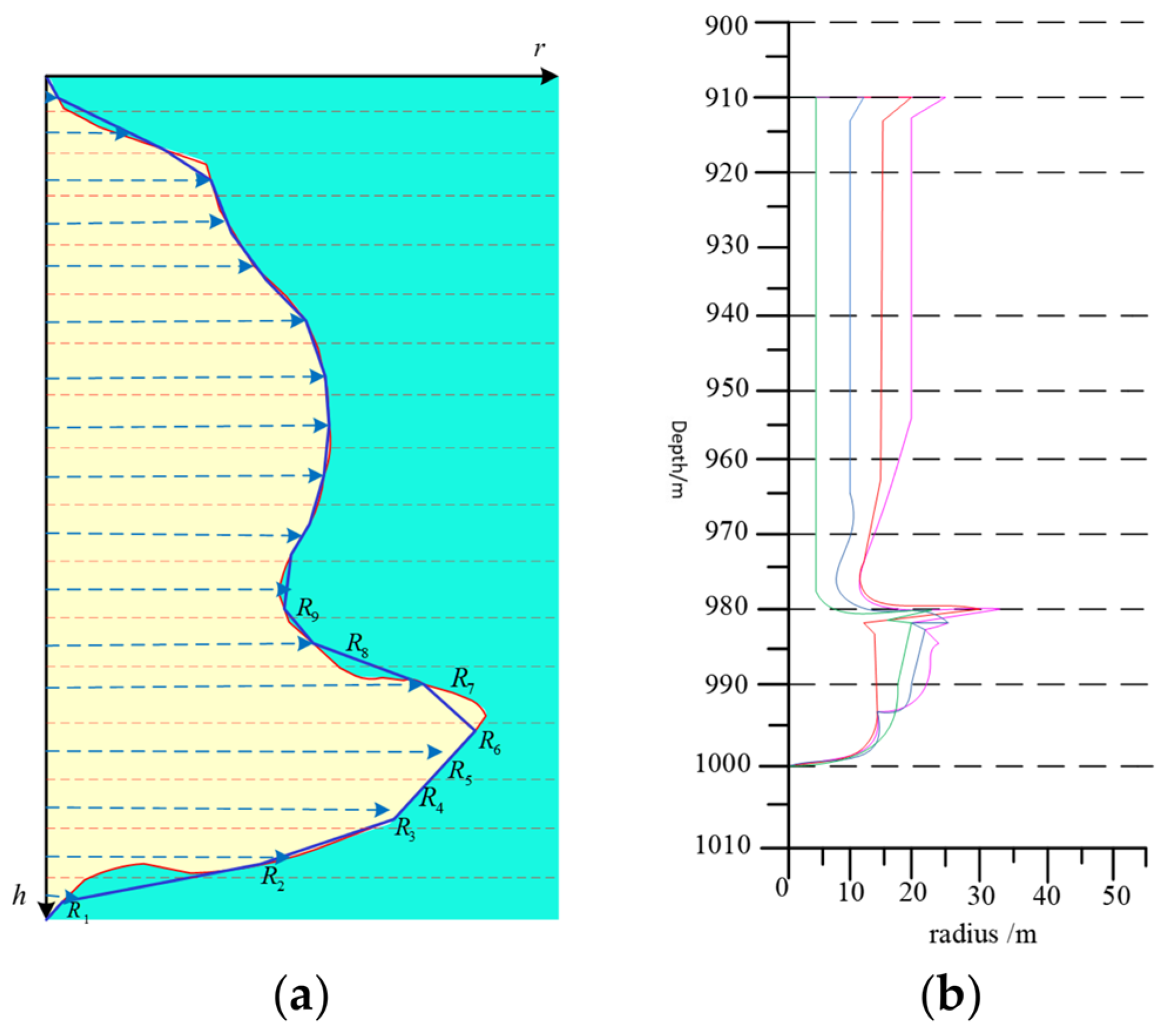
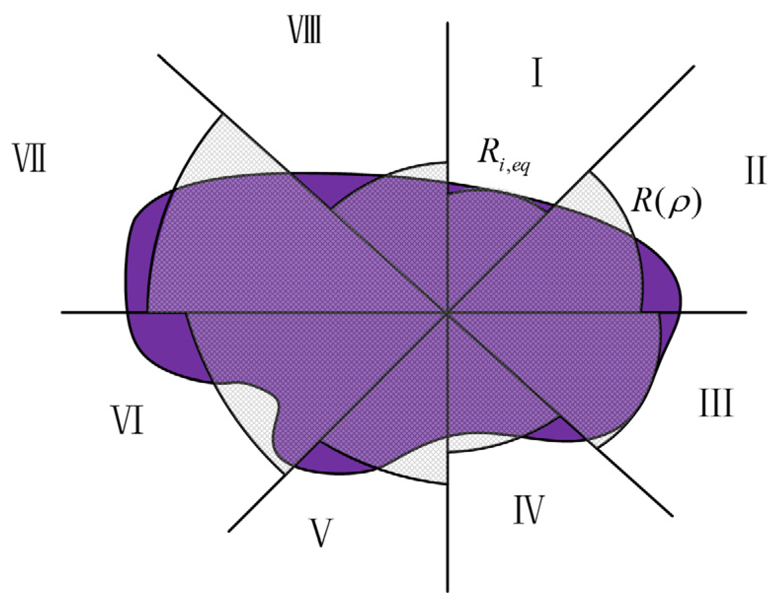
2.2. Cavity Morphology Post-Processing Model

In order to obtain the radius within the sector close to the actual cavity, the same depth sector is assumed to be satisfied:

$$ℛ(\phi )={\left(\frac{K}{\pi }\right)}^{2}a{\phi }^2+\frac{K}{\pi }b\phi +c.$$

(20)

Due to the subsector processing in the calculation process, the equivalent radius R_i,eq is abstracted to facilitate the theoretical calculation, but it also causes the discontinuity of the cavity radius. Therefore, to solve this problem, the cavity morphology needs to be post-processed to make the calculation results closer to the real cavity. First, the radius of the point between two sectors is determined, and the reconciled average of the equivalent radius values in the neighboring sectors is taken:

$$\begin{array}{l}{R}_{\frac{1}{2}}=\frac{2R_{(i+1),eq}{R}_{i,eq}}{R_{(i+1),eq}+R_{i,eq}}\\ R_{-\frac{1}{2}}=\frac{2R_{(i-1),eq}{R}_{i,eq}}{R_{(i-1),eq}+R_{i,eq}}\end{array}.$$

(21)

According to the rule of area equivalence, the following conditions within a sector (taking $-\frac{\pi }{K}$ to $\frac{\pi }{K}$ to be a sector) need to be satisfied:

$$\frac{K}{2\pi }{{\displaystyle \int }}_{-\frac{\pi }{K}}^{\frac{\pi }{K}}{[ℛ(\phi )]}^{2}d\phi ={\left(R_{eq}\right)}^2.$$

(22)

Then, there is the following:

$$\frac{1}{5}{a}^2+\frac{1}{3}{b}^2+c^2+\frac{2}{3}ac={\left(R_{eq}\right)}^2.$$

(23)

Based on Equations (20)–(23), we obtain the following:

$$\begin{array}{l}a=\frac{\beta -\sqrt{{\beta }^2-4\alpha \gamma }}{2\alpha }\\ b=\frac{1}{2}\left(R_{\frac{1}{2}}-R_{-\frac{1}{2}}\right)\\ \mathrm{c}=-a+\frac{1}{2}\left(R_{\frac{1}{2}}+R_{-\frac{1}{2}}\right)\end{array}.$$

(24)

We also obtain the following equation:

$$\begin{array}{l}\begin{array}{l}\alpha =\frac{8}{15}\hfill \\ \beta =\frac{2}{3}\left(R_{\frac{1}{2}}+R_{-\frac{1}{2}}\right)\hfill \end{array}\\ \gamma =\frac{1}{3}\left({\left(R_{\frac{1}{2}}\right)}^2+{\left(R_{-\frac{1}{2}}\right)}^2+R_{\frac{1}{2}}{R}_{-\frac{1}{2}}\right)-{\left(R_{eq}\right)}^2\end{array}.$$

2.3. Mathematical Modeling of Brine Concentration in the Cavity

According to the distribution law of brine flow field and concentration field in the salt cavity [19,20], it is assumed that the brine concentration in the cavity above the inner tube is uniformly distributed in the positive circulation process, and the region below the inner tube is saturated with the brine concentration; therefore, the area above the inner tube is regarded as a control body, and its continuity control equation is as follows [17]:

$$\rho \frac{\partial V}{\partial t}(1-P_N)+\frac{\partial V}{\partial t}{P}_{N}f{C}_N-\left(Q+\frac{\partial V}{\partial t}(P_{N}f-1)\right)C=\frac{\partial (VC)}{\partial t},$$

(25)

where f is the expansion coefficient of the insoluble material (values in the range 1.05–1.38); R is the radius of the salt cavity, m; Q is the injection flow rate, m³/s; V is the volume of the control body, m³; and t is the time, s.

The equation controlling the continuity of the portion of the counter-cycling process above the outer tube to the oil pad is as follows [17]:

$$\rho \frac{\partial V}{\partial t}(1-P_N)-\left(Q-\frac{\partial V}{\partial t}\right)C=\frac{\partial (VC)}{\partial t}.$$

(26)

The transition zone of the portion above the inner tube and below the outer tube is divided into several cell layers. For each cell layer, the conservation of salt mass can be expressed as follows [17]:

$$\frac{\partial \left(C_{h,t}{P}_{N(h,t)}\right)}{\partial h}\mathrm{d}h+\rho \frac{\partial V_{h,t}}{\partial t}(1-P_N)=\frac{\partial \left(C_{h,t}{V}_{h,t}\right)}{\partial t},$$

(27)

where V_h,_t is the volume of microelement, m³.

$$\{\begin{array}{l}{\mu }_{h,t}=Q-\frac{\partial V_{h,t}}{\partial t}\left(h=H_{\mathrm{o}}\right)\hfill \\ \frac{\partial {\mu }_{h,t}}{\partial h}=\frac{\partial V_{h,t}}{\partial t}\left(H_{\mathrm{in}}<h<H_{\mathrm{o}}\right)\hfill \end{array}$$

(28)

3. Results

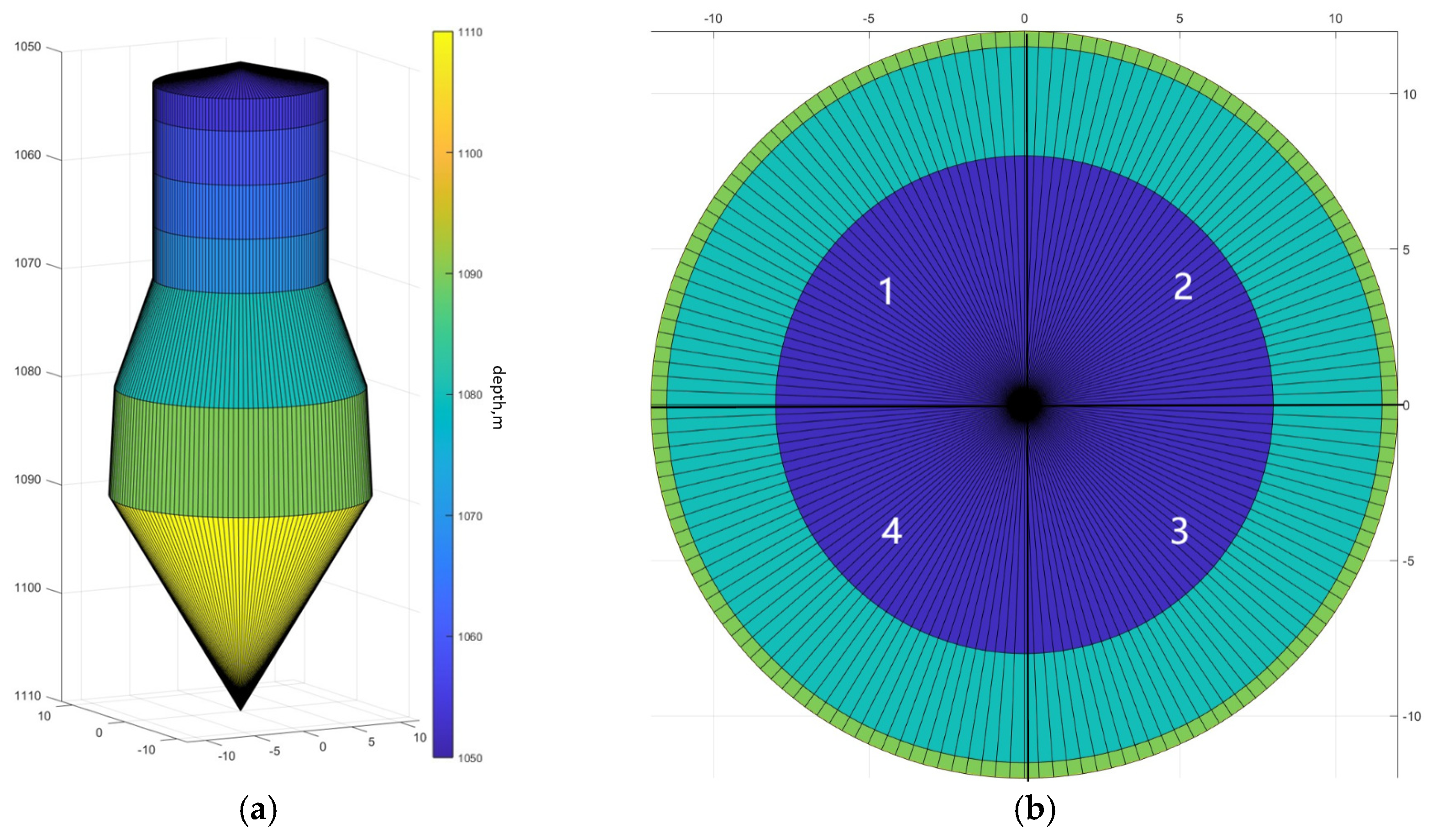
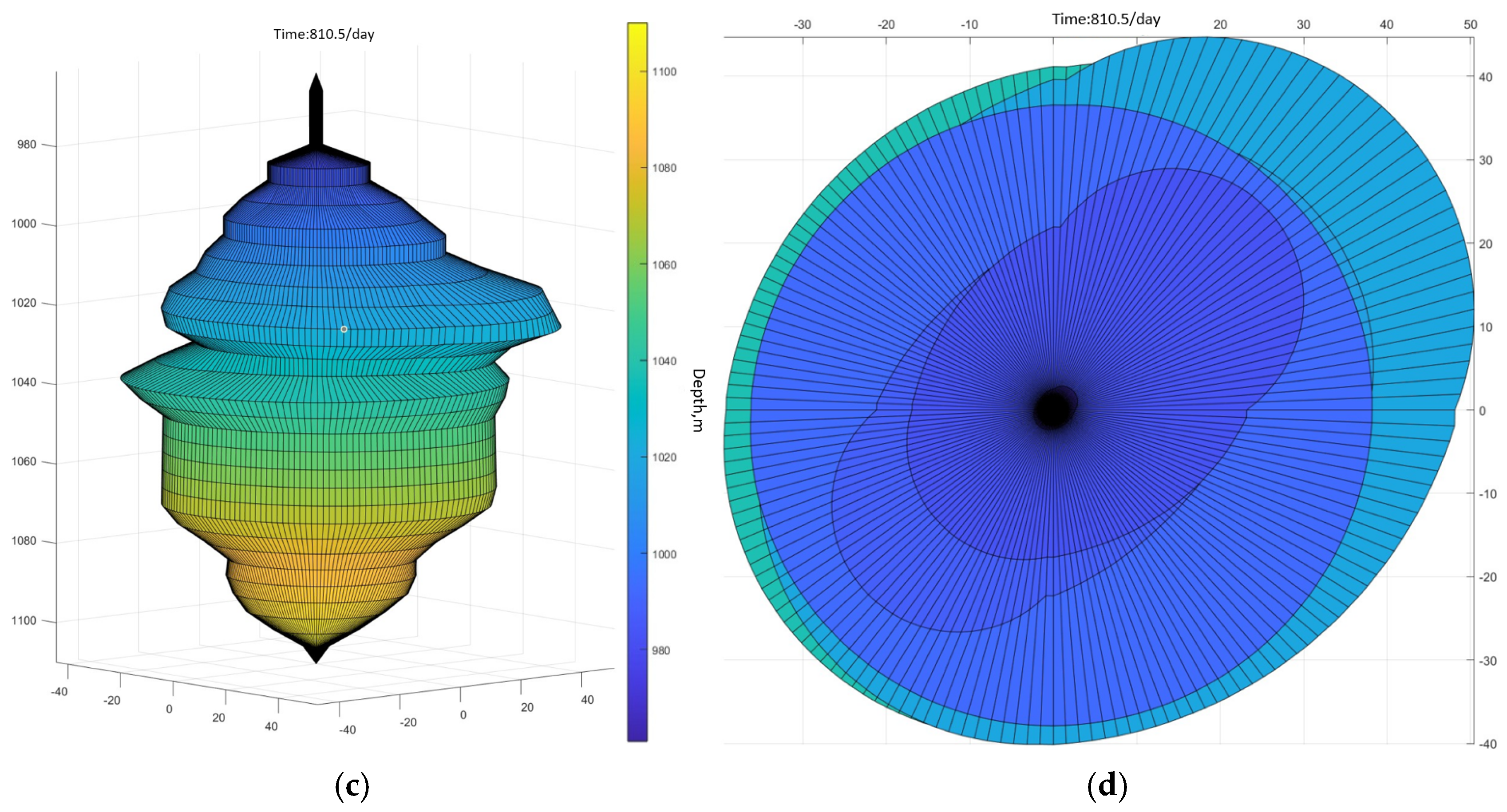
3.1. Cavity Simulation Demonstration

In order to demonstrate the advantages of the software in simulating three-dimensional non-homogeneous water-soluble cavity building, the cavity was divided into four sectors using the basic parameters in

Table 1. Geological parameter table.

Sector Number	1	2	3	4
Insoluble content range	0.5–0.6	0.2–0.3	0.15–0.2	0.8–0.9
Saltstone density range, kg/m3	2400–2500	2300–3200	3600–3800	3000–3200

. Each sector had the same initial profile (as shown in Figure 5a,b). The technical parameters were set as in

Table 2. Technical parameter table.

Lumen Formation Stage	Circulation Mode	Time/Day	Engine Capacity /(m3/d)	Blanket Depth/m	Inner Pipe Depth/m	Outer Pipe Depth/m
1	Positive circulation	150	100	1049	1106	1071
2	Positive circulation	150	100	1035	1079	1056
3	Positive circulation	150	100	1020	1075	1041
4	Reverse circulation	180	100	1000	1046	1070
5	Reverse circulation	150	100	981	1030	1062
6	Reverse circulation	30	100	961	1030	1062

, and in order to better reflect the effect of non-homogeneity on the cavity shape, geologic parameters with a large difference were set and made to show a Gaussian distribution in the salt rock according to the ranges in Table 1, alongside the insoluble matter. The expansion coefficient is set to 1.1, and the temperature is set to 40 °C. The calculated results are shown in Figure 5c,d.

The computational results show that near the depths of 1035 m and 1005 m, the cavity protrudes toward sector 2, indicating that the dissolution rate of sector 2 is significantly higher than that of the other sectors, and at the depth of 1040 m, the cavity protrudes toward sector 4, suggesting that sector 4 has a larger dissolution rate compared to the other sectors at this depth, and for the other depths, the cavity shapes are predominantly elliptical, suggesting that the dissolution rates of the four sectors are similar. The sectors have similar dissolution rates, but there are still some differences. In summary, the software can well reflect the cavity building process of 3D non-homogeneous salt cavern reservoirs.

3.2. Mathematical Model Validation

Using the experimental data of the salt-bearing system distributed in the Fusi section of Funing Formation and combining them with the cavity-making practice of the pilot well of the Jintan Salt Cave Gas Storage Reservoir, the cavity-making operation process is simulated. The salt-bearing wells in the Fusi section of the Funing Group range from 794.8 m to 924.0 m, with a total of 19 layers of 129.2 m. Among them, there are nine layers of salt rock, with a total thickness of 90.1 m; seven layers of salt rock (mud), with a total thickness of 17.2 m; one layer of mud (salt), with a total thickness of 1.7 m; and two layers of mud, with a total thickness of 20.2 m. The specific geologic parameters are presented in

Table 3. Stratigraphy of the Fusi section of Funing Formation.

Floor Number	Well Section (m)	Layer Thickness (m)	Natural Gamma (API)	Compensating for Sound Waves (us/m)	Compensation Density (g/cm3)	Photoelectric Absorption Index (b/ev)	Mud Content (%)	Explanation of Conclusions	Note
1	794.8~809.0	14.2	9.94	226.31	2.06	4.06	3.66	saline rock formation
2	809.0~812.8	3.8	15.90	235.98	2.24	3.69	18.50	saline rock formation	clay
3	812.8~814.9	2.1	79.00	296.38	2.33	3.23	99.90	mudstone layer
4	814.9~828.4	13.5	11.28	232.19	2.09	3.87	4.26	saline rock formation
5	828.4~832.2	3.8	16.77	232.64	2.32	3.35	42.02	saline rock formation	clay
6	832.2~852.6	20.4	10.87	219.9	2.08	3.51	4.08	saline rock formation
7	852.6~856.0	3.4	32.87	231.51	2.16	3.56	19.95	saline rock formation	clay
8	856.0~858.8	2.8	15.37	226.07	2.07	3.76	6.30	saline rock formation
9	858.8~861.5	2.7	20.70	233.04	2.25	3.56	36.69	saline rock formation	clay
10	861.5~871.6	10.1	12.29	224.39	2.06	3.71	4.74	saline rock formation
11	871.6~873.3	1.7	56.51	237.53	2.36	3.21	57.92	mudstone layer	saline
12	873.3~877.5	4.2	14.72	227.65	2.09	3.66	5.96	saline rock formation
13	877.5~878.6	1.1	33.53	234.46	2.28	3.47	20.14	saline rock formation	saline
14	878.6~879.8	1.2	13.94	221.18	2.08	3.70	5.56	saline rock formation
15	879.8~881.0	1.2	23.50	242.25	2.25	3.48	28.45	saline rock formation	clay
16	881.0~884.7	3.7	11.92	228.50	2.08	3.86	4.57	saline rock formation
17	884.7~885.9	1.2	30.65	234.35	2.26	3.44	17.98	saline rock formation	clay
18	885.9~905.9	20.0	12.06	223.22	2.06	3.80	4.63	saline rock formation
19	905.9~924.0	18.1	105.37	279.34	2.56	3.05	99.9	mudstone layer

.

The actual cavity building is divided into three operation stages, of which stages 1 and 2 are the construction stages of the insoluble bottom pit, which adopts the positive cycle method to build the cavity; stages 3 to 5 are the construction stages of the cavity main body, which adopts the reverse cycle method to build the cavity; and finally, stages 6, 7, and 8 are the stages of the establishment of the top of the salt cavern, which still adopts the reverse cycle method to build the cavity. The specific design results of the parameters are shown in

Table 4. Construction statistics of water-soluble cavity creation parameters.

Cavitation Parameters	Circulation Mode	Blanket Depth/m	Outer Pipe Depth/m	Inner Pipe Depth/m	Water Injection Displacement m3/h	Cumulative Luminalization Time/Day
1	Positive circulation	882	890	906	30	46
2	Positive circulation	882	890	906	60	214
3	Reverse circulation	872	880	900	80	306
4	Reverse circulation	862	880	900	80	405
5	Reverse circulation	852	880	900	80	440
6	Reverse circulation	842	860	880	80	532
7	Reverse circulation	832	860	880	80	642
8	Reverse circulation	820	860	880	80	654

.

3.3. Analysis of Results

Comparing the model simulation results of this paper and the prediction results of winUbroNET software, as shown in Figure 6, the contours of the cavity simulated by this software and by winUbro in the three operation phases are largely close to each other, and in comparison with the data in

Table 5. Table of basic process parameters and geological parameters.

Parameter Name	First Stage
Injection time, day	200
Inner pipe depth, m	1095
Outer pipe depth, m	1065
Blanket depth, m	1050
Circulation mode	Positive circulation
Injection flow, m3/s	0.016
Saltstone density, kg/m3	3000–3200
Insoluble content	0.2–0.3
Insoluble expansion coefficient	1.7
Stratigraphical temperature, °C	41
Intercalated saline rock (geology) Dissolution rate, m/s	Lateral solution: 0.00000024472 Paracentesis: 0.00000038444
Sandwich section	1050–1060 m

, the maximum difference of the largest radius is about 2 m at most, and the error is not more than 0.04%. The maximum difference of net volume is about 775 m³, and the maximum error is not more than 0.01%. The simulation results are very close to each other, which verifies the correctness of this software, but the cavity simulated by winUbro is a symmetric three-dimensional image, which does not react to the influence of geological parameters on the simulation of the cavity; on the contrary, due to the effect of geological parameters, the dissolution in each direction is different, so the simulated image is not symmetrical, which is closer to the actual cavity dissolution process, so the accuracy of the simulated cavity contour is higher than that of the cavity contour simulated by winUbroNET.

4. Discussion

According to Theory 2.3 [12], when positive circulation is used, the whole cavity is divided into a main circulation zone and a saturation zone. Within the main circulation zone, the concentration in the cavity is consistent. In order to better explore the influence of each factor on the water-soluble cave-making process in salt caverns, the positive circulation method is adopted, and only one stage is considered for simulation calculation. In order to better reflect the influence of each factor on the cavity dissolution process, each parameter is set to be greater than the recommended value; that is, the dissolution rate will be much faster compared to the actual situation. The specific process parameters and geological parameters are shown in Table 5. In the sensitivity analysis, it is necessary to keep the following parameters unchanged and to only modify one parameter.

Since the purpose of this section is to analyze the influence of various factors on the salt rock water solution cavity building, and there is no need to discuss the non-homogeneity of the cavity building, the cavity building is only divided into 80 layers in this section, the 60th layer is set as an observation point, and there is no more partitioning of the cavity building.

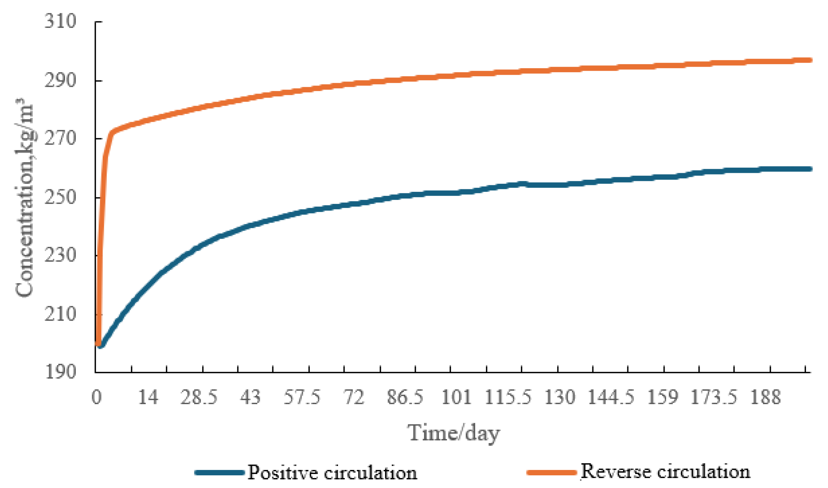
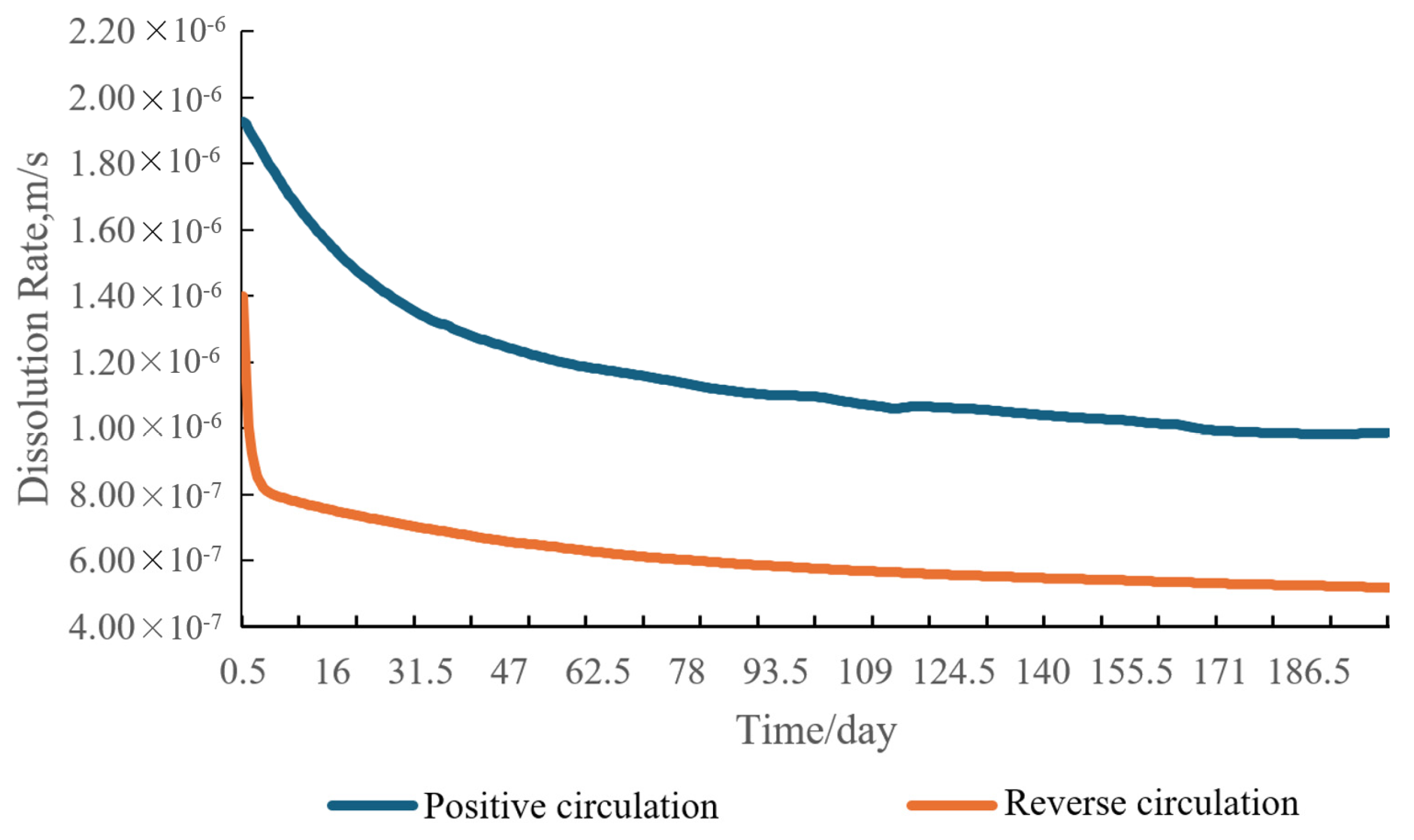
4.1. Circulation Mode Analysis

In the water solution cavity building process for salt cavern reservoirs, the optimization of the process parameters first needs to consider what kind of circulation method should be used to obtain better cavity building efficiency. The results obtained by using the parameters in 3.1 and changing only the circulation method are shown in Figure 7, Figure 8, Figure 9 and Figure 10.

According to the net volume size (as shown in Figure 8), it can be seen that the volume of the reverse circulation is always higher than that of the positive circulation in the process of volume change over time, and the difference is about 10,000 m³ by 188 days, which indicates that the efficiency of the reverse circulation in creating the cavity is obviously better than that of the positive circulation. The reason is that in the process of salt rock dissolution, the location of the discharge outlet of the positive cycle is high, which leads to the easy deposition of high-concentration brine at the bottom of the cavity; therefore, the concentration of the discharged brine is relatively low [28]. The reverse cycle is just the opposite; the outlet position is low, so the bottom of the high concentration of brine can be discharged; thus, the concentration curve in the reverse cycle cavity is always lower than the positive cycle concentration curve (Figure 9), which, in turn, causes the dissolution rate curve to be higher than the positive cycle (Figure 10).

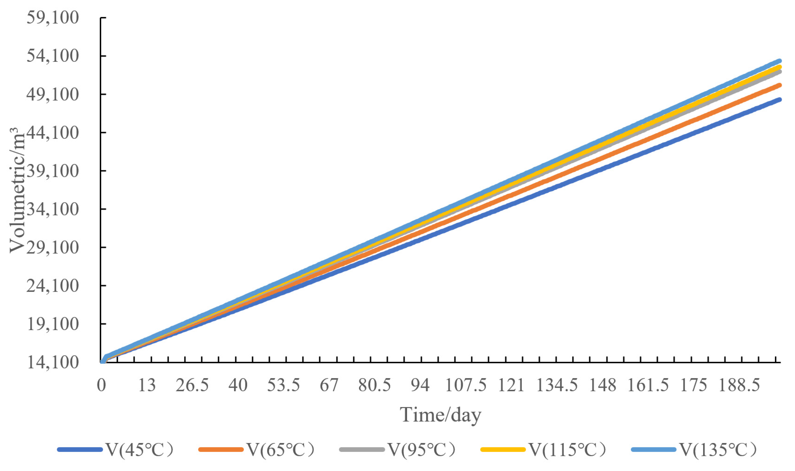
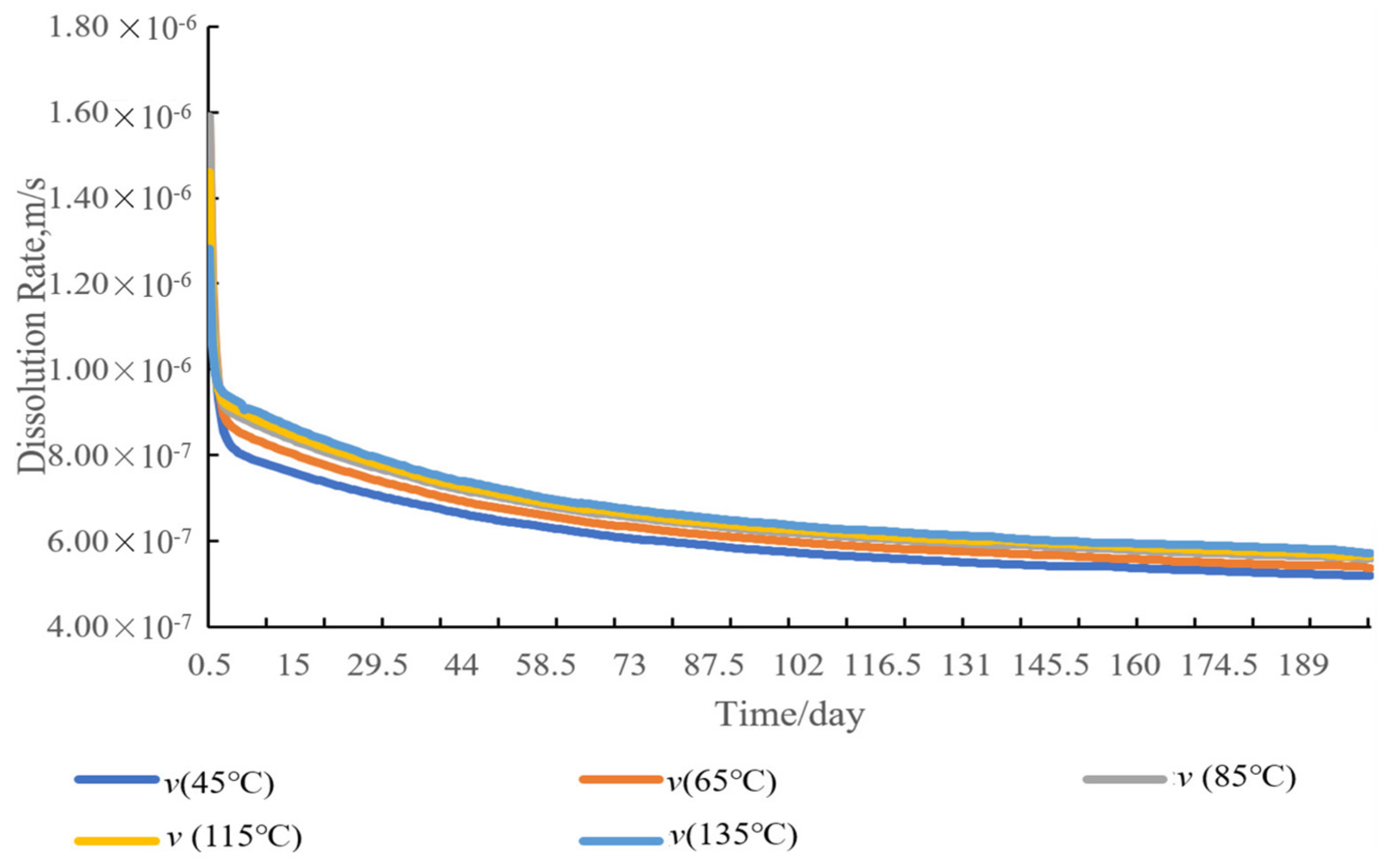
4.2. Temperature Sensitivity Analysis

Other parameters were kept constant, and the changes in the net lumen volume, the concentration within the 60th layer slice, and the dissolution rate are shown in Figure 11, Figure 12 and Figure 13, where the temperatures were 45 °C, 65 °C, 95 °C, 115 °C, and 135 °C, respectively.

As can be seen in Figure 11, as the temperature changes from 45 °C to 135 °C, the temperature increases by a factor of 3, the final net volume of the cavity increases from about 44,000 m³ to about 54,000 m³, the final net volume increase is only about 20%, the final concentration of the cavity increases from 298 kg/m³ to 326 kg/m³, and the final dissolution rate increases from 5.36 × 10⁻⁷ m/s to 5.77 × 10⁻⁷ m/s, which shows that the effect of temperature on the cavity dissolution process is small. The reason is that in the process of salt rock dissolution, the temperature increases, and the salt rock dissolves more easily, which makes the brine concentration in the cavity increase (Figure 12), and the increase in the concentration decreases the salt rock dissolution rate [28]. Therefore, the interaction between the two results in a less pronounced change in the dissolution rate, as seen in Figure 13, resulting in a smaller change in the net volume of the cavity with increasing temperature.

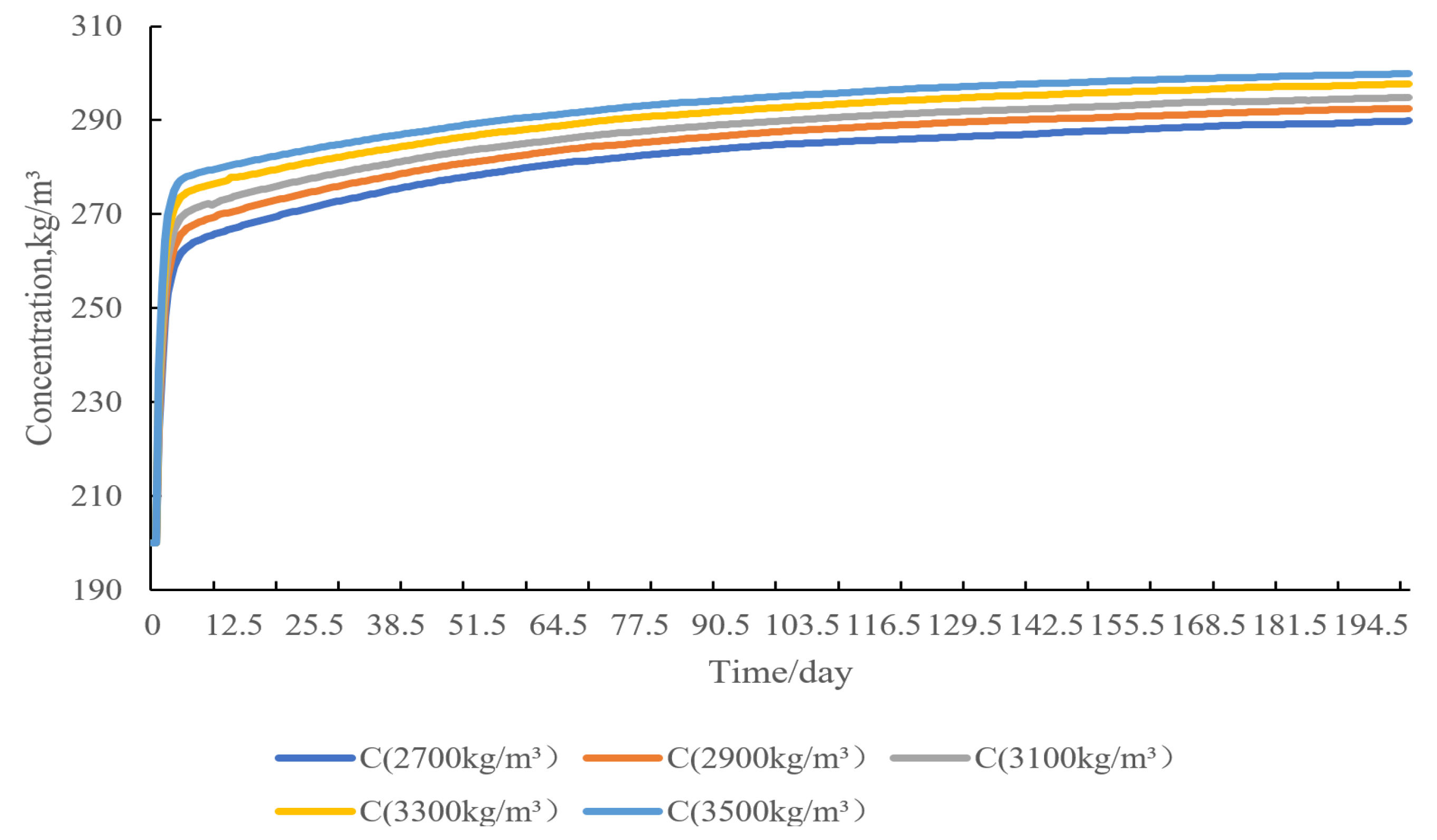
4.3. Saltstone Density Sensitivity Analysis

Other parameters were kept constant, and when the full density of salt rock was 2600–2800 kg/m³, 2800–3000 kg/m³, 3200–3400 kg/m³, 3400–3600 kg/m³, 3400–3600 kg/m³, and 3600–3800 kg/m³, respectively, the changes of the net cavity volume, the concentration within the 60th layer of the slices, and the dissolution rate are shown in Figure 14, Figure 15 and Figure 16.

The effect of salt rock density on the cavity building of salt rock water dissolution is slightly larger than that of temperature. From Figure 14, Figure 15 and Figure 16, it can be seen that with the increase in salt rock density, the cavity concentration gradually becomes larger, and the dissolution rate and net volume gradually become smaller. In addition, Figure 14, Figure 15 and Figure 16 shows that with every 200 kg/m³ increase in the density value of salt rock, the final net volume of the cavity increases by about 1600 m³, the final cavity concentration increases by an equal amount of about 2 kg/m³, and the dissolution rate decreases by an equal amount of about 1 × 10⁻⁷ m/s. This is because the dissolution rate is approximately linear with the density, and the increase in the magnitude of the change of the net volume in Figure 16 is also almost the same, as shown in Figure 16. This is consistent with the conclusion of Ma Hongling et al. and again verifies the accuracy of the present model [28]. Therefore, an equal increase in the density of salt rock, with other conditions unchanged, will result in a roughly equal decrease in the net volume of the cavity.

4.4. Sensitivity Analysis of Insoluble Matter Content

Other parameters were kept constant with different insoluble content settings of 0.1–0.2, 0.3–0.4, 0.5–0.6, 0.6–0.7, and 0.8–0.9, and the changes in net lumen volume, concentration within the 60th layer of slices, and dissolution rate are shown in Figure 17, Figure 18 and Figure 19.

The change in insoluble content is very sensitive to the influence of the cavity dissolution process. When the insoluble content is increasing, the cavity volume also continues to become larger, while the magnitude of the increase also continues to become larger; specifically, when the insoluble content increased from 0.15 to 0.85, the final net volume changed from 45,148.81 m³ to 111,831.3 m³, an increase of more than double; however, the actual volume gradually decreased from an initial 26,393.5 m³ to 14,660.05 m³ (Figure 17). This shows that when the insoluble content increases, the salt rock is more easily dissolved, and at the same time, the quantity of substances that can be dissolved into the water will decrease, making the brine concentration in the cavity decrease (Figure 18). Under other conditions, the two are superimposed on each other to make the rate of dissolution increase (Figure 19), but the increase in the insoluble content will result in an insoluble accumulation of volume; thus, the actual volume of the cavity is gradually reduced, so with the increase in insoluble content, the actual cavity volume gradually decreases.

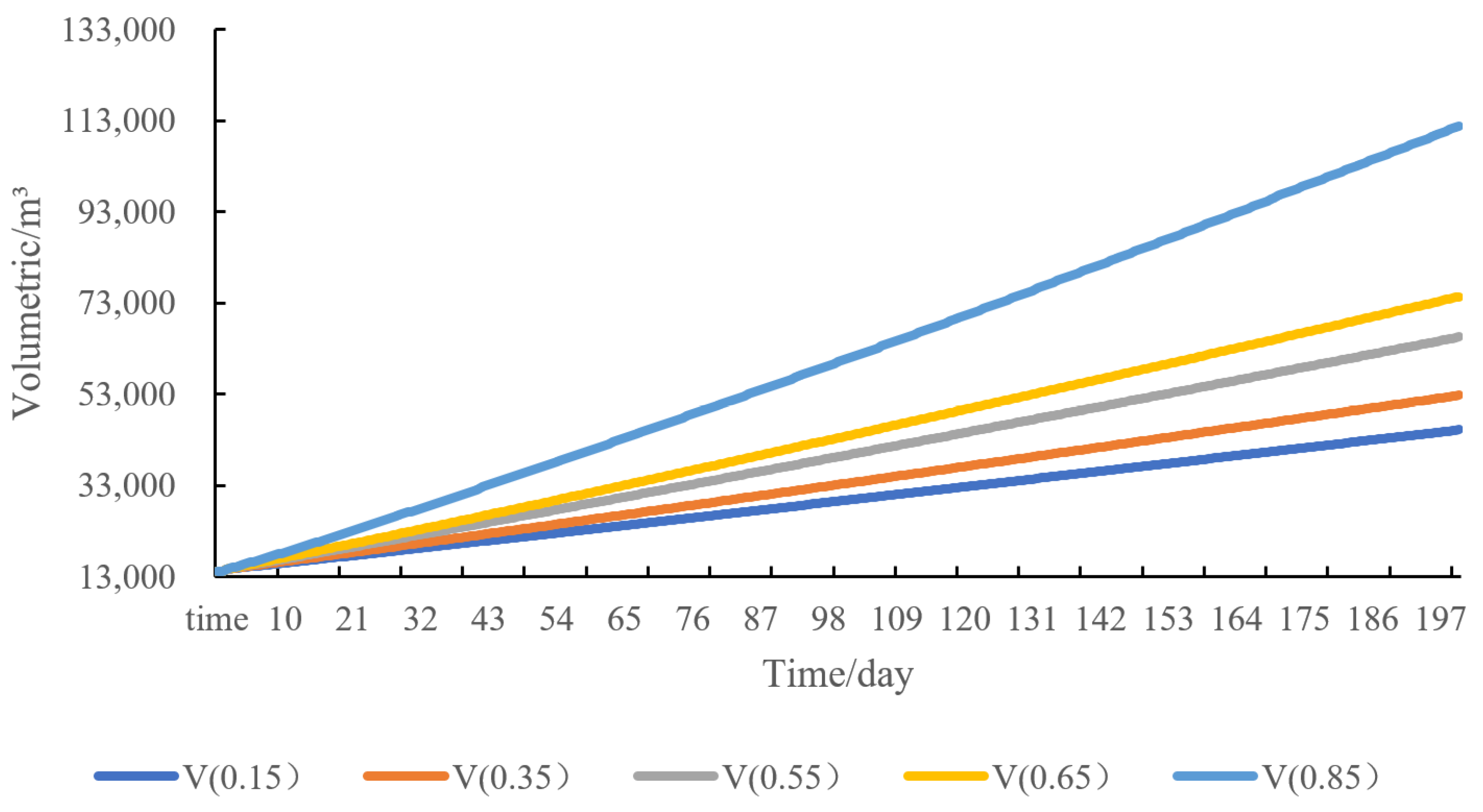
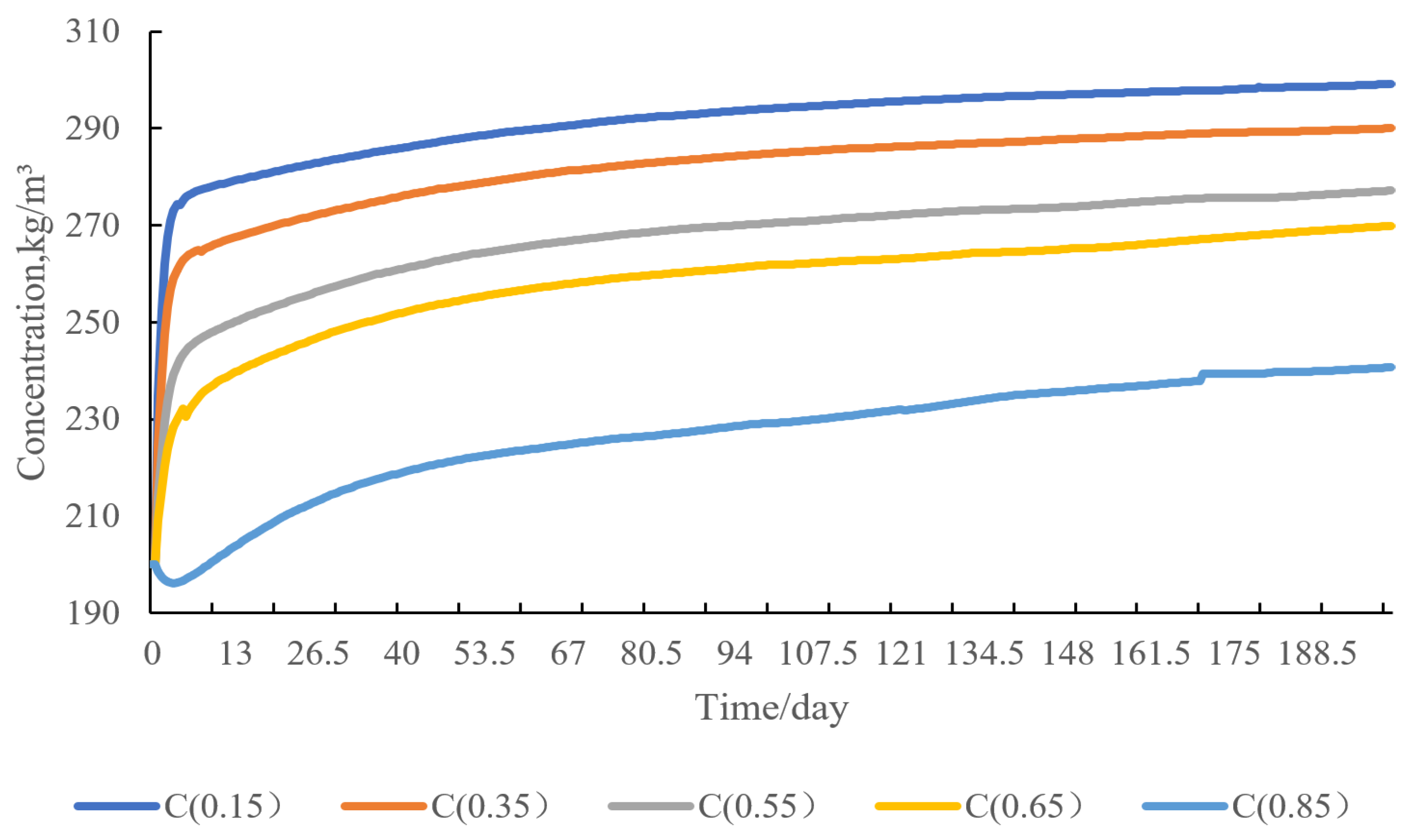
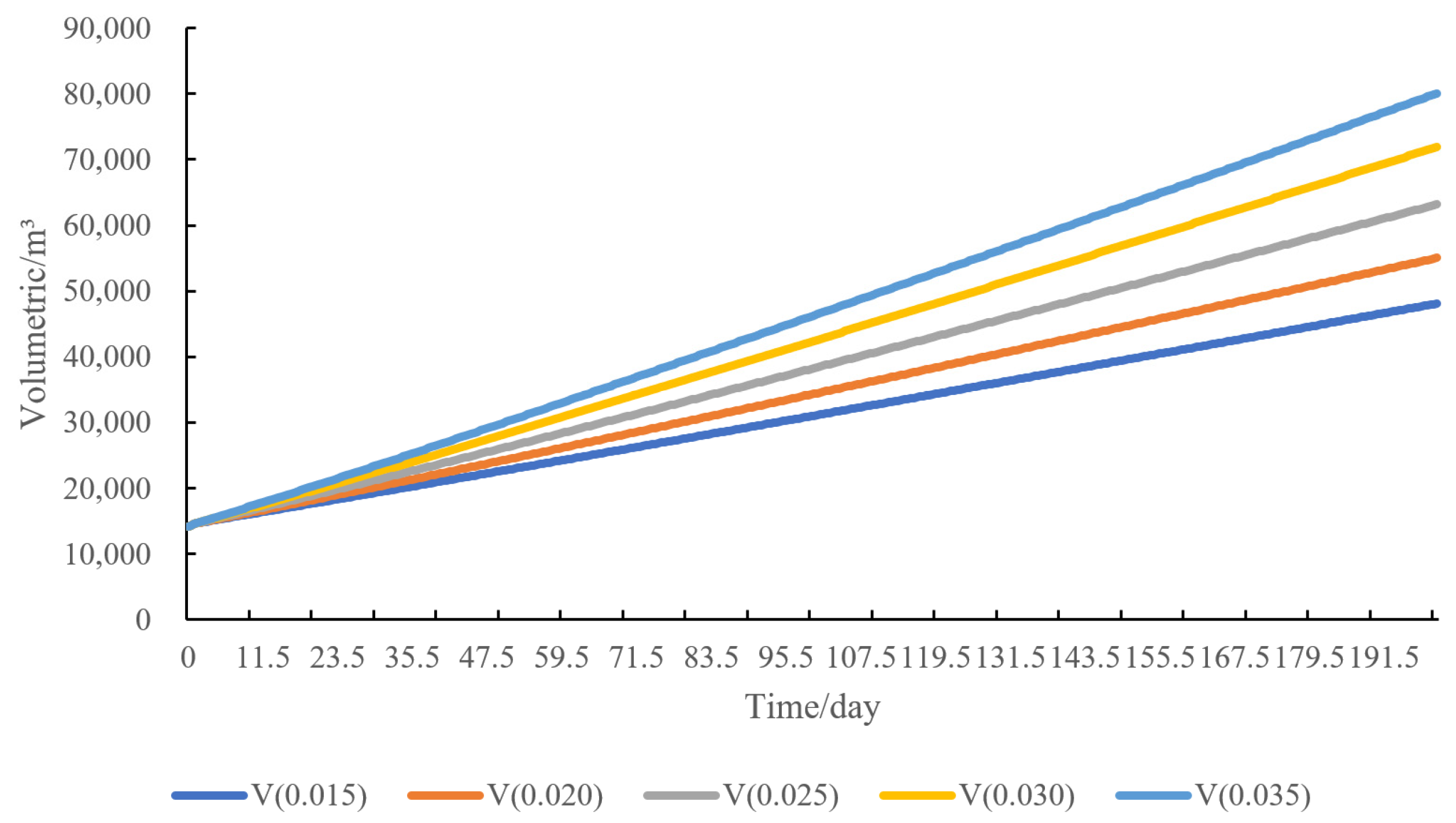
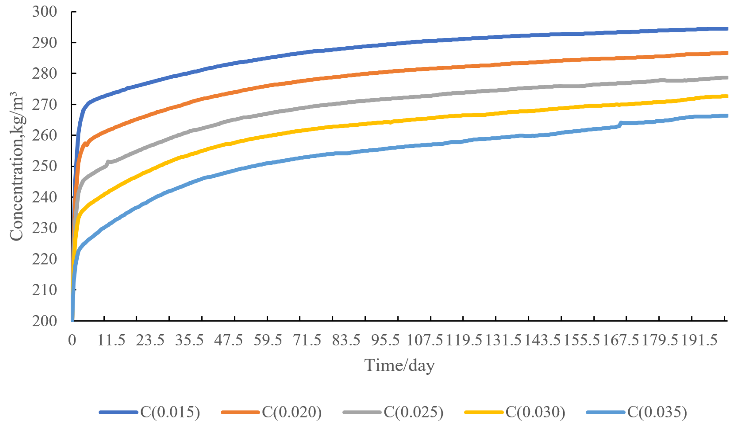
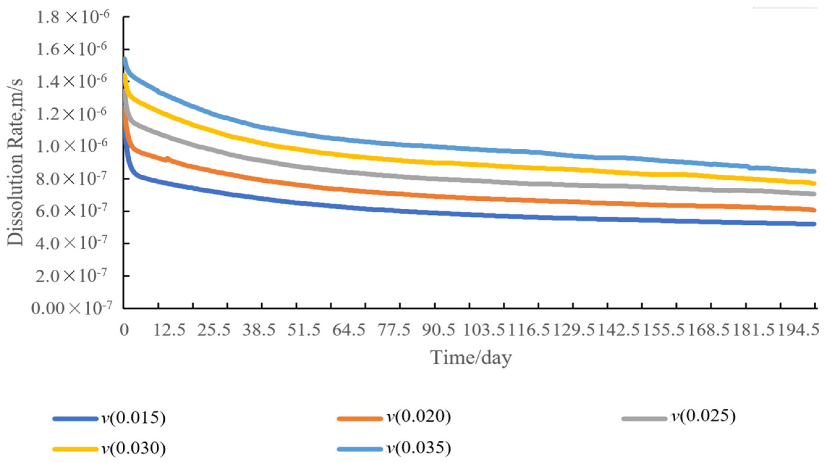
4.5. Sensitivity Analysis of Water Injection Volume

The parameters were kept constant, and the water injection flow rates were set to 0.015 m³/s, 0.020 m³/s, 0.025 m³/s, 0.030 m³/s, and 0.035 m³/s. Changes in the net lumen volume, the concentration within the 60th layer of slices, and the dissolution rate are shown in Figure 20, Figure 21 and Figure 22.

The water injection flow rate is more sensitive to the cavity dissolution process. From Figure 20, Figure 21 and Figure 22, it can be seen that with the increase in the water injection flow rate, the net volume of the cavity shows a trend of equal increase; for example, the water injection flow rate increasing from 0.015 m³/s to 0.035 m³/s. Every increase of 0.005 m³/s corresponds to an increase of about 8000 m³ in the net volume. As the water injection flow rate increases, the concentration in the chamber gradually decreases, making the dissolution rate also increase. Therefore, in order to shorten the cavity building cycle within a reasonable range, a large-diameter center tube should be selected as often as possible to increase the water injection flow rate.

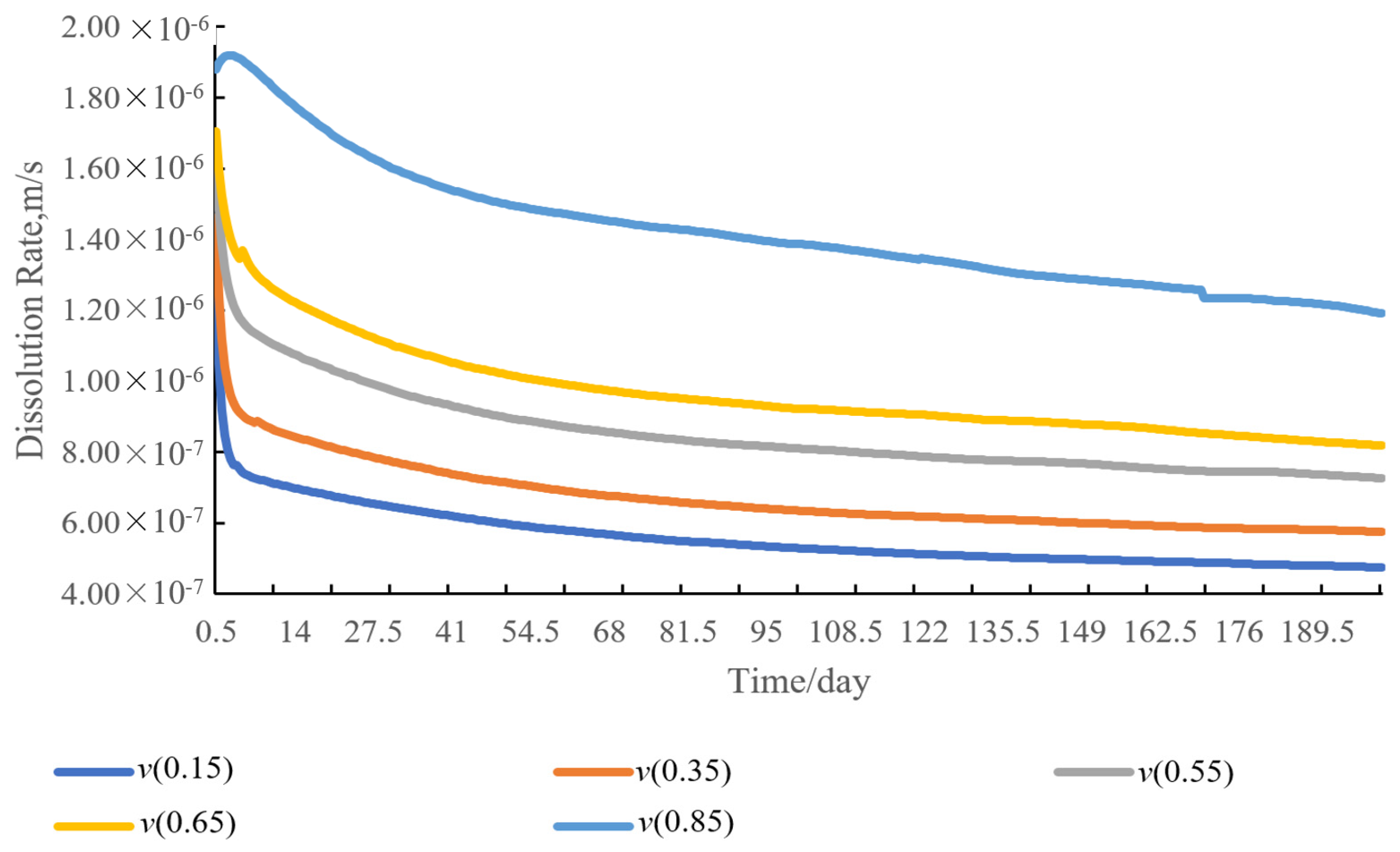
4.6. Sensitivity Analysis of Dissolution Rate of Entrained Salt Rocks

Other parameters were kept constant, and the dissolution rate of the intercalated salt rock was changed to 2/3, 1/2, 1/3, 1/5, and 1/6 of the dissolution rate of the salt rock, respectively. The changes in the net cavity volume, the concentration in the 60th layer of the slice, and the dissolution rate are shown in Figure 23, Figure 24 and Figure 25.

As can be seen in Figure 23, the net volume of the cavity gradually decreased with the decrease in the dissolution rate of the intercalated salt rock, but the effect of the change in the dissolution rate of the intercalated salt rock on the dissolution of the cavity was not sensitive when compared to other factors. Although the final concentration in the cavity decreased from about 293 kg/m³ to about 248 kg/m³ due to the decrease in the dissolution rate of the intercalated salt rock, the amount of NaCl and other dissolved substances became smaller (Figure 24) and the dissolution rate decreased from 5.3 × 10⁻⁷ m/s to 1 × 10⁻⁷ m/s. The difference in the dissolution rate was not as large as the difference in the concentration change. The reason is that the dissolution rate of the salt rock containing the intercalation is smaller than the dissolution rate of the salt rock on the upper and lower sides, and with the dissolution of the salt rock causing the wall to be concave, the tilt angle of one side of the salt rock wall increases or decreases, which ultimately causes the difference in the dissolution rate to be less than the difference in the concentration change. In addition, when the angle over π/2 of this critical value changes in accordance with the rate of change law, as reflected in Figure 25, the dissolution rate suddenly decreases, and with the decline in the dissolution rate of the salt rock containing the interlayer, the impact increases; thus, the 60th layer, with the sudden decline in the dissolution rate of the salt rock, is constantly advancing.

5. Conclusions

In this paper, a three-dimensional non-homogeneous salt cavern reservoir water-soluble cavity building model is established using the equivalent line segment method, taking into account the insoluble content, salt rock density, water injection flow rate, entrapment, and temperature. The following points of understanding were obtained in the research process:

(1)

The equivalent line segment method is used to describe the cavity contour, and compared with the equivalent tangent point method, which moves the contour points in the horizontal direction by fixing the vertical height, the contour points can be moved in both the horizontal direction and in the vertical direction using this method to avoid the drawbacks of a jagged cavity contour appearing, brought about by the equivalent tangent point method.

(2)

A three-dimensional non-homogeneous salt cavern reservoir water solution cavity model was established, and the cavity was divided into several sectors in the horizontal direction and several layers in the vertical direction. The geological parameters, such as the density of the salt rock and the insoluble content in each sector, satisfied the Gaussian distribution, and the temperature varied linearly according to the number of layers in the vertical direction. The numerical simulation software for the water solution cavity construction of a three-dimensional non-homogeneous salt cavern reservoir was prepared using MATLAB R2023b software.

(3)

Using the experimental data of the salt system distribution in the Fusi section of the Funing Group and the parameters of the cavity expansion results of the salt cavity of the Jintan reservoir’s early well No. 52, the numerical simulation results of the cavity produced by this software, CALES, and winUbro were compared. The results show that the cavity shapes simulated by this software maintain a high degree of consistency with the actual cavity shapes, and at the same time, they demonstrate a high degree of accuracy in terms of maximum radius and volume error. This excellence is mainly attributed to the 3D non-homogeneous model introduced in the software, which successfully captures and accurately reflects the effect of non-homogeneous geology on the cavity shape.

(4)

The time standard for completing the cavity plays a decisive role in the cavity expansion process. In particular, in practical engineering applications, the time of cavity expansion not only affects the overall project schedule but also directly relates to the economic efficiency and safety management of the dissolution process. Under the requirement of rapid completion of cavity construction, the model proposed in this study can predict the cavity expansion time more accurately and ensure the completion of cavity construction within the optimal time, thus reducing the project cost and improving the efficiency of resource utilization. Therefore, the reasonable setting and accurate prediction of time standards are crucial to the success of cavity construction.

References

1. Wu, H.; He, Y.; Zhou, Y.; Ji, S.; Luo, Y. Comparison and Selection of Natural Gas Peaking Methods. Nat. Gas Oil 2009, 27, 5–9+58+63. [Google Scholar]
2. Zhou, X. Effective natural gas peaking and storage technology—Underground gas storage. Nat. Gas Ind. 2013, 33, 95–99. [Google Scholar]
3. Ding, G.; Jing, L.; Ren, Y.; Zhao, X.; Ran, L. Suggestions for building China’s natural gas peaking reserve and emergency response system. Nat. Gas Ind. 2009, 29, 98–100+144. [Google Scholar] [CrossRef]
4. Wang, F.; Wang, D. Peaking technology of underground gas storage for gas pipeline. Pet. Plan. Des. 2011, 22, 28–30. [Google Scholar]
5. Korzeniowski, W.; Skrzypkowski, K.; Poborska-Młynarska, K. The Idea of the Recovery of Municipal Solid Waste Incineration (MSWI) Residues in Kłodawa Salt Mine S.A. by Filling the Excavations with Self-Solidifying Mixtures. Arch. Min. Sci. 2023, 63, 553–565. [Google Scholar] [CrossRef] [PubMed]
6. Nolen, J.S.; Von Hantlemann, O.; Meisters, S.; Kleinitz, W.; Heiblinger, J. Numerical simulation of the solution mining process. In Proceedings of the SPE European Spring Meeting, Amsterdam, The Netherlands, 29 May 1974; Society of Petroleum Engineers: Amsterdam, The Netherlands, 1974. [Google Scholar]
7. Reda, D.C.; Russo, A.J. Experimental studies of saltcavity leaching by freshwater injection. SPE Prod. Eng. 1986, 1, 82–86. [Google Scholar] [CrossRef]
8. Kunstman, A.S.; Urbanczyk, K.M. UBRO-a computer model for designing salt cavern leaching process developed at CHEMKOP. In SMRI Meeting Paper; Solution Mining Research Institute: Paris, France, 1990; pp. 167–172. [Google Scholar]
9. Ban, F.; Gao, S.; Shan, W.; Xiong, W. Modeling of rock salt erosion in water-soluble gas storage reservoirs. J. Liaoning Univ. Eng. Technol. 2005, 24 (Suppl. S2), 102–104. [Google Scholar]
10. Grüschow, N.; Rembe, M. Numerical modeling of potash solution mining caverns. In Proceedings of the Solution Mining Research Institute Fall 2012 Technical Conference, Bremen, Germany, 1–2 October 2012. [Google Scholar]
11. Wang, T.; Yang, C.; Li, J.; Li, J.; Shi, X.; Ma, H. Failure Analysis of Overhanging Blocks in the Walls of a Gas Storage Salt Cavern: A Case Study. Rock Mech. Rock Eng. 2016, 50, 125–137. [Google Scholar] [CrossRef]
12. Li, J.; Shi, X.; Yang, C.; Li, Y.; Wang, T.; Ma, H.; Shi, H.; Li, J.; Liu, J. Repair of irregularly shaped salt caven gas storage by re-leaching under gas blanket. J. Nat. Gas Sci. Eng. 2017, 45, 848–859. [Google Scholar] [CrossRef]
13. Li, J.; Tang, Y.; Shi, X.; Xu, W.; Yang, C. Modeling the construction of energy storage salt caverns in bedded salt. Appl. Energy 2019, 255, 113866. [Google Scholar] [CrossRef]
14. Katarzyna, C. Refinements to Cavity Morphology Predictions Under Various Operational Conditions. J. Nat. Gas Sci. Eng. 2021, 78, 103413. [Google Scholar]
15. Cyran, K.; Kowalski, M. Shape Modelling and Volume Optimisation of Salt Caverns for Energy Storage. Appl. Sci. 2021, 11, 423. [Google Scholar] [CrossRef]
16. Li, J.; Wang, Z.; Zhang, S.; Shi, X.; Xu, W.; Zhuang, D.; Liu, J.; Li, Q.; Chen, Y. Machine-learning-based capacity prediction and construction parameter optimization for energy storage salt caverns. Energy 2022, 254, 124238. [Google Scholar] [CrossRef]
17. Wang, T.; Ding, Z.; He, T.; Xie, D.; Liao, Y.; Chen, J.; Zhu, K. Stability of the horizontal salt cavern used for different energy storage under varying geological conditions. J. Energy Storage 2024, 84, 110817. [Google Scholar] [CrossRef]
18. Saberian, A. Study on Mixing in Water-Brine Systems; Solution Mining Research Institute: Paris, France, 1971. [Google Scholar]
19. Saberian, A.; Von Schonfeldt, H.A. Convective mixing of water with brine around the periphery of vertical tube. In Proceedings of the 1973 Fourth Symposium on Salt, Houston, TX, USA, 8–12 April 1973. [Google Scholar]
20. Saberian, A. Cavity Development in a Three Layer Bedded Salt Model; Solution Mining Research Institute: Paris, France, 1977. [Google Scholar]
21. Saberian, A. SALGAS User’s Manual, Volume 1—Theories, Formulas & Program Description; SMRI Research Project Report No. 84-003-SMRI; Solution Mining Research Institute: Paris, France, 1984. [Google Scholar]
22. Podio, A.L.; Saberian, A. Optirnization of solution mining operations. In Proceedings of the 5th International Symposium on Salt-Northem Ohio Geological Society, Hamburg, Germany, 29 June 1979; pp. 87–103. [Google Scholar]
23. Ehgartner, B.L.; Sobolik, S.R. Analysis of Cavern Shapes for the Strategic Petroleum Reserve; Technical Report; Sandia National Laboratories (SNL): Albuquerque, NM, USA; Livermore, CA, USA, 2006. [CrossRef]
24. Wang, T.; Yang, C.; Shi, X.; Ma, H.; Li, Y.; Yang, Y.; Daemen, J.J.K. Failure analysis of thick interlayer from leaching of bedded salt caverns. Int. J. Rock Mech. Min. Sci. 2015, 73, 175–183. [Google Scholar] [CrossRef]
25. Edler, D. Numerical simulation of cavern shape development during product withdrawal with fresh water theory and case study. In Proceedings of the 9th International Symposium on Salt, Beijing, China, 3 September 2009. [Google Scholar]
26. Saberian, A. Numerical Simulation of Development of Solution-Mined Storage Cavities; Texas University: Austin, TX, USA, 1974. [Google Scholar]
27. Kunstman, A.; Urbanczyk, K.; Mlynarska, K.P. Solution Mining in Salt Deposits-Outline of Recent Development Trends; AGH University of Science and Technology: Krakow, Poland, 2007; pp. 106–118. [Google Scholar]
28. Ma, H.; Chen, F.; Yang, C.; Shi, X.; Zhang, Z. Experimental study on dissolution rate of deep salt rocks. Min. Ind. Res. Dev. 2010, 30, 9–13. [Google Scholar] [CrossRef]
Figure 1. Schematic diagram of equivalent tangent point method section: (a) equivalent cut-point method; (b) SANSMIC calculation results. Different colored line segments indicate the position of the cavity contour at each step size.
Processes 12 01124 g001
Figure 2. Schematic diagram of equivalent line segment method.
Processes 12 01124 g002
Figure 3. Incremental diagram.
Processes 12 01124 g003
Figure 4. Schematic diagram of transverse division of cavity.
Processes 12 01124 g004
Figure 5. Cavity simulation example of salt cavern gas storage: (a) side view of initial cavity; (b) top view of initial cavity; (c) side view of calculation results; (d) top view of calculation results.
Processes 12 01124 g005aProcesses 12 01124 g005b
Figure 6. Comparison of simulation results of different operation stages of salt cavern gas storage reservoirs. (ac) are the cavity morphology diagrams of the simulation results of the three operational phases of winUbro, and (df) are the cavity morphology diagrams of the simulation results of the three operations of the model built in this paper.
Processes 12 01124 g006
Figure 7. Positive and negative circulation cavity shape diagram: (a) positive circulation; (b) reverse circulation.
Processes 12 01124 g007
Figure 8. Positive and negative cycle volume comparison chart.
Processes 12 01124 g008
Figure 9. Positive and negative cycle layer 60 concentration comparison chart.
Processes 12 01124 g009
Figure 10. Comparison of dissolution rates of layer 60 in positive and negative cycles.
Processes 12 01124 g010
Figure 11. Net volume change at different temperatures.
Processes 12 01124 g011
Figure 12. Concentration change in layer 60 at different temperatures.
Processes 12 01124 g012
Figure 13. Variation of dissolution rate in layer 60 at different temperatures.
Processes 12 01124 g013
Figure 14. Plot of net volume change for different salt rock densities.
Processes 12 01124 g014
Figure 15. Variation of layer 60 concentration at different salt rock densities.
Processes 12 01124 g015
Figure 16. Variation of dissolution rate in layer 60 at different salt rock densities.
Processes 12 01124 g016
Figure 17. Net volume variations at different insoluble matter contents.
Processes 12 01124 g017
Figure 18. Concentration variation of layer 60 under different insoluble contents.
Processes 12 01124 g018
Figure 19. Dissolution rate of layer 60 under different insoluble contents.
Processes 12 01124 g019
Figure 20. Concentration variation of layer 60 under different water injection flow rates.
Processes 12 01124 g020
Figure 21. Dissolution rate variation of layer 60 under different water injection flow rates.
Processes 12 01124 g021
Figure 22. Volume change chart under different water injection flow rates.
Processes 12 01124 g022
Figure 23. Volume variation diagrams for different interlayer dissolution rates.
Processes 12 01124 g023
Figure 24. Concentration variation of layer 60 under different interlayer dissolution rates.
Processes 12 01124 g024
Figure 25. Dissolution rate variation of layer 60 under different interlayer dissolution rates.
Processes 12 01124 g025