Towards Reliable Prediction of Performance for Polymer Electrolyte Membrane Fuel Cells via Machine Learning-Integrated Hybrid Numerical Simulations

Abstract

For mitigating global warming, polymer electrolyte membrane fuel cells have become promising, clean, and sustainable alternatives to existing energy sources. To increase the energy density and efficiency of polymer electrolyte membrane fuel cells (PEMFC), a comprehensive numerical modeling approach that can adequately predict the multiphysics and performance relative to the actual test such as an acceptable depiction of the electrochemistry, mass/species transfer, thermal management, and water generation/transportation is required. However, existing models suffer from reliability issues due to their dependency on several assumptions made for the sake of modeling simplification, as well as poor choices and approximations in material characterization and electrochemical parameters. In this regard, data-driven machine learning models could provide the missing and more appropriate parameters in conventional computational fluid dynamics models. The purpose of the present overview is to explore the state of the art in computational fluid dynamics of individual components of the modeling of PEMFC, their issues and limitations, and how they can be significantly improved by hybrid modeling techniques integrating with machine learning approaches. Furthermore, a detailed future direction of the proposed solution related to PEMFC and its impact on the transportation sector is discussed.

1. Introduction

Fossil fuels, such as coal, oil, and natural gas, have been the primary sources of energy over the past 50 years, despite their significant impact on increasing CO₂ emissions and contributing to global warming [1,2]. This trend is unlikely to stop owing to the growing population and economic development unless a reliable and sustainable energy source replaces fossil fuels [3]. According to the modified Klass model [4], the depletion of oil, coal, and natural gas will take approximately 35, 107, and 37 years, respectively. The fuel infrastructure cannot be constructed overnight, even in light of the dire situation, because the process is costly and slow.

In this regard, hydrogen is seen as a suitable alternative to conventional fuels as both an energy source and carrier that could help alleviate the detrimental impacts of fossil fuel combustion on the environment [5,6]. Hydrogen utilizes electrochemical reactions to convert it into fuel and directly oxidize it for generating electricity [5]. Based on the electrolyte and working temperature, hydrogen fuel cells are classified as low temperature (20–100 °C), medium temperature (200–300 °C), and high temperature (600–1500 °C) fuel cells [7]. Low-temperature fuel cells have made notable advancements in transportation applications because of their rapid startup, compact size, and lighter weight in comparison to high-temperature fuel cells [8]. Proton exchange membrane fuel cells (PEMFCs) and alkaline fuel cells (AFCs) are among the most common types of low-temperature fuel cells. Both PEMFCs and AFCs are relatively low cost, though there is a lack of waste heat recovery. PEMFCs require costly platinum as an electrode and are prone to carbon monoxide (CO) and sulfur (S) poisoning, whereas AFCs require pure hydrogen (H₂) and oxygen (O₂) in addition to a potential risk of carbon dioxide (CO₂) poisoning [9]. However, based on their power densities, efficiency, and sensitivity to fuel impurities, PEMFCs are the most prominent options for low-temperature fuel cells [9,10,11]. PEMFCs have the potential to satisfy the power demands of various sectors, such as transportation (e.g., hybrid electric vehicles (HEV) [12], ships [13,14], and stationary and portable power generation [15]. However, PEMFCs have several shortcomings, including limited power density (<3 kW∙L⁻¹), low durability (<5000 h) [16], and high material cost [17], which hinder their market competitiveness [18]. Hence, further research is required to address the following issues to achieve the potential of PEMFCs:

Water management: Maintaining an appropriate amount of water inside the cell during PEMFC system operation is challenging because good proton conductivity must be achieved without compromising the performance by flooding the reaction site [19].

Thermal issue: In most cases, PEMFCs have an energy efficiency of approximately 50% because they produce waste heat almost equal to their electric power output [20]. Moreover, to maintain good proton conductivity, the temperature needs to be kept below 80 $\mathrm{℃}$ to prevent dehydration, and temperatures below 60$℃$ can lead to water condensation and cell flooding [21].

Cost and durability: The high Pt catalyst loading and membrane account for almost 80% of the cost of the PEMFC stack [22]. In addition, the materials used must have adequate temperature and humidity tolerance as well as suitable mechanical strength to withstand compression [23]. The degradation of materials and their impact on cell performance must also be considered [24].

To address the aforementioned issues, various experimental studies [25,26,27,28,29,30] have been conducted. However, experiments are expensive, sequential, time-consuming [31], limited to laboratory-scale models, and can be employed to measure only one quantity at a time, which is not convenient for improving the performance over existing designs [32]. By contrast, computational fluid dynamics (CFD) can significantly reduce the time and cost of experimentation by predicting real-life scenarios, and it can explore conditions that are not possible to observe experimentally [33]. Furthermore, advances in computational capabilities have enabled the implementation of more sophisticated and complicated three-dimensional (3D) PEMFC models, which are far more accurate than one-dimensional (1D) and two-dimensional (2D) models [33,34]. However, realistic modeling of PEMFCs still suffers from obstacles because material properties, environmental conditions, and material degradation are difficult to predict. Reasonable assumptions are still required, or a sensitivity analysis must be performed to obtain a model that reflects real-world scenarios [35].

Because of the accelerated growth of artificial intelligence (AI)-based methods such as machine and deep learning, a whole new dimension is opened for improving the current 3D CFD model of PEMFC. Machine learning is not only used for the prediction of performance [36,37,38,39,40,41,42], optimization of boundary conditions [43,44,45,46,47] for maximum output, water management [48,49,50,51], thermal condition [52,53], and degradation of PEMFC and various components [54,55,56], but also to provide accurate experiment parameters (linear and non-linear) [36,47,57,58] for reliable CFD modeling.

The purpose of this study is to provide an overview of the current state of the art in PEMFC simulations, identify their limitations, and potential for machine learning (ML) in PEMFC modeling, and discuss future directions for integrating ML in conventional CFD. In Section 2, the applications of PEMFC and their corresponding advantages and limitations are discussed, followed by the evaluation of the models required for each PEMFC component. Their limitations, various ML approaches, and ML-integrated modeling approaches are described in Section 3. In Section 4 and Section 5, the final outlook of these integrated models and their potentials for solving PEMFC issues for future applications are reviewed, respectively.

2. Applications, Potentials, and Hurdles of PEMFC System Integration

PEMFCs utilize various integration styles to accommodate variations in operating environments and power demands across different application fields.

Table 1. Current status of PEMFC system integration across diverse sector.

Sector	Application (Power)	Potential	Advantages	Limitations	Reference
Portable	Laptops, cell phones, and military radio/communication devices. (5 to 50 W)	-Provide continuous power as long as hydrogen fuel is available. -Can be fabricated in small sizes without efficiency loss.	-Low acoustic and thermal signatures, high reliability, quick recharging, and high energy density.	-Complex system with water and heat management issues. -Hydrogen storage system. -Costly.	[59]
Stationary	Backup power system, off grid power supply, combined heat and power unit (CHP) (to 300 kW)	-Can be co-located other renewable power sources. -Significant cost benefits compared to battery-generator systems for shorter durations.	High energy and power densities, high modularity, longer operation times, compact size, and ability to operate under unkind ambient conditions.	-Coolant leakage for longer run. -Coolant and bipolar plate compatibility. -Reliability of components.	[60,61]
Vehicle	Passenger car, utility vehicles, and bus. (20 to 250 kW)	-Can be used in hybrid power system in addition to battery and supercapacitor.	-Efficiency is higher than the vehicles powered by internal combustion engines. -Low refueling time (<5 min) -No noise. -Zero emissions.	-Cost of the components (catalyst). -High operation cost. -Low durability (2500–3000 h).	[59,62]
Marine	Container, demonstrator, yachts, ferries, submarine (12–300 kW)	-Can be used both as main and auxiliary power system.	-High power to weight ratio. -Low maintenance cost. -Low noise. -Good modularity/part load performance	-Low power capacity. -Safety and reliability. -Durability. -High cost. -Storage issue.	[63]
Aviation	Small scaled manned/unmanned aircraft, drones. (100 W–33 kW)	Main power source of unmanned aerial vehicle (UAV), auxiliary power unit (APU) for large aircrafts.	-High power output.-Light weight. -Simple design.	-Additional space requirements for hydrogen storage. -Heat and water management.	[59,64,65]

shows the present status of PEMFC system integration.

3. PEMFC Modeling Approaches

PEMFC models are divided into three distinctive categories: (a) Black box, (b) grey box, and (c) white box [66,67] as can be seen in

Table 2. PEMFC model categories and their distinctive features, adapted from [68,70].

		Physical Insight
	Category	Black Box (ML)	Grey Box (Semi-Empirical)	White Box (Mechanistic)
Features
Basis		Based on input and output data from the experiment.	Based on empirical equations validated by the experimental data.	Based on complicated algebraic and differential equations.
Dependency of test data		High	Medium	Low
Computational cost		Low	Medium	High
Accuracy of findings		Reasonable	Reasonable	High
Applications		Stack level	Stack level	Cell level
Online simulation		Possible	Possible	Not possible
		Granularity

. Black box models are obtained from the experimental data and based on a statistical data-driven approach [67,68]. The experimental data is divided into two distinct sets: One specifically for training to identify the complex non-linear correlations between input and output, and another for validating the model. Therefore, the black box models do not consider the features and characteristics of physical phenomena inside the PEMFC. In addition to that, black box models require low computational costs and are mostly used to investigate the health of PEMFC and predict performance. Artificial neural network (ANN), fuzzy modeling, support vector machines (SVM), and gradient boosting are some common black box models [69]. Nevertheless, these models suffer from uncertainty as soon as the trained models encounter new operational parameters. On the other hand, white box models, known as mechanistic or theoretical models, are utilized to evaluate internal physical interactions in PEMFC, such as the polarization curve, water and heat management, by implementing a series of complicated algebraic and differential equations [67,70,71]. This equation includes Nernst–Planck, Butler–Volmer, and Fick’s laws. Hence, the CFD simulations of PEMFC are white box models [72]. In contrast to these two models, grey box models utilize semi-empirical equations derived from the experimental data, balancing between complex and simple solutions [73,74]. Machine learning-assisted CFD simulation, which is a combination of black box and white box models, is referred to as grey box models [75].

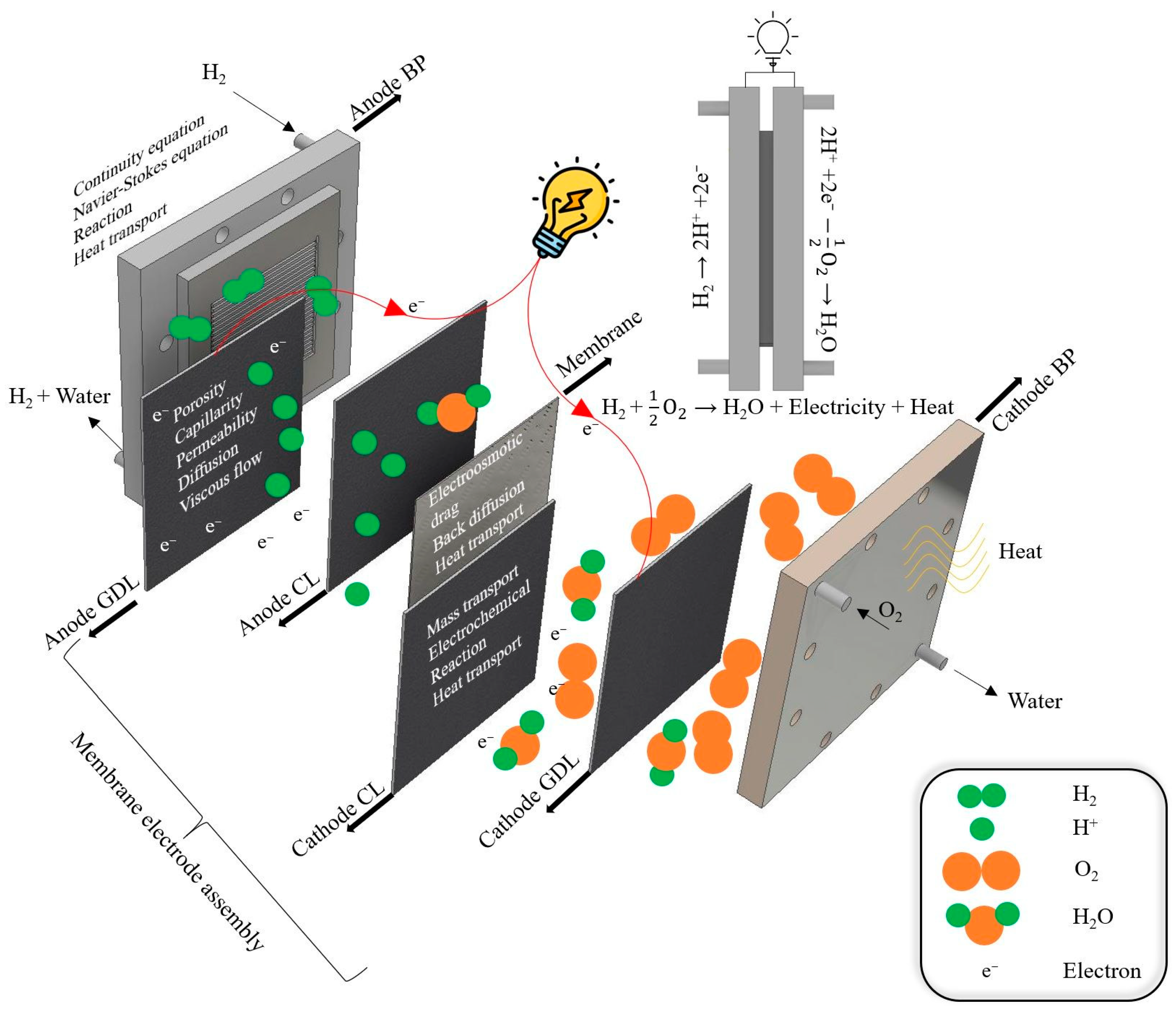
4. PEMFC Fundamentals and Modeling Consideration of Components with ML

PEMFCs are devices that convert chemical energy into electrical energy. They consist of a membrane electrode assembly (MEA) and bipolar plates (BPs) on both sides, as shown in Figure 1.

The MEA consists of a membrane sandwiched between an anode (negatively charged) and a cathode (positively charged) catalyst layer (CL), followed by a gas diffusion layer (GDL). On the anode side, hydrogen enters as a fuel and is oxidized into a proton (H⁺) after hydrogen oxidation reaction (HOR) occurs (Equation (1)), whereas on the cathode side, the oxygen reduction reaction (ORR) happens (Equation (2)). A potential difference is formed between the sides owing to the flow of electrons, and water is generated as a byproduct on the cathode side (Equation (3)). The electrochemical reactions are as follows [8,28]:

Anode side: H₂ → 2H⁺ +2e⁻

(1)

$$\mathrm{Cathode}\mathrm{side}:2{\mathrm{H}}^{+}+2{\mathrm{e}}^{-}-\frac{1}{2}{\mathrm{O}}_2\to {\mathrm{H}}_2\mathrm{O}$$

(2)

$$\mathrm{Overall}\mathrm{reaction}:{\mathrm{H}}_2+\frac{1}{2}{\mathrm{O}}_2\to {\mathrm{H}}_2\mathrm{O}+\mathrm{Electricity}+\mathrm{Waste}\mathrm{heat}$$

(3)

Table 3. Functions and materials used for PEMFC components.

Components	Functions	Materials (Present)	Materials (Future)	Reference
Polymer electrolyte Membrane	-Conduction of protons -Separating barriers of reactants. -Blockade of electrons.	-Perfluorosulfonic acid (PFSA) membranes (~90 °C operations).	-Composite membranes such as Polytetrafluoroethylene (PTFE) and Polyvinylidene difluoride (PDDF) membranes (>100 °C operations). -PEM with ionogels	[23,76,77]
Catalyst layer	Site of electrochemical reactions.	-Platinum (Pt) loading (0.1–0.2 g kW−1). -Heterogenous coverage of ionomer.	-Platinum (Pt) loading (<0.1 g kW−1). -Lower and better distribution of ionomer. -Pt monolayer catalysts, nanometer film catalysts, controlled crystal shape catalysts, and non-PGM catalysts.	[23,76]
Gas diffusion layer	-Distribution of reactants. -Water management. -Electricity and heat distribution through conduction.	-Carbon paper with fiber structure -Carbon black and hydrophobic agents	-Carbon paper with modified fiber configurations. -Carbon black with super hydrophobic additives. -Metal foam.	[23,76]
Bi-Polar plate	-Transport of reactants. -Water management. -Dissipation of heat. -Current collector.	-Graphite (~1 mm thick). -Metal (~0.6 mm thick).	-Metal foam. -Metal (~0.5 mm thick).	[23,76]

shows the functions of each component, state of the art, and future trends.

4.1. Modeling of Polymer Electrolyte Membrane

The PEM is one of the key components of the PEMFC. It enables protons (H⁺) to move from the anode to the cathode to react with O₂ and produce water. An ideal membrane should possess high proton conductivity at low humidity, good chemical and mechanical stability, low electronic conductivity, low water permeability, and impermeability to reactants [78,79]. Moreover, manufacturing it should be easy and economical. The most commonly used membrane is Nafion, which is composed of perfluorosulfonic acid (PFSA). Membrane modeling is generally classified into two approaches: microscopic and macroscopic.

4.1.1. Microscopic

To understand the effect of ionic moieties [80], which are responsible for making the membrane more soluble in water despite being made of hydrophobic polymers, and the backbone dynamics [81,82] of Nafion as well as the oxygen permeation [83], conduction, and mobility of protons, various approaches such as statistical [84] and molecular dynamic (MD) simulations [85] have been used. Harvey et al. [84] proposed a one-dimensional (1D) MEA performance model, which includes liquid water transportation, an agglomerate catalyst structure, and various statistical MEA characteristic parameters. This model provided insights into the effect of Pt loading near the interface between the CL and membrane on the reaction distribution. Figure 2a shows the experimental validation of the statistical simulation model, and Figure 2b depicts the partial effect of high liquid water on a low oxygen partial pressure when the Pt loading is low. Kwon et al. [85] performed MD simulations to measure the solubility and permeability of O₂ in saturated PFSA ionomers on a Pt surface using two types of PFSA ionomers by varying the water content.

Their simulation results provided guidance for designing better PFSA ionomers for PMFCs. Figure 2c presents an equilibrated structure where Nafion ionomers with high water content and water molecules are denser in the region of saturated Nafion–Pt interfaces because of their strong attraction. Additionally, dissolved O₂ molecules have the highest density, whereas water molecules (hydronium ions) have the lowest inside the hydrated Nafion.

Table 4. Microscopic research of PEMFC membrane.

Research Method	Software/Code	Findings	Reference
MD simulation	Materials studio (MS) 4.3 COMPASS	Instead of Nafion, most widely used membrane material, a natural polymer Chitosan (a derivative of chitin a natural polysaccharide found in insects, fungi, and yeast) was used. The highest conductivity of 7.14 × 10−2 S/cm was observed when the system contained 40% of water.	[86]
MD simulation	Materials studio (MS) 4.4 COMPASS	The diffusion of water molecules and hydronium ions in Nafion 117 are measured using MD simulation. They found that the diffusion coefficient of both water molecules and hydrogen ions increase with the water content when the temperature in constant. Similar to this, both the diffusion coefficient increases with the temperature at constant water content.	[87]
MD simulation	COMPASS	Proton conductivity of three different types of polymer membrane; Dow, Nafion and Aciplex was compared. The Aciplex membrane has the optimum proton mobility and best water molecules and hydronium mobility at 350 K.	[88]
MD simulation	Materials Studio COMPASS II	Sulfonated polynorbornene-based (SPNB) membranes swell upon after getting hydrated and divided into hydrophobic and hydrophilic regions having sulfonic acid groups at their interfaces. Also, more water molecules can absorb the sulfur atoms and hydronium due to the rise of water at increasing temperature.	[89]
MD simulation	LAMPPS	Pt/C models were investigated with various PTFE-binder content in the presence of H3PO4 at 298.15 K and 433.15 K. It was found that the coverage of H3PO4 is higher at high temperature in comparison to lower temperature as the H3PO4 could still manage to contact the Pt surface through PTFE-binder due to favorable interactions.	[90]

lists some microscopic-level research methods and their results.

Despite the importance of the results of microscopic models, integrating them into a complete fuel cell model is difficult, which leads to the separation of the microscopic model research. However, one particular membrane property, that is, the water content (the number of H₂O moles per mole of sulfonic acid group), can be utilized in macroscopic models because it influences the membrane structure.

4.1.2. Macroscopic

When modeling a membrane from a macroscopic perspective, two models are commonly used: sorption and transport.

Sorption Model

In PEMFCs, the membrane material adsorbs water when the environment is humid. The water content, λ, is defined as the number of water molecules per mole of sulfonic acid and is expressed as follows [91]:

$$\lambda \equiv \frac{n\left(H_{2}O\right)}{n\left(S{O}_3\right)}$$

(4)

The water content could be equivalently expressed as a function of total mass of water ($m_w$) within the same reference volume (V) [92]:

$$\lambda =\frac{m_w}{M_w{c}_{f}V}$$

(5)

Again, sorption of water is the measurement of the amount of water adsorbed by the membrane when the membrane is in equilibrium with water vapor/liquid at a given temperature. This term is known as the sorption isotherm, and it relates to the equilibrium water content ${\lambda }_{eq}$, which is the function of water activity $a_w$ in the membrane phase [92]:

$${\lambda }_{eq}={\lambda }_{eq}\left(a_w\right)$$

(6)

Water could be in a position where it sorbed from or desorbed to a nearby phase. These conditions are referred to as vapor-equilibrated (VE), where a gas phase reacts with water vapor at a certain water activity, and liquid-equilibrated (LE), a liquid phase. Both saturated water vapor and pure liquid water are treated as same, as they equally processed the same $a_w=1,$ generates a thermodynamically unexpected scenario often known as “Schröder’s paradox” [93]. Though some of the experiments did not observe this [94,95], research suggests VE water contents are closer to a typical LE value, suggesting the presence of thin water film.

In the membrane, the activity of water can be expressed as the activity of water vapor in the equilibrating gas phase under VE conditions [91]:

$$a_w=a_{w,vap}\left(equilibrium\right)$$

(7)

However, the $a_w$ in the vapor phase can be approximated from the ration between the partial pressure of water, $p_{w,vap}$ and the saturated partial pressure of water, $p_{sat}\left(T\right)$ as a function of temperature (T) [92]:

$$a_{w,vap}\approx \frac{p_{w,vap}}{p_{sat}\left(T\right)}\equiv \frac{x_{w}p}{p_{sat}}$$

(8)

where partial pressure of water is the function of mole fraction of water vapor, $x_w$ and p is the pressure of the gas mixture in the pore region.

The above equation ignores the fugacity correction considering the operating condition of PEMFC is close to the absolute pressure [92]. The saturated vapor pressure $P_{sat}$ can be expressed as the following empirical equation [96]:

$${\log }_{10}\left(\frac{p_{sat}}{p_0}\right)=a_0+a_1\left(T-T_0\right)+a_2{(T-T_0)}^2+a_3{(T-T_0)}^3$$

(9)

Table 5. Variations of water content, λ.

Equation	Remarks	Ref.
$\lambda =\left\{\begin{array}{cc}1.41+11.3a_w-18.8a_w^2+16.2a_w^3\hfill & 0\le a_w\le 1\hfill \\ 10.1+2.94\left(a_w-1\right)\hfill & 0<a_w\le 3\hfill \\ \hspace{1em}16.0\hfill & 3<a_w\hfill \end{array}\right.$	This equation is obtained from the fitting experimental data of water uptake in Nafion membrane at 80 °C	[97]
$\lambda =\left\{\begin{array}{c}0.3+6a_w[1-\tanh (a_w-0.5)]+3.9\sqrt{a_w}[1+\tanh (\frac{a_w-0.89}{0.23})]\\ \hspace{1em}\hspace{1em}\hspace{1em}\hspace{1em}\hspace{1em}\hspace{1em}\hspace{1em}\hspace{1em}\hspace{1em}s\le 0\\ 16.8s+{\lambda }_{\left|\left(a=1\right)\right.}\left(1-s\right)\hspace{1em}\hspace{1em}s>0\end{array}\right.$		[98,99]
$\lambda =\left\{\begin{array}{cc}0.043+17.18a_w-39.85a_w^2+{36a}_w^3\hfill & {0\le a}_w\le 1\hfill \\ 14+1.4\left(a_w-1\right)\hfill & 1\le a_w\le 3\hfill \end{array}\right.$	Although the relation in $a_w$ > 1 obtained from 80 °C, the polynomial relation comes at 30 °C	[96]
$\lambda =1.4089+11.26a_w-18.768a_w^2+16.209a_w^3\hspace{1em}0\le a_w\le 1$	A fit data obtained from the experiment under VE conditions at 80 °C	[100]

contains the water contain measurement equation at various conditions.

Transport Models

The macroscopic transport models are mainly distinguished into three approaches depending on the driving forces: (1) Chemical potential, (2) diffusion, and (3) hydraulic models.

Diffusive Model

This model considers the membrane as a system of single and homogeneous phases where protons and water move and dissolve by the diffusion process. Though both water and protons can be moved in a stationary membrane system, water movement is neglected or treated as constant for the sake of simplicity. Thus, the differential form of Ohms law is implemented for defining proton movement [97]:

$$i_2=-\kappa \nabla {\mathsf{\Phi }}_2$$

(10)

where $\kappa$ is the ionic conductivity of the membrane, ${\mathsf{\Phi }}_2$ is the chemical potential of the membrane. This model can be described using the dilute solution theory proposed by Newman [101]. This theory is evaluated only by the dilute concentration theory (DCT), which treats ionomers as solvents and water and protons as solute species. Assuming the negligible effect between the water and proton (most solute species are dilute in water), DCT implements the following Nernst–Planck equation to measure the interaction between the solute species and ionomer [101]:

$$\underset{\mathrm{Flux}}{\underbrace{N_i}}=\underset{\mathrm{m}\mathrm{i}\mathrm{g}\mathrm{r}\mathrm{a}\mathrm{t}\mathrm{i}\mathrm{o}\mathrm{n}}{\underbrace{-z_i{u}_{i}F{c}_i\nabla {\mathsf{\Phi }}_2}}-\underset{\mathrm{d}\mathrm{i}\mathrm{f}\mathrm{f}\mathrm{u}\mathrm{s}\mathrm{i}\mathrm{o}\mathrm{n}}{\underbrace{D_i\nabla c_i}}+\underset{\mathrm{c}\mathrm{o}\mathrm{n}\mathrm{v}\mathrm{e}\mathrm{c}\mathrm{t}\mathrm{i}\mathrm{o}\mathrm{n}}{\underbrace{c_i{v}_2}}$$

(11)

The migration term (1st part of the equation), containing the information of motion of charged species, related to potential gradient ($-\nabla {\mathsf{\Phi }}_2$) and charged number, $z_i$, Faraday’s constant, F, (9.6487 × 10⁷ C/kmol) concentration, $c_i$ and mobility, $u_i$. The midterm (diffusion) is composed of a concentration gradient, $\nabla c_i$ and a diffusion coefficient, $D_i$ which is the function of mobility, $u_i$ and can be expressed by the Nernst–Einstein equation [101,102,103]:

$$D_i=RT{u}_i$$

(12)

The convective term (final part of the equation) is the function of the concentration and motion of the solvent. However, this term will become null for the analysis of a single-phase system. The migration term of Equation (11) becomes zero as the water has a zero valence and is converted to Fick’s law [104].

$$N_w=n_d\frac{i_2}{F}-D_w\nabla c_w$$

(13)

where $\xi$ is the electroosmotic drag coefficient.

Chemical Potential Model

In this model, though the main force of transport is chemical potential, diffusion (gradients of species concentration) and convection (gradient of pressure) are also included. Based on the concentrated solute theory proposed by Bennion [105,106], three independent transport properties should be considered:

• Chemical potential of proton, Φ₂
• Transport coefficient of water, α_w
• Chemical potential of water, μ_w

The final equation containing these transport systems is as follows [105]:

$$i_2=-\frac{\kappa n_d}{F}\nabla {\mu }_w-\kappa \nabla {\mathsf{\Phi }}_2$$

(14)

$$N_w=n_d\frac{i_2}{F}-{\alpha }_w\nabla {\mu }_w$$

(15)

In addition to the above equations, the irreversible thermodynamics approach [107,108], generalized Stefan–Maxwell equations [109,110,111,112], and dusty fluid model [113,114,115] are also used. Unlike the diffusion model, proton–water interaction is considered in this model. Though this interaction is very rare, it should be considered in situations where the gradient of water is very high, such as low humidity or high current density conditions. It should be noted that Equations (12) and (14) are similar except that the concentration and diffusion coefficient of water have been replaced by the chemical potential and transport coefficient of water, respectively. However, the chemical potential model is not well recognized for modeling PEMFC because of the difficulties in obtaining the transport parameters.

Hydraulic Model

This model treats the membrane as a two-phase system, unlike the diffusive and chemical potential models. Also, the addition of a second phase facilitates the hydraulic model to consider the pressure gradient responsible for the convective in the water. However, the water content of the membrane is assumed to remain constant (λ = 22) [116] as long as the water contains the pores to assist convective transportation. Bernardi et al. [117,118] proposed this model based on previous works [119,120,121], where a dilute solution approach with Equation (10) (Nernst–Planck equation) is used to characterize the movement of proton, and instead of zero, the velocity of the water is given by Schlogl’s equation [122]:

$$v_w=-\left(\frac{k}{\mu }\right)\nabla p_L-\left(\frac{k_{\mathsf{\Phi }}}{\mu }\right)z_f{c}_{f}F\nabla {\mathsf{\Phi }}_2$$

(16)

where $k$, $k_{\mathsf{\Phi }}$, $p_L$, $\mu$, and $z_f{c}_f$ are the effective hydraulic permeability, effective electrokinetic permeability, liquid pressure, water viscosity, charge and concentration of fixed ionic sites, respectively.

This model also assumes a constant gas volume fraction in the membrane, though it does not represent the real experiment. This assumption (constant gas volume fraction) allows the gas to crossover through the membrane. However, the anode side near the membrane quickly dried out most of the time due to the vigorous EOD effect during PEMFC operation, which contradicts the assumption of a fully hydrated membrane. Thus, this model suffers from an unrealistic scenario by neglecting diffusive water transport [123].

Also, the concentration solution approach could be utilized in this model as previously conducted by Weber and Newman [124], where the same Equations (14) and (15) are used except the chemical potential is replaced by liquid pressure and the transport coefficient is changed to permeability through comparison of Darcy’s law.

Hence, Equation (15) transforms [124]:

$$N_w=n_d\frac{i_2}{F}-\frac{k}{\mu {\overline{V}}_w}\nabla p_L$$

(17)

Here, ${\overline{V}}_w$ is the molar volume of water.

Combination Model

In order to portray the real experimental condition, diffusive and hydraulic models should be utilized together to cancel out the limitations of each model. A modeling of differentially pressurized PEMFC should consider both diffusive and convective water transport by adding diffusive, convective, and EOD terms, which result in a combination of diffusive and hydraulic models [114,125,126,127,128]. Hence, the new equation becomes [114]:

$$N_w=n_d\frac{i_2}{F}-\frac{k}{\mu }\nabla p_G-D_w\nabla c_w$$

(18)

4.1.3. Combined Model (Microscopic and Macroscopic)

Only one component of the microscopic model, namely the water content λ, can be successfully integrated into the macroscopic model [100]. Water is absorbed by the dry membrane to solvate the acid groups, and as the water content increases, the water droplets agglomerate and form interconnecting channels. Figure 3 displays the changes in the membrane structure depending on the water content, where the gray, black, and light gray areas represent the fluorocarbon matrix, polymer side chain, and liquid water, respectively, whereas the dotted line denotes the collapsed channel. When the amount of water exceeds the percolation threshold (λ = 2), a complete cluster channel is formed, as illustrated in Figure 3c. The formation of water channels indicates whether the water at the boundary is in the vapor (Figure 3c) or liquid (Figure 3d) state, termed VE or LE membranes, respectively. In the VE case, the channels are not well connected, whereas in the LE case, they are filled with water, expanded, and connected. These two distinctive structures form the foundation of the two macroscopic models: diffusive and hydraulic.

4.1.4. Issues Related to State-of-Art Membrane Modeling

When it comes to water transport, the chemical potential model remains the most comprehensive solution among the membrane modeling approaches. However, a combined diffusive and hydraulic model with the addition of EOD remains a better choice because it considers most of the aspects of experimental findings [116]. Regardless of various options, current membrane modeling has the following issues:

Despite the technological advancement of membrane materials, the majority of research papers on the numerical investigation of PEMFC still rely on the springer model [96] and the Weber–Newmann model [124], which are based on experimental work [96,129,130,131], dating back to 1998 [92].

Electroosmotic drag (EOD) could have a different value depending on the electrodes (anode and cathode) [132]. As a result, the standard practice is to consider EOD as a source term on the cathode side and a sink term on the anode side, according to previous research [132,133].

Even though the EOD increases with the water content, λ based on a number of correlations observed from the experiment [96,134,135,136] as mentioned in Table 3, the differences among them introduce certain uncertainties during modeling [35].

Due to small pressure imbalances and low membrane permeability, the effect of cross-diffusion of reactants through the membrane is usually neglected [35], which is not true in some cases. The results indicate that this effect is not always insignificant, particularly when calculating cell efficiency. In some instances, the cross-over effect has been observed to impact cell efficiency by approximately 2% [137].

The recent introduction of reinforced membrane (typical thickness of 25–35 μm) in PEMFC helps to mitigate membrane degradation by reducing resistance and improving water management without compromising mechanical strength [138]. However, the composite nature of this type of membrane and the effect of its conductivity, diffusivity, water intake, and mechanical coupling in MEA to transport phenomena are not well understood [92].

Previous research [139,140] found that the convection type of transport, by considering the microporous membrane and its percolation phenomena, could give the membrane resistance close to the experimental value in comparison to the model that utilizes diffusion transport. However, convection models are not widely used due to their underestimation of dehydration.

Modeling approaches are still not considering the effect of free radical scavengers [141] or different additives [142] to alleviate the chemical degradation of modern membranes.

The effect of mechanical and chemical degradation [143] of membranes on the performance of PEMFC was not considered in the modeling.

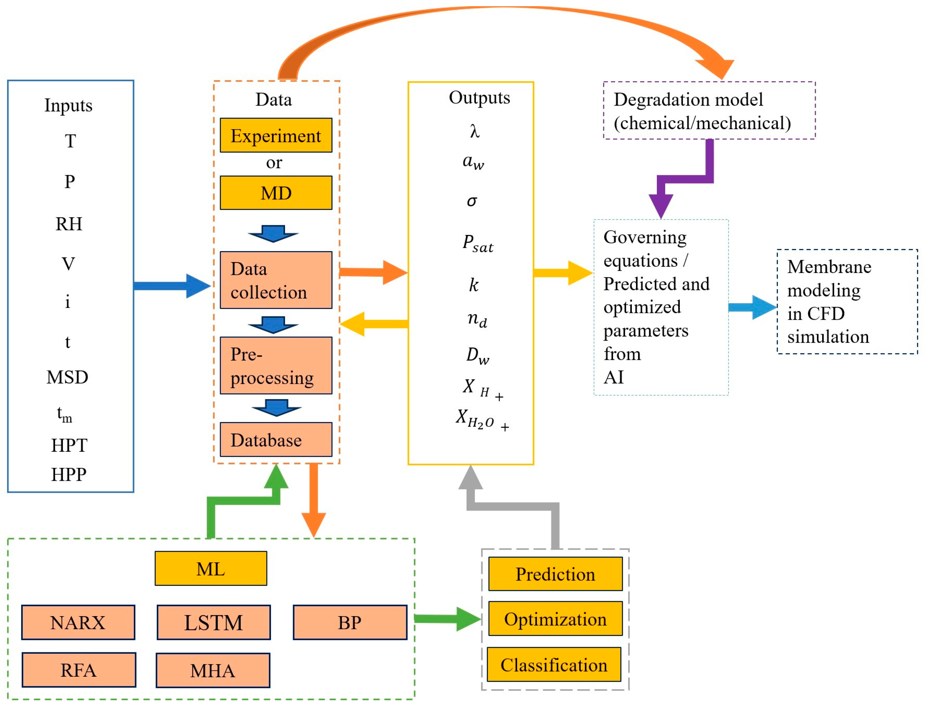
4.1.5. ML in the Field of Membrane

Previous researchers are trying to use ML to design and optimize membranes [44,144,145,146,147,148,149,150,151], predict membrane properties [36,43,152], diagnose membrane conditions [153,154], and prevent membrane degradation [155,156,157]. Cho et al. [43] collected data from a 1.2 kW PEMFC in a MATLAB/Simulink environment and used that data to train a nonlinear autoregressive network (NARX) with Bayesian optimization to predict the voltage, temperature, and membrane water content (Max. error of MSE 2.14 × 10⁻⁴). Figure 4a shows the architecture of the proposed NARX network. Huo et al. [154] utilized a genetic algorithm-based back propagation (GA-BP) neural network to predict membrane hydration in PEMFC. A dynamic model of PEMFC was used, which contains cathode mass flow, anode mass flow, membrane water content, and a stack voltage sub-model. Figure 4b depicts the GA-BP neural network, showing a better prediction of hydration in comparison to a least-squares support vector machine (LS-SVM) regarding mean square error (MSE), mean absolute error (MAE), and root mean square error (RMSE). In order to reduce the extensive work, resources, and time, Huo et al. [145] proposed a random forest feature selection process to identify the important features as input parameters, as verified by the previous studies. Subsequently, a convolutional neural network (CNN) with batch normalization and dropout methods is implemented to predict the performance of PEMFC, such as the I–V curve, as can be seen in Figure 4c. It is important to note that, among the important factors, the membrane contains hot press time (HPT), hot press pressure (HPP), hot press temperature (HPT), which is required for manufacturing, MEA, and the thickness of the membrane. Gu et al. [155] established a long short-term memory (LSTM) network model to diagnose the flooding fault of a bench test of a 92 kW vehicle with a fuel cell system, which is essential for the identification of membrane hydration conditions. Once the LSTM diagnosis network was built, it could effectively predict the condition of fuel cells instead of relying on a large number of sensors, which can effectively reduce the cost of an efficient system. Figure 4d shows the input parameters of the LSTM network and the results of the network in comparison to the diagnosis from actual THDA (total harmonic distortion analysis) diagnostic equipment.

4.1.6. Integration of ML in Membrane Modeling

A potential integration of ML and CFD modeling is shown in Figure 5. For membrane modeling, a large number of datasets could be obtained from experiments and MD simulations. That includes boundary conditions from the real test, such as temperature, pressure, RH, etc.; water content from the MD simulation; and variables such as temperature, pressure, and time to manufacture MEA by the hot pressing method [158] as input. In addition to that, the ML method was used to optimize the input parameters and predict the corresponding output parameters by considering the degradation of membrane properties. Finally, the governing equations are modified depending on the change in properties due to more precise input parameters, the change in output due to material degradation, and membrane modeling.

4.2. Modeling of Catalyst Layer (CL)

The CL is the location where the HOR and ORR occur (Equations (1) and (2)). It is often the thinnest component [159] (5 to 30 μm) in the PEMFC because of its high material cost, yet it handles the most complex transport phenomena [160]. Usually, fine particles of Pt and its alloys are sprayed on high-surface-area carbon in the active porous layer of the electrode to minimize Pt loading (0.1–0.4 mg·cm⁻²) [161]. For effective usage, the CL must be positioned to form a triple-phase reaction interface at the intersection of e⁻, H⁺, and reactive gas transfer channels. The different CL models are as follows: interface, microscopic, single pore, and simple macrohomogeneous.

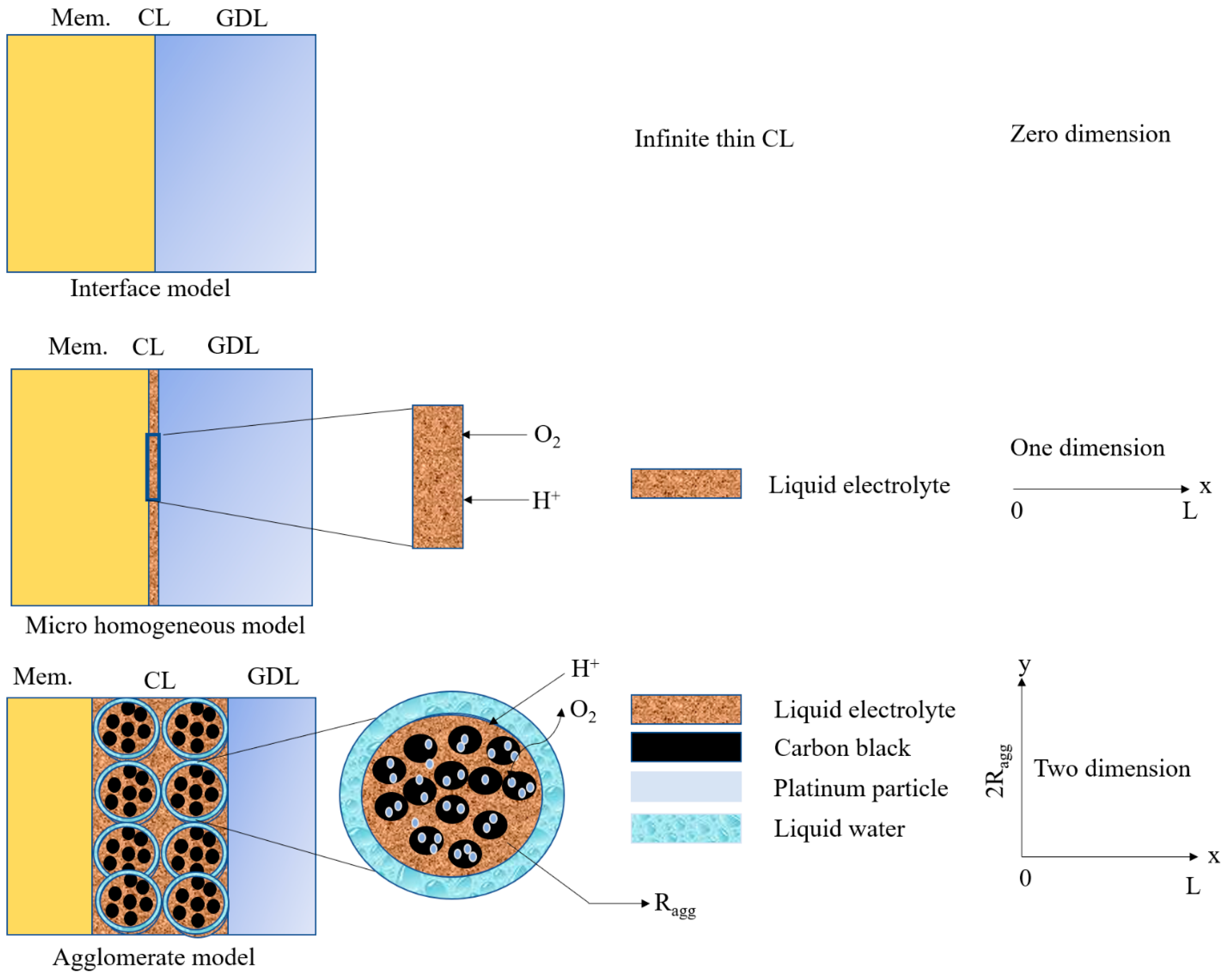
4.2.1. Interface Model

Among the CL models, the simplest model treats the CL as an interface between the GDL and membrane. For this purpose, the CL is assumed to be an infinitely thin layer, and its physical structure is completely ignored. Although computationally economical and efficient, this model is not appropriate when the main focus is on the CL [116]. Therefore, the CL can be considered the location where H₂ and O₂ are consumed and water is produced. The generation and consumption terms are expressed using Faraday’s law [116]:

$$N_{i,k}={\displaystyle \sum _h}{S}_{i,k,h}\frac{i_{h,1-k}}{n_{h}F}$$

(19)

Here, $S_{i,k,h}$ is the stoichiometric coefficient of species i in phase k; $i_{h,1-k}$ is the normal interfacial current transferred per unit interfacial area across the interface between the electronically conducting phase and phase k owing to the electron-transfer reaction h, and it is positive in the anodic direction.

For the aforementioned model, detailed information on the potential is not essential. In previous research [99,162,163,164] on water management, a similar technique was used by quantifying it with the current density. Both the resultant water on the cathode side and the electroosmotically dragged water are proportional to the current density [162]. In addition to Equation (19), researchers [125,165,166,167,168] have utilized a slightly more sophisticated approach by fitting a polarization curve to a single expression as follows [125]:

$$E=U^{\prime }-R^{\prime }i-\frac{RT}{{\alpha }_{c}F}\ln \left(i\right)+\frac{RT}{{\alpha }_{c}F}\ln (1-\frac{i}{i_{lim}})$$

(20)

where E is the cell potential and i is the superficial current density through the MEA, whereas ${\alpha }_c$ is the cathodic transfer coefficient.

To obtain a more sophisticated interface model, reaction kinetics such as the Tafel equation have been incorporated [169,170] with the Butler–Volmer equation [171,172,173], which can be expressed as:

$$i_{h,k-p}=i_{0_h}\left[{\displaystyle \prod _i^a}\frac{p_i}{p_i^{ref}}{exp}^{\left(\frac{{\alpha }_{a}F}{RT}\left({\mathsf{\Phi }}_k-{\mathsf{\Phi }}_p-U_h^{ref}\right)\right)}-{\displaystyle \prod _i^c}\frac{p_i}{p_i^{ref}}{exp}^{\left(\frac{{-\alpha }_{c}F}{RT}\left({\mathsf{\Phi }}_k-{\mathsf{\Phi }}_p-U_h^{ref}\right)\right)}\right]$$

(21)

New models have utilized a kinetic expression that considers multidimensional aspects, which is an improvement over the previous model (Equation (10)). However, this model (Equation (21)) is based on the assumption that the surface overpotential and concentration of reactant gases are uniform in the CL, and it uses the overpotential of the kinetic expression as a fitting parameter. Despite its simplicity and efficient calculation, this model is still limited because it does not consider multiple aspects of the CL that are not actually uniform. This model is not suitable for optimizing CL fabrication in terms of the effects of Pt loading, compressive load, and pore size.

4.2.2. Microscopic and Single Pore Models

Most of the earliest CL models were microscopic and single-pore models that were easily solvable. These models were utilized for the CL of phosphoric acid fuel cells with Teflon-coated pores for gas diffusion, whereas the rest of the area was flooded with a liquid electrolyte. Although a detailed microstructure is required for this model, effective values such as diffusivity and conductivity are not required because they are assumed to be homogeneous throughout the microstructure. Single-pore models are divided into two types according to their nature.

In the first model, known as the gas pore model, the pores are considered straight and cylindrical with a specific radius [174,175,176,177]. In addition, these pores extend to the length of the CL, and reactions occur on the surface.

Among the single-pore models, the flooded agglomerate model shows potential for real experimental data. This model still uses gas pores, although some of them are filled with electrolyte and catalyst [178,179,180,181,182,183]. In those filled pores, reactions, diffusion, and migration occur. Consequently, this model works better than the gas pore model because it covers a larger area.

However, pores with different porosities and tortuosities exist in real cases, and the electrolyte in PEMFCs is solid, unlike in phosphoric acid fuel cells, which are not supposed to penetrate the pores. Although the single-pore model is adequate, it is not suitable for simulating the CL in detail.

In addition to the two aforementioned models, a spherical agglomerate model, which considers special agglomerate structures in three-dimensional (3D) hexagonal arrays, was introduced by Antoine et al. [184]. Among the agglomerates, either gas pores or regions are flooded with electrolyte [185,186]. This model examines the interactions that depend on the placement of these agglomerates. In addition to Ohm’s and Fick’s laws, the reaction kinetic equation can be solved by employing this model.

The concentration contours around the electrocatalyst particles and can be validated by experimental current density trends. In contrast to the interface model, this model can depict the occurrence of HOR near the membrane and the effect of the packing and structure of agglomerate particles on the overall efficiency of the CL.

4.2.3. Simple Macrohomogeneous Model

Introduced initially by Tiedemann and Newman [187], the macrohomogeneous model neglects exact geometric details by treating the CL structure as a randomly arranged porous domain. Only a few variables, such as porosity, volume fraction, and surface area per volume, are used to represent the structure of the CL. Moreover, the transport properties should be averaged over the CL volume. Although this model does not include the detailed structure of the domain, it shares many similar theoretical expressions with the single-pore model. Two of the main length scales of this model are explained here [116].

Porous Electrode Model

Although it is based on the assumption of a single-pore model, the porous electrode model calculates the overall reaction without considering the detailed structure of the computational domain. In this model, the concentration and potential are assumed to be uniformly distributed in the agglomerates, indicating that the main interaction does not affect the agglomerates. The equations governing the simple porous electrode models are listed in

Table 6. Important variables and governing equations for the CL [116].

Variable	Porous Electrode Model	Agglomerate Model
Overall liquid water flux, NL	$$\begin{gathered} \frac{\partial {ϵ}_k{c}_{i,k}}{\partial t}=-\nabla ·N_{i,k}-{\displaystyle \sum _h}{a}_{l,k}{s}_{i,k,h}\frac{i_{h,1-k}}{n_{h}F} \\ \hspace{1em}\hspace{1em}\hspace{1em}\hspace{1em}\hspace{1em}\hspace{1em}\hspace{1em}+{\displaystyle \sum _I}{S}_{i,k,l}{\displaystyle \sum _{p\ne k}}{a}_{k,p}{r}_{i,k-p} \\ \hspace{1em}\hspace{1em}\hspace{1em}\hspace{1em}\hspace{1em}\hspace{1em}\hspace{1em}+{\displaystyle \sum _g}{s}_{i,k,g}{ϵ}_k{R}_{g,k} \end{gathered}$$
Overall membrane water flux, NW	Equation above.
Gas-phase component flux, NG,i	Equation above.
Gas-phase component partial pressure, pG,i	$\nabla x_i=-\frac{N_i}{c_T{D}_{K_i}^{eff}}+{\displaystyle \sum _{j\ne i}}\frac{x_i{N}_j-x_j{N}_i}{c_T{D}_{i,j}^{eff}}$
Liquid pressure, pL	$$\begin{gathered} N_{w,L}=-\frac{k}{{\overline{V}}_w\mu }\nabla p_L=-\frac{k}{{\overline{V}}_w\mu }\left({\nabla p}_c+{\nabla p}_G\right)= \\ \hspace{1em}\hspace{1em}\hspace{1em}\hspace{1em}\hspace{1em}-\frac{k}{{\overline{V}}_w\mu }\nabla p_c \end{gathered}$$
Membrane water chemical potential, μw	Equation (14)/Equation (16)
Electronic-phase current density, i1	$i_1=-{\sigma }_0{ϵ}_1^{1.5}\nabla {\mathsf{\Phi }}_1$
Membrane current density, i2	Equation (9)/Equation (13)
Electronic-phase potential, Φ1	${\displaystyle \sum _k}\nabla ·i_k=0$
Membrane potential, ΦL	$i_s=-{\kappa }_s^{eff}\nabla {\varphi }_s$	$$\begin{gathered} \nabla ·i_s=4F\frac{P_{O_2}}{H}{\left(\frac{1}{E_r{k}_c\left(1-{\epsilon }_{cat}\right)} \\ \hspace{1em}\hspace{1em}\hspace{1em}\hspace{1em}\hspace{1em}+\frac{\left(r_{agg}+\delta \right)\delta }{a_{agg}{r}_{agg}D}\right)}^{-1} \end{gathered}$$ Where $E_r=\frac{1}{{\mathsf{\Phi }}_L}\left(\frac{1}{\tanh \left(3{\mathsf{\Phi }}_L\right)}-\frac{1}{3{\mathsf{\Phi }}_L}\right)$
Temperature, T	$$\begin{gathered} {\displaystyle \sum _k}{\rho }_k{\widehat{C}}_{P_k}\left(\frac{\partial T}{\partial t}+v_k·\nabla \mathrm{T}\right) \\ \hspace{1em}\hspace{1em}\hspace{1em}\hspace{1em}\hspace{1em}={\displaystyle \sum _k}{h}_{k,ext}{a}_{k,ext}\left(T_{ext}-T\right) \\ \hspace{1em}\hspace{1em}\hspace{1em}\hspace{1em}\hspace{1em}+\nabla ·\left(k_T^{eff}\nabla T\right) \\ \hspace{1em}\hspace{1em}\hspace{1em}\hspace{1em}\hspace{1em}-{\displaystyle \sum _k}{\displaystyle \sum _i}{J}_{i,k}·\nabla {\overline{H}}_{i,k} \\ \hspace{1em}\hspace{1em}\hspace{1em}\hspace{1em}\hspace{1em}+{\displaystyle \sum _{1-k}}{\displaystyle \sum _h}{a}_{1,k}{i}_{h,1-k}\left({\eta }_{s_{ORR,1-k}} \\ \hspace{1em}\hspace{1em}\hspace{1em}\hspace{1em}\hspace{1em}+{\displaystyle {\mathsf{\Pi }}_h}\right)+∆H_{evap}{r}_{evap} \end{gathered}$$ Or $Q={\displaystyle \sum _{k-p}}{\displaystyle \sum _h}{a}_{k,p}{i}_{h,k-p}\left(U_{H_h}-V\right)$
Total gas pressure, pG	$v_G=-\frac{k_G}{{\mu }_G}\nabla p_G$
Liquid saturation, S	${\epsilon }_G={\epsilon }_0\left(1-S\right)$

. Although the thickness of the CLs serves as the characteristic length scale, there are some variations in the treatment of the simple porous electrode model.

In the first variation, the CLs are integrated and included as boundary conditions when calculating the cell potential or current density [128,188,189]. This treatment is similar to that of the interface models, except that it considers potential drops for the matrix and solution phases. The rationale for the integration is that it does not result in a loss of numerical accuracy and provides numerical stability and easier convergence, particularly when the reaction distribution is mainly uniform.

The second variation uses a simple porous electrode modeling approach, considering a CL of finite thickness and using the equation in Table 6. Although most of these models allow the diffusion mass transfer of reactant gases [112,118,190,191,192], in some previous studies, the concentration of the reactant gases has been assumed to be uniform throughout the CL [193,194,195]. In the final variation of the porous electrode model, rather than gas diffusion in the CL, the reactant gases are assumed to be dissolved in the electrolyte and transported by diffusion and reaction [196,197,198,199]. This model is closer to the thin film model, which does not consider gas pores [200,201]. The governing equations in Table 6 are well suited for solving this model, except that a concentration term should be added to the kinetic expressions instead of the partial pressure. Accordingly, a mass transport equation for the reactant or product gas should be added to account for diffusion effects on the membrane or water.

Agglomerate Model

This model considers the radius of the agglomerate as a characteristic length scale in addition to the CL thickness. Most of these agglomerates are assumed to be either large spheres, a combination of Nafion, carbon, and Pt particles [202,203,204], or small spheres, a void consisting of carbon and Pt particles filled with liquid water [205,206]. In the simple homogeneous agglomerate model, the main effects are assumed to occur at the agglomerate length scale. Hence, the reaction rate distribution, that is, gas concentration and surface overpotential, is uniform throughout the thickness of the CL. It is assumed that oxygen diffuses through the gas pores, dissolves into agglomerates through the electrolyte/water, and then reaches the reaction site by diffusion again. The mathematical expressions are similar to those of the microhomogeneous model indicated in Table 4, except that spherical and cylindrical coordinates are added for the gradients. Another agglomerate model, known as the embedded macrohomogeneous model, considers both the aforementioned macrohomogeneous model and reaction and overpotential distribution in the agglomerates that are disregarded in the simple homogeneous agglomerate model. These effects are essential when CL hydration and dehydration are considered. Figure 6 shows the distinctive features of the three catalyst models.

In addition to the equations presented in Table 6, in this model, either a mass transfer term [207,208,209] (1st approach) or an effectiveness factor incorporating the agglomerate equation [210,211,212] (2nd approach) is used. Previous studies have reported that the agglomerate model is better than the macrohomogeneous model because it uses more empirically controlled parameters [204,213]. In particular, at higher current densities, the agglomerate model can predict the voltage drop, unlike the macrohomogeneous model. The differences between the equations of the macrohomogeneous and agglomerate models are displayed in Table 6.

Electrochemical Kinetics Equation of CL

The CL is the location where the HOR and ORR occur, consuming hydrogen and oxygen and producing water. Therefore, Faraday’s law (Equation (19)), in combination with the molecular weight, is used to determine the rate of H₂, O₂, and H₂O consumption/production.

Table 7. Various source terms for species consumption and production from the literature.

	Anode Side			Cathode Side			Ref.
Source Term	SH2	SH2O,liq	SH2O,vap	SO2	SH2O,liq	SH2O,vap
1	$-\left(\frac{M_{H_2}}{2F}\right)I_a$	0	0	$-\left(\frac{M_{O_2}}{4F}\right)I_c$	$\left(\frac{M_{H_{2}O}}{2F}\right)I_c$	0	[214,215]
2	$-\left(\frac{M_{H_2}}{2F}\right)I_a$	$-\left(\frac{M_{H_{2}O}}{2F}\right){n_{d}I}_a$	0	$-\left(\frac{M_{O_2}}{4F}\right)I_c$	$\left(\frac{M_{H_{2}O}}{2F}\right)I_c$ $+$ $\left(\frac{M_{H_{2}O}}{F}\right){n_{d}I}_c$	0	[123,216]
3	$-\left(\frac{M_{H_2}}{2F}\right)I_a$	$S_{v-l}$	${-S}_{v-l}+$ $S_{n-v}{M}_{H_{2}O}$	$-\left(\frac{M_{O_2}}{4F}\right)I_c$	$S_{v-l}$	${-S}_{v-l}+$ $S_{n-v}{M}_{H_{2}O}$	[123,216]
4	$-\left(\frac{M_{H_2}}{2F}\right)I_a-S_{v-l}+S_{n-v}$	$S_{v-l}$	0	$-\left(\frac{M_{O_2}}{4F}\right)I_c$ ${-S}_{v-l}+S_{n-v}$	$S_{v-l}+$ $S_{n-v}{M}_{H_{2}O}$	0	[217]

presents the source and sink terms related to the electrochemical reactions that are proportional to the exchange current density. The molecular weights of hydrogen $M_{H_2}$ and oxygen $M_{O_2}$ are 2 g·mol⁻¹ and 32 g·mol⁻¹, respectively. Although some simulation studies do not consider the back diffusion of water from the cathode to the anode side [214,215], an additional electroosmotic drag coefficient $n_d=\frac{2.5\lambda }{22}$ is included in both the anode and cathode CL water species source terms for simplicity. In more sophisticated approaches, additional mass transfer rates of the vapor-to-liquid water phase change $S_{v-l}$ and membrane absorption/desorption rates $S_{n-v}$ are considered, as listed in Table 7. The Butler–Volmer equation is used to determine the electrochemical reaction rates for these source terms, as summarized in

Table 8. Exchange current densities from the literature.

$\mathbf{Anode}\mathbf{Exchange}\mathbf{Current}\mathbf{Density},{\mathit{I}}_{\mathit{a}}$	$\mathbf{Cathode}\mathbf{Exchange}\mathbf{Current}\mathbf{Density},{\mathit{I}}_{\mathit{c}}$	Ref.
$-a_v{I}_{0,a}^{ref}\left[\frac{\left({\alpha }_a+{\alpha }_c\right)F}{RT}{\eta }_{act}^a\right]$	$a_v{I}_{0,c}^{ref}\left(\frac{C_{O_2}}{C_{O_2}^{ref}}\right)e^{\left(-\frac{{\alpha }_{c}F}{RT}{\eta }_{act}^c\right)}$	[218]
$(1-s)I_{0.a}^{ref}{\left(\frac{(1-s)\epsilon C_{H_2}}{C_{H_2}^{ref}}\right)}^{0.5}\left(e^{\left(\frac{2F{\alpha }_a}{RT}{\eta }_{act}^a\right)}-e^{\left(\frac{2F{\alpha }_c}{RT}{\eta }_{act}^c\right)}\right)$	$\left(1-s\right)I_{0.a}^{ref}{\left(\frac{\left(1-s\right)\epsilon C_{O_2}}{C_{O_2}^{ref}}\right)}^{3.0}-\left(e^{\left(\frac{4F{\alpha }_a}{RT}{\eta }_{act}^a\right)}+e^{\left(\frac{4F{\alpha }_c}{RT}{\eta }_{act}^c\right)}\right)$	[123,219]
${\zeta }_a{I}_{0.a}^{ref}{\left(\frac{C_{H_2}}{C_{H_2}^{ref}}\right)}^{0.5}\left(e^{\left(\frac{F{\alpha }_a}{RT}{\eta }_{act}^a\right)}-e^{\left(\frac{F{\alpha }_c}{RT}{\eta }_{act}^c\right)}\right)$	${\zeta }_c{I}_{0.c}^{ref}{\left(\frac{C_{O_2}}{C_{O_2}^{ref}}\right)}^{1.0}\left(-e^{\left(\frac{F{\alpha }_a}{RT}{\eta }_{act}^a\right)}+e^{\left(\frac{F{\alpha }_c}{RT}{\eta }_{act}^c\right)}\right)$	[35]
$I_{0.a}^{ref}{e}^{\left(-1400\left(\frac{1}{T}-\frac{1}{298.15}\right)\right)}$	$J_{0.c}^{ref}{e}^{\left(-7900\left(\frac{1}{T}-\frac{1}{298.15}\right)\right)}$	[214,220]
$I_{0.a}^{ref}{\left(\frac{P_{H_2}}{P_{H_2}^{ref}}\right)}^{0.5}\left(e^{\left(\frac{F{\alpha }_a}{RT}{\eta }_{act}^a\right)}-e^{\left(\frac{F{\alpha }_c}{RT}{\eta }_{act}^c\right)}\right)$	$4F\frac{P_{O_2}}{H_{O_2}^{naf}}\frac{1}{\frac{{\delta }_{Naf}}{a_{ratio}{D}_{O_2}^{Naf}}+\frac{{\delta }_w}{a_{ratio}{D}_{O_2}^{Water}}\frac{H_{O_2}^{Water}}{H_{O_2}^{Naf}}+\frac{1}{\xi {\mathcal{k}}_{\eta }}}$	[221]

.

4.2.4. Heat Transfer in the CL

Heat transfer in the CL is a critical aspect for accurately predicting the CL model because it affects the electrochemical reaction rate and species transport. Compared to other components of the PEMFC, the CL has the most complex thermal process, which involves the conduction of solid material parts and convection heat transfer during species transport. Additionally, the porous structure of the CL complicates the heat transfer between the solid and gas phases. The following two expressions are applied, depending on the absence or presence of additional latent heat of condensation and absorption/desorption [216,219]:

$$CL:S_{T,a}\underset{Electrochemicalreaction}{=\underbrace{I_a\left|{\eta }_{act}^a\right|+I_a\frac{∆S_{a}T}{2F}}+}\underset{Ohmic}{\underbrace{{‖\nabla {\phi }_e‖}^2{\kappa }_e^{eff}}};$$

(22)

$$ACL:S_{T,an}\underset{Electrochemicalreaction}{=\underbrace{I_{an}\left|{\eta }_{act}^{an}\right|+I_{an}\frac{∆S_{an}T}{2F}}+}\underset{Ohmic}{\underbrace{{‖\nabla {\phi }_e‖}^2{\kappa }_e^{eff}+{‖\nabla {\phi }_{ion}‖}^2{\kappa }_{ion}^{eff}}}+\underset{Latentheat}{\underbrace{\left(S_{v-l}+S_{n-v}\right)h_{evap}}}$$

(23)

$$CCL:S_{T,cat}=I_{cat}\left|{\eta }_{act}^{cat}\right|+{‖\nabla {\phi }_e‖}^2{\kappa }_e^{eff}+{‖\nabla {\phi }_{ion}‖}^2{\kappa }_{ion}^{eff}+I_{cat}\frac{∆S_{cat}T}{2F}+\left(S_{v-l}+S_{n-v}\right)h_{evap}$$

(24)

4.2.5. Issues Related to State-of-Art CL Modeling

When it comes to the modeling of CL of PEMFC, there is no proper experimental validation to clarify whether the governing equations are working or the parameters that are used are appropriate [222]. Regardless of experimental validation, CL modeling has the following issues:

Various CL modeling approaches were successfully utilized by the researchers with experimental validations, even though they had certain limitations. Interface modeling approaches suffer from overestimation of the current density, whereas macro-homogeneous modeling approaches are not suitable for the CL of complex structures with different materials [35]. Till now, the agglomerate model seems promising as it combines both the structural distribution and composition of CL material [35], including more parameters to fit experimental data [116]. Sui et al. [160] found that the agglomerate model had a better prediction of the polarization curve in comparison to other catalyst models. However, the agglomerated model still considers only one length scale and fails to fully consider the reaction distribution and proton migration across the CL [116].

Most of the numerical simulations related to PEMFC validated their simulation results with the polarization curve obtained from the experiment [223,224] though the majority of the important parameters such as reaction kinetics, ohmic resistance, and voltage drop off due to concentration loss depend on CL. Hence, the simulation results are not satisfactory, even though the validation was performed with an experimental polarization curve [223]. In order to solve this problem, validation and characterization should be performed on the same length scale, considering the real microstructure of the CL [160].

Contemporary simulation researchers heavily depend on the Butler–Volmer (BM) equation [171,172] for electrochemical reactions in CL (Table 8). In most simulation cases, the value of the reference exchange current density was measured from experiments [225], from previous solutions [215,217,226], and assumed [220] to match the polarization curve. Previous research [227,228] collected 10 papers and found 6 different values of reference exchange current densities and 9 different values of transfer coefficients. Based on their study, they found that the only polarization curves were not sufficient for the validation, as the two groups of parameters resulted in identical polarization curves. Furthermore, a curve-fitted exchange current density [229,230,231] (function of temperature) and variable exchange current density [232] (function of RH) were also proposed for CL. Dickinson et al. [233] heavily criticized the BM equation for its excessive parameterization, which makes PEMFC modeling complex and hampers experimental validation.

In most cases, the porosity, tortuosity, and contact angles (hydrophobic) of the pore walls of CL are considered homogenous, which is not real. A heterogeneous porous structure of CL could give a better prediction of PEMFC regarding mass transport and chemical reactions [234,235,236]. As a result, the contact angle between pore walls also changes depending on the size, Pt loading, C (support), and ionomer (Nafion/other perforluorosulfonic acid) [237].

Degradation of CL due to degeneration of the Pt-based catalyst, C support, and Nafion ionomer results in limiting the electrochemically active area, subsequently lowering the performance of fuel cells [238]. During the unsteady or lifetime of fuel cell modeling, modeling degradation is one challenge that researchers need to overcome. Franco et al. [239,240] proposed a mechanistic transient model, considering cathodic potential sensitivity to the boundary conditions due to catalyst layer aging. Later, this model is used to investigate the effect of CO contamination on CL and cell degradation [241,242]. Nevertheless, the majority of previous degradation models do not take into account the change in geometry and influence of material degradation on the local operating conditions of PEMFC [24] and provide an adequate model to predict mass transport in CL [243].

4.2.6. ML in the Field of CL

Machine learning approaches have been used in CL for feature extraction [244], optimization [58,147,245,246], predicting performance [247], and degradation of CL on PEMFC [156,248,249,250,251,252]. Wang et al. [244] implemented deep learning super-resolution and multi-label segmentation to process the images from X-ray micro-computed tomography, followed by LBM with multi-relaxation time (MRT) for water management modeling. Figure 7a shows the multilabel segmented image from super-resolution images for feature extraction such as void space, MP layer, membrane, CL, perpendicular, and parallel layers. To determine key parameters, Ding et al. [147] collected 64 high-quality journals related to the PEFMC experiment from 2010–2020, containing 10,000 datapoints with 140 IV curves. An ANN model was used where catalyst physical, chemical, and test operating conditions were used as inputs and voltages at different current densities were used as outputs (Figure 7b). The final algorithm can successfully predict the performance of the real test with a great accuracy of R² = 0.99. In addition to that, the trained model shows the best performance for predicting maximum power density on unexplored polarization curves with 26 inputs. Lou et al. [253] utilized an ML-assisted model that has two functions: (1) Quantitative sensitive analysis and (2) multi-objective optimization, in alignment with the main benefits of interpretability and prompt prediction, respectively, as can be seen in Figure 7c. Among the datasets, various structural parameters of cathode CL, including Pt loading, ratio of Pt to carbon-supported Pt, ionomer to carbon-supported Pt, agglomerate radius, C particle radius, Pt nanoparticle radius, pore diameters, thickness, and surface tension, were used. Four critical features were identified, and peak power density and limiting current density were increased to 9.96% and 10.47%, respectively, by optimizing the catalyst ratio and agglomeration. Elçiçek et al. [247] utilize a multilayer perceptron ANN model (Figure 7d), where they used reaction temperature, pH, and reaction duration as inputs to predict electrochemical active surface area (EASA) and reduction of Pt. The MLP-ANN model exhibited superior performance, standing out as the best among various machine learning algorithms when considering accuracy, overall performance, and generalization capabilities in comparison to SVR and RF. Moreover, the suggested model proves to be effective for optimizing electrocatalyst performance and prediction modeling, with an impressive R² of 99.99%. Figure 7e shows a framework for quantitative analysis and accurate prediction, proposed by Yao et al. [246], to improve the design efficiency of CL. A combination of the response surface method (RSM) and ANN is utilized to investigate the effect of CL composition on the performance of PEMFC regarding current density, thermal, and water management. Among the compositions, the volume fraction of dry ionomers has ben proven to be the most sensitive parameter. Data-driven ML has also been employed to predict performance reductions resulting from PEMFC degradation [248,251,252,254], although it cannot be clearly pinpointed whether it is due to membrane, CL, or GDL. Pt loss and reorganization are critical factors resulting from the high temperature, humidity, and load cycling [255]. Considering this, Ma et al. [256] proposed a grid LSTM-based recurrent neural network (RNN) (Figure 7f, top) to avoid vanishing gradients or investigating problems during training and effectively predict both short-term (Figure 7f, down) and long-term voltage degradation of PEMFC.

4.2.7. Integration of ML in CL Modeling

Likewise, for membrane modeling, Figure 8 shows the framework of ML/CFD hybridization for modeling of CL. In the case of CL, image segmentation through CNN has proven to be a useful tool to extract features of complex porous CL structures such as porosity, tortuosity, and permeability. Instead of homogeneous approximations of material properties, CFD simulation can use more real-time heterogeneous properties of CL. Various ML methods, such as SVM, LSTM, and BP, can further optimize the properties based on experimental validation and improve the database. In addition to that, changes in current densities, conductivity, water, and thermal management due to mechanical and chemical degradation of CL can be modified in the governing equations of transport mechanisms of CFD simulation for more effective prediction.

4.3. Modeling of Gas Diffusion Layer (GDL)

The GDL is situated between the CL and flow channel, surrounding the two sides of the MEA. The purpose of the GDL is to create an electronic and thermal bridge between the flow channels and MEA, providing a transport path for the reactant gas flow and excess water for removal. Hence, an ideal GDL should be cost-effective and possess high thermal and electronic conductivities, appropriate wetting characteristics (hydrophobic/hydrophilic), and high chemical and mechanical durability. Carbon-based papers and woven/non-woven carbon fibers [257] are mainly used as GDLs, with pore sizes ranging from 1 to 100 μm, which are larger than those of the CL. The thickness of the GDL is generally between 200 and 400 μm, with a fiber diameter of 7–10 μm [258]. The modeling approach for the GDL is described in the following subsections.

4.3.1. Modeling Porous Structure

The GDL is primarily a carbon-based material and a wet-proofed, nonuniform porous medium. Hence, its transport properties suffer from heterogeneous porosity distributions [259]. To model such a structure, the following properties must be considered: porosity, wettability, permeability, capillary effect, and electrical conductivity.

Porosity

As mentioned previously, the porosity and pore size distribution affect the transport properties of the reactants and products [260], ohmic resistance [261], and variation in the liquid saturation profile [262]. Based on the pore size, GDLs can be categorized into three types. GDLs with micropores (pore sizes < 0.01 μm) mostly utilize Knudsen diffusion, whereas mesopores (pore sizes of 0.01–5 μm) employ bulk diffusion. By contrast, GDLs with large pores, known as macropores (pore sizes > 5 μm), contain gas molecules that mainly diffuse owing to molecular collisions. As mesopores remain in the transition between micro- and macropores, they are preferred because they have balanced transportation. The transport properties are discussed in Section 4.3.2.

Wettability, Permeability, and Capillary Effect

In the GDL, liquid water management strongly depends on the pore size and resulting wall adhesion effect. Based on the surface wettability (hydrophilic or hydrophobic), the water movement changes completely in the PEMFC. Polytetrafluoroethylene (PTFE) is added to the GDL to make it hydrophobic, which helps to remove water effectively. Different surface wettabilities of the pores produce a pressure difference, and subsequently, the water moves owing to capillary pressure. This capillary pressure is responsible for the liquid water transport in PEMFCs and is a function of the liquid water surface tension $\left({\sigma }_{lq}\right)$, contact angle ($\theta$), porosity $\left(\epsilon \right)$, permeability $\left(K_0\right)$, and liquid water volume fraction ${(s}_l)$ and can be expressed as follows [263,264]:

$$p_c=\left\{\begin{array}{cc}\hfill {\sigma }_{lq}\cos \theta {\left(\frac{\epsilon }{K_0}\right)}^{0.5}\left[1.42\left(1-s\right)-2.12{\left(1-s\right)}^2+1.26{\left(1-s\right)}^3\right]& \theta <90°\left(Hydrophilic\right)\hfill \\ \hfill {\sigma }_{lq}\cos \theta {\left(\frac{\epsilon }{K_0}\right)}^{0.5}\left[1.42s-2.12s^2+1.26s^3\right]& \theta >90°\left(Hydrophobic\right)\hfill \end{array}\right.$$

(25)

Furthermore, during water transportation, a capillary pressure gradient is required to overcome the negative gas pressure gradient. Therefore, low permeability is required [257].

Electric Conductivity

Modeling the electrical conductivity of the GDL is vital because carbon has a high electrical conductivity. However, despite its high conductivity, the GDL causes ohmic losses owing to the periodic interfaces between the flow channel and the GDL [265]. In most CFD models, the electrical conductivity is assumed to be isotropic [266,267], which is not accurate in real-world situations [268]. Ohm’s law is used to explain this [116]:

$$i_1=-{\sigma }_0{ϵ}_1^{1.5}\nabla {\mathsf{\Phi }}_1$$

(26)

where ${ϵ}_1$ and ${\sigma }_0$ are the volume fraction and electrical conductivity of the electronically conducting phase, respectively. Subsequently, the aforementioned equation is corrected for additional porosity and tortuosity using the Bruggeman correction [269,270].

4.3.2. Transport Properties in GDL

There are two modes of transport in the GDL: gas phase and liquid phase.

Transport of Gas Phase

Almost every model uses the Stefan–Maxwell equation to treat gas transport, which is a function of the total concentration of gas species, $c_T,$ mole fraction of species i, $x_i,$ and effective binary interaction parameter between i and j, $D_{i,j}^{eff}$[116]:

$$\nabla x_i={\displaystyle \sum _{j\ne i}}\frac{x_i{N}_j-x_j{N}_i}{c_T{D}_{i,j}^{eff}}$$

(27)

where

$$D_{i,j}^{eff}=\frac{{ϵ}_G}{{\tau }_G}{D}_{i,j}$$

(28)

Here, $s_g$ and ${\tau }_G$ represent the volume fraction and tortuosity of the gas phase, respectively.

In the absence of liquid water, the gas-phase porosity (${\epsilon }_G$) is equivalent to the bulk porosity (${\epsilon }_0$) of the medium. However, in the presence of liquid water, a different approach is required, as explained in the following section. In these cases, a commonly used method is to determine the tortuosity value using the Bruggeman expression [269,270].

$${\tau }_G={ϵ}_G^{-0.5}$$

(29)

For a GDL with microscopic pores, the effective Knudson diffusion coefficient, $D_{K_i}^{eff}$, is added to Equation (27) [104,271].

$$\nabla x_i=-\frac{N_i}{c_T{D}_{K_i}^{eff}}+{\displaystyle \sum _{j\ne i}}\frac{x_i{N}_j-x_j{N}_i}{c_T{D}_{i,j}^{eff}}$$

(30)

Although the diffusion mode has been emphasized in most previous models, convection has been considered in a few [111,169,189]. This can be accomplished by including an additional Darcy’s law term [116]:

$$v_G=-\frac{k_G}{{\mu }_G}\nabla p_G$$

(31)

As per the dusty gas model [113,114,115], Equation (31) can be integrated into Equation (30) to account for the pressure-driven flow [116]:

$$\nabla x_i=-\frac{N_i}{c_T{D}_{K_i}^{eff}}+{\displaystyle \sum _{j\ne i}}\frac{x_i{N}_j-x_j{N}_i}{c_T{D}_{i,j}^{eff}}-\frac{x_i{k}_G}{D_{K_i}^{eff}{\mu }_G}\nabla p_G$$

(32)

Transport of Liquid Phase

For single-phase modeling, the liquid phase can be treated as a solid phase with a specific volume fraction [96,110,260,272] or as droplets carried by the gas stream [190,273,274]. The former approach provides an understanding of how flooding occurs and propagates, whereas the latter highlights the location of droplets and, in some cases, changes in water pressure and concentration.

Although these single-phase approaches are adequate to some extent, two-phase models are necessary for precise calculations because porous media such as GDLs have significant gas–liquid interactions. The two-phase model can be expressed as follows [263,275,276]:

$$p_c=p_L-p_G=-\frac{2{\sigma }_{lq}\cos \theta }{r}$$

(33)

where ${\sigma }_{lq}$, r, and θ are the surface tension of water, pore radius, and internal contact angle that a drop of water forms with a solid, respectively.

This two-phase model can also predict liquid saturation at different positions. The liquid saturation is defined as the amount of pore volume occupied by the liquid water and is expressed as [116]:

$${ϵ}_G={ϵ}_G\left(1-s\right)$$

(34)

As the effective gas-phase diffusion coefficient is a function of liquid saturation, it is characterized by a water-flooding phenomenon. To calculate the saturation of the two-phase model, the gas and liquid capillary pressures should be measured using Darcy’s law for each phase [116]:

$$N_{w,L}=-\frac{k}{{\overline{V}}_w\mu }\nabla p_L=-\frac{k}{{\overline{V}}_w\mu }\left(\nabla p_C+\nabla p_G\right)=-\frac{k}{{\overline{V}}_w\mu }\nabla p_C$$

(35)

The last part of the equation is derived under the assumption of uniform gas pressure in the PEMFC. The effective permeability, $k$, can be obtained by applying the following equation [116]:

$$k=k_r{k}_{sat}$$

(36)

Here, $k_r\mathrm{a}\mathrm{n}\mathrm{d}{k}_{sat}$ are the relative permeability and saturated permeability (or permeability at complete saturation), respectively.

4.3.3. Lattice Boltzmann Method (LBM)

The LBM is a mesoscopic CFD method based on the MD theory, which is used to simulate two-phase flow in porous GDL in PEMFCs [277,278,279]. This method enables a more straightforward simulation of the twin-flow model compared to conventional CFD methods based on the Navier–Stokes equations. In addition, the LBM is more appropriate for microscale simulations because it is formulated based on the kinetic theory. This method is mainly used to predict liquid water dynamics in a GDL under different nonuniform compression cases with nonuniform pore size distribution [279], oxygen diffusion [278], and water removal at the GDL wall with mixed wettability [280].

4.3.4. Issues Related to State-of-Art GDL Modeling

An accurate prediction of the effective transport properties of GDL is dependent on understanding and then utilizing the precise physical and electrochemical parameters in CFD simulation. State-of-the-art GDL modeling has the following issues:

The heterogeneity of GDL is not considered well during CFD simulation for the sake of simplicity. However, porosity, permeability, bulk resistance, and interfacial contact resistance (ICR) of GDL greatly affect the performance of PEMFC [281,282,283]. Nitta et al. [218] considered heterogeneous GDL in their 2D modeling and obtained better cell performance by optimizing porosity, effective thermal conductivity, and effective gas diffusion coefficient. Shinde et al. [284] implemented heterogeneous GDL with 8 different porosities with their corresponding permeability and ICR and compared their numerical model with a homogeneous one. In comparison to homogeneous GDL, heterogeneous models underestimate cell performance. Also, depending on the pore size, different diffusion kinetics or transport mechanisms also need to be considered.

The wettability of GDL greatly influences the water removal from the PEMFC. Hence, it is common practice to make GDL surfaces hydrophobic [285,286]. However, GDL surface wettability changes due to the loss of polytetrafluoroethylene (PTFE) during mechanical compression cycles [287,288] and various degradation mechanisms [289,290], which are responsible for altering PTFE distribution. Even though GDL has a heterogeneous wettability [291,292] and its corresponding capillary pressure, P_c [293], most of the CFD modeling involves implementing a single contact angle for the whole GDL. In addition to that, the effect of the surface roughness of GDL is important for effective water management [294], which is always neglected during numerical investigation.

For a long period of time, GDL corrosion, such as carbon corrosion and loss of PTFE, is responsible for limiting mass transfer, water management, and electrical conductivity [290]. Mostly, two types of degradation can be seen in GDL: (1) During compression, fiber breakage, and carbon corrosion, and (2) changes in wettability because of oxidation and PEFE loss. Though there is individual research related to the change in GDL wettability [295] and porosity [284], to the best of the authors’ knowledge, the integration of GDL surfaces with heterogeneous characteristics into PEMFC modeling has yet to be conducted.

4.3.5. ML in the Field of GDL

Likewise, CL and ML have also been implemented in the field of GDL for feature extraction [296,297,298], optimization [290,291,292,293,294,295,296,297,298,299,300,301], and degradation [302,303], though they particularly do not consider the degradation of GDL. Mahdaviara et al. [297] implemented 2D and 3D U-net deep learning models for multiphase segmentation of images from high-resolution X-ray tomography (micro-CT). These images include GDL with different percentages of hydrophobic polytetrafluoroethylene (PTFE). Figure 9a shows the workflow of the deep learning model for segmentation of wet GDL images (top) with distinctive features such as water, air, and fiber colored as blue, red, and green, respectively (bottom). Finally, they were able to measure the absolute permeability, which is close to the findings from the experiment. Froning et al. [298] utilize a CNN-based prediction model based on the LB simulation of GDL with stochastic arrangement of fibers, four types of binder distribution, and up to 50% compression, as can be seen in Figure 9b. The model could successfully predict GDL characteristics such as permeability and tortuosity without the need for high-performance computing (HPC) simulations. To optimize the properties of GDL, Lobato et al. [299] collected 110 experimental data, where the inputs were PTFE content (%), porosity from Hg-porosity (%), mean pore diameter (mm), permeability (m²), hydrophobicity level (%), and current density (mA/cm²), and the outputs were cell voltage (mV), tortuosity, and trained direct neural modeling. Furthermore, inverse neural modeling was utilized to inversely produce the GDL properties, making the neural network model an effective optimization tool (Figure 9c). Although there is a reduction in the performance of PEMFC due to various components, it is not possible to pinpoint the reason specifically to the CL, GDL, or other parts. However, it is a well-known fact that the hydrophobic deterioration of the GDL stands out as a primary factor leading to both ohmic and mass transfer degradation, ultimately causing a decrease in the power output of PEMFC [304]. By keeping that in mind, Nagulapati et al. [302] utilize three data-driven models, including Gaussian process regression (GPR), support vector machine (SVM) and artificial neural network (ANN), with raw data obtained from a dynamic load durability test of 10,000 h for a single PEMFC. In their investigations, the GPR model demonstrates the highest predictive accuracy as the training data size increases to 50% and beyond, achieving the lowest RMSE value of 0.0071 using 70% training data, making it more suitable for machine learning-based fault detection and state-of-health SOH estimation (Figure 9d).

4.3.6. Integration of ML in GDL Modeling

Figure 10 shows the framework for ML integration of GDL modeling, which is almost close to the CL framework. Unlike CL modeling, GDL does not need to consider additional electromechanical parameters. The degradation of GDL, which affects the wettability of its surface, should be a vital parameter for GDL modeling.

4.4. Modeling of Bi-Polar Plate (BP)

Among the components of PEMFCs, BPs are the most important because they provide an adequate number of reactants to the GDL and CL, effectively remove excess water (which is responsible for flooding), broaden the contact area between the flow channel and GDL to maximize proton transport, and minimize the pressure drop between the inlet and outlet [305,306]. In addition, BPs account for 80% of the total weight and 45% of the cost of the fuel cell stacks [307,308]. Graphite plates are mainly used for BPs because of their high electrical conductivity [309,310,311].

4.4.1. Flow Inside the Channel

It is well established that the flow inside the channel is primarily laminar [60,312]. The steady-state continuity equation for the gas phase is expressed by the following equation [60]:

$$\frac{{\partial \rho }_{mix}.u_{mix,i}}{{\partial x}_i}=S_m$$

(37)

where ${\rho }_{mix}$ and $u_{mix,i}$ are the mixture multiphase density and velocity in direction i, respectively, and $S_m$ is the mass consumption/production in the flow channels. Although $S_m$ remains null in most cases, gas-to-liquid and liquid-to-dissolution transitions are considered in flow channels [35].

4.4.2. Modeling of Pressure Drop

The fluid flow inside the channel depends on the pressure difference between the inlet and outlet of the channel and is proportional to the flow rate in the channel. Thus, the pressure drop can be approximated by using the following expression for incompressible flow in pipes [159]:

$$∆P=f\frac{L_{chan}}{D_H}\rho \frac{{\overline{V}}^2}{2}+\sum K_L\rho \frac{{\overline{V}}^2}{2}$$

(38)

where $f,L_{chan},D_H$, $\rho ,\overline{V},\mathrm{a}\mathrm{n}\mathrm{d}{K}_L$ are the friction factor, channel length, hydraulic diameter, fluid density, average velocity, and local resistance, respectively.

The hydraulic diameter of a rectangular flow field can be expressed as [159]

$$D_H=\frac{2w_c{d}_c}{\left(w_c+d_c\right)}$$

(39)

where $w_c\mathrm{a}\mathrm{n}\mathrm{d}{d}_c$ are the width and depth of the channel, respectively.

However, for porous flow fields, Equation (38) can be replaced by [159]

$$∆P=\mu \frac{Q_c}{k{A}_c}{L}_{chan}$$

(40)

where $\mu ,Q_c,{k,\mathrm{a}\mathrm{n}\mathrm{d}A}_c$ are the fluid viscosity, geometric flow rate through the cell, permeability, and cross-sectional area of the flow field, respectively.

4.4.3. Issues Related to State-of-Art BP Modeling

Though the flow and transport of the reactants are not complicated in the flow channel of BP, the following issues remain during the 3D modeling of the PEMFC:

The reactant flow rate, velocity, or stoichiometry from each inlet of the anode and cathode can be either implemented as a constant value from experiments [215,313,314], a function of pressure, temperature, RH, etc. [217,315,316], or an exact solution considering various cross-sectional areas with laminar profiles [214,317]. However, despite the procedure to choose this flow condition, researchers are able to validate their simulation results with experiments. Hence, there should be some clear-cut guidance for flow conditions.

The degradation of the bi-polar plate is clearly neglected during the PEMFC modeling. However, bi-polar plates can significantly induce the degradation of MEA, especially in high-temperature PEMEC [318] and in metallic bi-polar plates [319].

The recent PEMFC research trend introduces new types of porous flow channels instead of conventional flow channels, which show great potential regarding high mass transport, heat removal, electrical conductivity, and enhanced performance [320,321]. However, numerical modeling is yet to be conducted for the optimization of this type of flow field. It is important to note that, unlike the conventional hollow flow channel, the transport phenomena and flow field-GDL interactions would be completely changed.

4.4.4. ML in the Field of BP

In order to optimize the design parameters of the bi-polar plate [40,322,323], ML has proven to be an efficient tool. In addition to that, data-driven ML also utilizes PEMFC optimization of operating conditions and performance predictions [324,325,326,327,328]. Seyhan et al. [40] implement an ANN to optimize a wavy serpentine flow channel. Experimental parameters such as hydrogen, air flow rate, cell temperature, and the amplitude of the channel were used to train the ANN model (Figure 11a). Furthermore, the train model was able to optimize the operating conditions and design parameters of the flow channel. Figure 11b shows the work schematic of a single PEMFC with flow field configuration and the dimensions of the divided unit (top) [322]. A CFD, combined with ANN and an intelligent optimization algorithm, was used to extract the key geometry of the divided part based on the power density and oxygen uniformity index (Figure 11c). Moreover, in comparison to the base model and design of single-objective optimization (SOO), multi-objective optimization (MOO) is superior according to the oxygen concentration, the oxygen uniformity index, and the water removal capacity. Li et al. [327] used a ML base bagging neural network (BNN) (Figure 11d) to predict the PEMFC performance from the parameters of different block structures. The database was created using the optimized height and width of an imitated water block, and the prediction performance of BNN was compared to that of the BP neural network (Figure 11e). The performance prediction model by BNN produces high precision predictions with less data and has proven to be an effective optimization tool for flow channels.

4.4.5. Integration of ML in BP Modeling

The input parameters for back propagation (BP) are easily obtainable, such as flow rates, pressure, and temperature, from external sensors. However, more optimized parameters and the nonlinear relationship between the given input and output can be accurately predicted using ML methods, as illustrated in Figure 12. Though ML approaches are also employed for design optimization of the flow channel and the selection of better materials for BP, these aspects are not included in the proposed framework as they are not essential for improving CFD modeling.

5. Final Overview

Despite ongoing research to enhance the efficiency and commercialization of large-scale PEMFC, achieving this goal through standalone experiments is unlikely. In this regard, computational fluid dynamics (CFD) modeling emerges as an effective tool, circumventing the time-consuming, costly, and labor-intensive nature of experimental processes. However, as we deviate from assumptions and dynamic parameters for more accurate modeling, the model describing physical phenomena becomes increasingly complex.

Fortunately, computational costs are no longer a significant issue. However, the challenge lies in the adequacy of governing equations to solve the flow and its corresponding effects. Additionally, the intricate pattern of PEMFC generates copious data with a non-linear relationship between parameters, necessitating more processing time and complex flow equations. ML algorithms, with their superior accuracy in pattern recognition and optimization techniques, hold the potential to address certain aspects of CFD modeling. As illustrated in Figure 13, the PEMFC development cycle involves a combination of experiments, CFD modeling, and ML approaches. Experimental results inform operational parameters, establish databases for future development, and subsequently validate simulations and ML algorithms. CFD modeling optimizes component design, contributes new data in conjunction with experiments for ML, and, based on data from experiments and CFD, ML provides more generalized yet accurate equations. This enhances the heterogeneity of components in CFD simulations, ultimately leading to optimized designs and material properties for maximizing PEMFC efficiency. Therefore, the ML-assisted CFD model will have the following impacts:

Development of materials: In terms of cost, weight, and durability, state-of-the-art PEMFC materials suffer from heavy bi-polar plates, costly and degradable catalyst layers, and PEM. Innovative materials with enhanced chemical stability, mechanical strength, and degradation resistance hold the promise of elevating PEMFC components to unprecedented levels of longevity and performance. Therefore, ML-assisted approaches could provide more diverse sets of material options that will be more durable, efficient, and cost-effective, depending on the operation condition.

Optimum design: After developing the material for each component, integration into one single cell needs further research. These include optimum wettability of GDL for better water drainage, efficient flow channel design for uniform reactant distribution, thermal and water management, and adequate pressure drop. In this regard, ML-integrated modeling approaches will replace the lengthy and costly experimental setup.

Future transport sector: Based on Table 1, future transportation will require more durable, cost-effective, and efficient PEMFC or stacks. Thus, new materials and designs are vital for replacing conventional fuel with PEMFC.

6. Conclusions and Outlooks

The purpose of this overview is to provide a comprehensive modeling guideline for conducting PEMFC simulations to optimize the design and enhance performance with the assistance of machine learning (ML). This study covers individual modeling methods for each component of PEMFCs, detailing the advantages and disadvantages of each model, addressing state-of-the-art modeling issues, reviewing previous ML studies, and proposing a framework to combine computational fluid dynamics (CFD) with ML. ML can either use experimental data to establish correlations between the parameter of interest and the expected output or utilize CFD data as a surrogate model to find optimal parameters, thus saving computational costs. Despite the potential for higher accuracy in ML-integrated CFD, the limited additional data from experiments and CFD could sometimes lead to overfitting and over/underestimation of generalization. Moreover, understanding the selection of input parameters to train the model for specific problems and the relationships obtained between the data for prediction is an aspect that requires further exploration.

Hence, the future integration of data-driven ML methods and CFD methods should involve a trade-off between model accuracy and computational cost. For CFD-based modeling, accuracy can be enhanced by obtaining curve-fitting transport properties from the experiment at various conditions, generalizing the relation, reducing the dimensionality, and avoiding the less sensitive parameters with the data-driven ML method to improve the governing equations of numerical models. However, this is not work that can be accomplished overnight, and further research is required to achieve high model accuracy with low computational costs.

References

1. Caetano, N.S.; Mata, T.M.; Martins, A.A.; Felgueiras, M.C. New Trends in Energy Production and Utilization. Energy Procedia 2017, 107, 7–14. [Google Scholar] [CrossRef]
2. Martins, F.; Felgueiras, C.; Smitkova, M.; Caetano, N. Analysis of fossil fuel energy consumption and environmental impacts in European countries. Energies 2019, 12, 964. [Google Scholar] [CrossRef]
3. Sugiawan, Y.; Managi, S. New evidence of energy-growth nexus from inclusive wealth. Renew. Sustain. Energy Rev. 2019, 103, 40–48. [Google Scholar] [CrossRef]
4. Shafiee, S.; Topal, E. When will fossil fuel reserves be diminished? Energy Policy 2009, 37, 181–189. [Google Scholar] [CrossRef]
5. Singla, M.K.; Nijhawan, P.; Oberoi, A.S. Hydrogen fuel and fuel cell technology for cleaner future: A review. Environ. Sci. Pollut. Res. 2021, 28, 15607–15626. [Google Scholar]
6. Nicoletti, G.; Arcuri, N.; Nicoletti, G.; Bruno, R. A technical and environmental comparison between hydrogen and some fossil fuels. Energy Convers. Manag. 2015, 89, 205–213. [Google Scholar] [CrossRef]
7. Felseghi, R.-A.; Carcadea, E.; Raboaca, M.S.; Trufin, C.N.; Filote, C. Hydrogen fuel cell technology for the sustainable future of stationary applications. Energies 2019, 12, 4593. [Google Scholar] [CrossRef]
8. Dincer, I. Hydrogen and fuel cell technologies for sustainable future. Jordan J. Mech. Ind. Eng. 2008, 2, 1–14. [Google Scholar]
9. Xing, H.; Stuart, C.; Spence, S.; Chen, H. Fuel cell power systems for maritime applications: Progress and perspectives. Sustainability 2021, 13, 1213. [Google Scholar] [CrossRef]
10. Mallouppas, G.; Yfantis, E.A. Decarbonization in shipping industry: A review of research, technology development, and innovation proposals. J. Mar. Sci. Eng. 2021, 9, 415. [Google Scholar] [CrossRef]
11. Mekhilef, S.; Saidur, R.; Safari, A. Comparative study of different fuel cell technologies. Renew. Sustain. Energy Rev. 2012, 16, 981–989. [Google Scholar] [CrossRef]
12. Sulaiman, N.; Hannan, M.A.; Mohamed, A.; Ker, P.J.; Majlan, E.H.; Daud, W.R.W. Optimization of energy management system for fuel-cell hybrid electric vehicles: Issues and recommendations. Appl. Energy 2018, 228, 2061–2079. [Google Scholar] [CrossRef]
13. Dall’Armi, C.; Pivetta, D.; Taccani, R. Health-Conscious Optimization of Long-Term Operation for Hybrid PEMFC Ship Propulsion Systems. Energies 2021, 14, 3813. [Google Scholar] [CrossRef]
14. Lee, H.; Ryu, B.; Anh, D.P.; Roh, G.; Lee, S.; Kang, H. Thermodynamic analysis and assessment of novel ORC-DEC integrated PEMFC system for liquid hydrogen fueled ship application. Int. J. Hydrogen Energy 2023, 48, 3135–3153. [Google Scholar] [CrossRef]
15. Wu, D.; Peng, C.; Yin, C.; Tang, H. Review of system integration and control of proton exchange membrane fuel cells. Electrochem. Energy Rev. 2020, 3, 466–505. [Google Scholar] [CrossRef]
16. Xie, B.; Zhang, G.; Jiang, Y.; Wang, R.; Sheng, X.; Xi, F.; Zhao, Z.; Chen, W.; Zhu, Y.; Wang, Y.; et al. “3D+ 1D” modeling approach toward large-scale PEM fuel cell simulation and partitioned optimization study on flow field. eTransportation 2020, 6, 100090. [Google Scholar] [CrossRef]
17. He, C.; Desai, S.; Brown, G.; Bolleplli, S. PEM fuel cell catalysts: Cost, performance, and durability. Electrochem. Soc. Interface 2005, 14, 41. [Google Scholar] [CrossRef]
18. Raj, A.; Shamim, T. Investigation of the effect of multidimensionality in PEM fuel cells. Energy Convers. Manag. 2014, 86, 443–452. [Google Scholar] [CrossRef]
19. Ji, M.; Wei, Z. A review of water management in polymer electrolyte membrane fuel cells. Energies 2009, 2, 1057–1106. [Google Scholar] [CrossRef]
20. Goebel, S.G. Evaporative Cooled Fuel Cell. US Patent 6960404 B2; General Motors Corporation, 1 November 2005. [Google Scholar]
21. Kandlikar, S.G.; Lu, Z. Thermal management issues in a PEMFC stack–A brief review of current status. Appl. Therm. Eng. 2009, 29, 1276–1280. [Google Scholar] [CrossRef]
22. Moreno, N.G.; Molina, M.C.; Gervasio, D.; Robles, J.F.P. Approaches to polymer electrolyte membrane fuel cells (PEMFCs) and their cost. Renew. Sustain. Energy Rev. 2015, 52, 897–906. [Google Scholar] [CrossRef]
23. Jiao, K.; Xuan, J.; Du, Q.; Bao, Z.; Xie, B.; Wang, B.; Zhao, Y.; Fan, L.; Wang, H.; Hou, Z. Designing the next generation of proton-exchange membrane fuel cells. Nature 2021, 595, 361–369. [Google Scholar] [CrossRef] [PubMed]
24. Fink, C.; Karpenko-Jereb, L.; Ashton, S. Advanced CFD Analysis of an Air-cooled PEM Fuel Cell Stack Predicting the Loss of Performance with Time. Fuel Cells 2016, 16, 490–503. [Google Scholar] [CrossRef]
25. Wang, L.; Quan, Z.; Zhao, Y.; Yang, M.; Zhang, J. Experimental investigation on thermal management of proton exchange membrane fuel cell stack using micro heat pipe array. Appl. Therm. Eng. 2022, 214, 118831. [Google Scholar] [CrossRef]
26. Huang, Z.; Jian, Q.; Zhao, J. Thermal management of open-cathode proton exchange membrane fuel cell stack with thin vapor chambers. J. Power Sources 2021, 485, 229314. [Google Scholar] [CrossRef]
27. Kandlikar, S.G.; Lu, Z.; Domigan, W.E.; White, A.D.; Benedict, M.W. Measurement of flow maldistribution in parallel channels and its application to ex-situ and in-situ experiments in PEMFC water management studies. Int. J. Heat Mass Transf. 2009, 52, 1741–1752. [Google Scholar] [CrossRef]
28. Werner, C.; Busemeyer, L.; Kallo, J. The impact of operating parameters and system architecture on the water management of a multifunctional PEMFC system. Int. J. Hydrogen Energy 2015, 40, 11595–11603. [Google Scholar] [CrossRef]
29. Li, W.; Jing, S.; Wang, S.; Wang, C.; Xie, X. Experimental investigation of expanded graphite/phenolic resin composite bipolar plate. Int. J. Hydrogen Energy 2016, 41, 16240–16246. [Google Scholar] [CrossRef]
30. Kahveci, E.E.; Taymaz, I. Experimental study on performance evaluation of PEM fuel cell by coating bipolar plate with materials having different contact angle. Fuel 2019, 253, 1274–1281. [Google Scholar] [CrossRef]
31. Haraldsson, K.; Wipke, K. Evaluating PEM fuel cell system models. J. Power Sources 2004, 126, 88–97. [Google Scholar] [CrossRef]
32. Arvay, A.; French, J.; Wang, J.-C.; Peng, X.-H.; Kannan, A. Nature inspired flow field designs for proton exchange membrane fuel cell. Int. J. Hydrogen Energy 2013, 38, 3717–3726. [Google Scholar] [CrossRef]
33. Hamdollahi, S.; Jun, L. A Review on Modeling of Proton Exchange Membrane Fuel Cell. Chem. Ind. Chem. Eng. Q. 2023, 29, 61–74. [Google Scholar] [CrossRef]
34. Arif, M.; Cheung, S.C.; Andrews, J. Different approaches used for modeling and simulation of polymer electrolyte membrane fuel cells: A review. Energy Fuels 2020, 34, 11897–11915. [Google Scholar] [CrossRef]
35. D’adamo, A.; Haslinger, M.; Corda, G.; Höflinger, J.; Fontanesi, S.; Lauer, T. Modelling Methods and Validation Techniques for CFD Simulations of PEM Fuel Cells. Process 2021, 9, 688. [Google Scholar] [CrossRef]
36. Legala, A.; Zhao, J.; Li, X. Machine learning modeling for proton exchange membrane fuel cell performance. Energy AI 2022, 10, 100183. [Google Scholar] [CrossRef]
37. Zhang, Z.; Bai, F.; Quan, H.-B.; Yin, R.-J.; Tao, W.-Q. PEMFC Output Voltage Prediction Based on Different Machine Learning Regression Models. In Proceedings of the 2022 5th International Conference on Energy, Electrical and Power Engineering (CEEPE), Chongqing, China, 22–24 April 2022. [Google Scholar]
38. Kheirandish, A.; Shafiabady, N.; Dahari, M.; Kazemi, M.S.; Isa, D. Modeling of commercial proton exchange membrane fuel cell using support vector machine. Int. J. Hydrogen Energy 2016, 41, 11351–11358. [Google Scholar] [CrossRef]
39. Ghosh, S.; Routh, A.; Rahaman, M.; Ghosh, A. Modeling and control of a PEM fuel cell performance using Artificial Neural Networks to maximize the real time efficiency. In Proceedings of the 2019 International Conference on Energy Management for Green Environment (UEMGREEN), Kolkata, India, 25–27 September 2019. [Google Scholar]
40. Seyhan, M.; Akansu, Y.E.; Murat, M.; Korkmaz, Y.; Akansu, S.O. Performance prediction of PEM fuel cell with wavy serpentine flow channel by using artificial neural network. Int. J. Hydrogen Energy 2017, 42, 25619–25629. [Google Scholar] [CrossRef]
41. Jemeï, S.; Hissel, D.; Péra, M.; Kauffmann, J. On-board fuel cell power supply modeling on the basis of neural network methodology. J. Power Sources 2003, 124, 479–486. [Google Scholar] [CrossRef]
42. Jemeïjemei, S.; Hissel, D.; Pérapera, M.-C.; Kauffmann, J.M. A new modeling approach of embedded fuel-cell power generators based on artificial neural network. IEEE Trans. Ind. Electron. 2008, 55, 437–447. [Google Scholar] [CrossRef]
43. Cho, Y.; Hwang, G.; Gbadago, D.Q.; Hwang, S. Artificial neural network-based model predictive control for optimal operating conditions in proton exchange membrane fuel cells. J. Clean. Prod. 2022, 380, 135049. [Google Scholar] [CrossRef]
44. Nanadegani, F.S.; Lay, E.N.; Iranzo, A.; Salva, J.A.; Sunden, B. On neural network modeling to maximize the power output of PEMFCs. Electrochim. Acta 2020, 348, 136345. [Google Scholar] [CrossRef]
45. Salva, J.A.; Iranzo, A.; Rosa, F.; Tapia, E.; Lopez, E.; Isorna, F. Optimization of a PEM fuel cell operating conditions: Obtaining the maximum performance polarization curve. Int. J. Hydrogen Energy 2016, 41, 19713–19723. [Google Scholar] [CrossRef]
46. Mawardi, A.; Yang, F.; Pitchumani, R. Optimization of the operating parameters of a proton exchange membrane fuel cell for maximum power density. J. Fuel Cell Sci. Technol. 2005, 2, 121–135. [Google Scholar] [CrossRef]
47. Wang, J.; Jiang, H.; Chen, G.; Wang, H.; Lu, L.; Liu, J.; Xing, L. Integration of multi-physics and machine learning-based surrogate modelling approaches for multi-objective optimization of deformed GDL of PEM fuel cells. Energy AI 2023, 14, 100261. [Google Scholar] [CrossRef]
48. Wan, W.; Yang, Y.; Li, Y.; Xie, C.; Song, J.; Deng, Z.; Tan, J.; Zhang, R. Operating Conditions Combination Analysis Method of Optimal Water Management State for PEM Fuel Cell. Green Energy Intell. Transp. 2023, 2, 100105. [Google Scholar] [CrossRef]
49. Zhang, L.; Pan, M.; Quan, S. Model predictive control of water management in PEMFC. J. Power Sources 2008, 180, 322–329. [Google Scholar] [CrossRef]
50. Zhou, S.; Wang, K.; Zhou, S.; Shan, J.; Bao, D. Features selection and substitution in PEM fuel cell water management failures diagnosis. Fuel Cells 2021, 21, 512–522. [Google Scholar] [CrossRef]
51. Laribi, S.; Mammar, K.; Sahli, Y.; Koussa, K. Analysis and diagnosis of PEM fuel cell failure modes (flooding & drying) across the physical parameters of electrochemical impedance model: Using neural networks method. Sustain. Energy Technol. Assess. 2019, 34, 35–42. [Google Scholar]
52. Laribi, S.; Mammar, K.; Sahli, Y.; Koussa, K. Fault diagnosis of thermal management system in a polymer electrolyte membrane fuel cell. Energy 2021, 214, 119062. [Google Scholar]
53. Pourrahmani, H.; Siavashi, M.; Moghimi, M. Design optimization and thermal management of the PEMFC using artificial neural networks. Energy 2019, 182, 443–459. [Google Scholar] [CrossRef]
54. Maleki, E.; Maleki, N. Artificial neural network modeling of Pt/C cathode degradation in PEM fuel cells. J. Electron. Mater. 2016, 45, 3822–3834. [Google Scholar] [CrossRef]
55. Kui, C.; Laghrouche, S.; Djerdir, A. Proton exchange membrane fuel cell degradation and remaining useful life prediction based on artificial neural network. In Proceedings of the 2018 7th International Conference on Renewable Energy Research and Applications (ICRERA), Paris, France, 14–17 October 2018. [Google Scholar]
56. Matsuura, T.; Chen, J.; Siegel, J.B.; Stefanopoulou, A.G. Degradation phenomena in PEM fuel cell with dead-ended anode. Int. J. Hydrogen Energy 2013, 38, 11346–11356. [Google Scholar] [CrossRef]
57. Han, I.-S.; Chung, C.-B. A hybrid model combining a support vector machine with an empirical equation for predicting polarization curves of PEM fuel cells. Int. J. Hydrogen Energy 2017, 42, 7023–7028. [Google Scholar] [CrossRef]
58. Khajeh-Hosseini-Dalasm, N.; Ahadian, S.; Fushinobu, K.; Okazaki, K.; Kawazoe, Y. Prediction and analysis of the cathode catalyst layer performance of proton exchange membrane fuel cells using artificial neural network and statistical methods. J. Power Sources 2011, 196, 3750–3756. [Google Scholar] [CrossRef]
59. Wang, Y.; Diaz, D.F.R.; Chen, K.S.; Wang, Z.; Adroher, X.C. Materials, technological status, and fundamentals of PEM fuel cells–a review. Mater. Today 2020, 32, 178–203. [Google Scholar] [CrossRef]
60. Wilberforce, T.; Alaswad, A.; Palumbo, A.; Dassisti, M.; Olabi, A.G. Advances in stationary and portable fuel cell applications. Int. J. Hydrogen Energy 2016, 41, 16509–16522. [Google Scholar] [CrossRef]
61. Du, B.; Guo, Q.; Pollard, R.; Rodriguez, D.; Smith, C.; Elter, J. PEM fuel cells: Status and challenges for commercial stationary power applications. JOM 2006, 58, 45–49. [Google Scholar] [CrossRef]
62. Mancino, A.N.; Menale, C.; Vellucci, F.; Pasquali, M.; Bubbico, R. PEM Fuel Cell Applications in Road Transport. Energies 2023, 16, 6129. [Google Scholar] [CrossRef]
63. Sürer, M.G.; Arat, H.T. Advancements and current technologies on hydrogen fuel cell applications for marine vehicles. Int. J. Hydrogen Energy 2022, 47, 19865–19875. [Google Scholar] [CrossRef]
64. Dyantyi, N.; Parsons, A.; Sita, C.; Pasupathi, S. PEMFC for aeronautic applications: A review on the durability aspects. Open Eng. 2017, 7, 287–302. [Google Scholar] [CrossRef]
65. Karlsson, V.; Ahlmark, D. An Environmental Perspective on the Feasibility of Using Existing PEMFC Technology in General Aviation. Bachelor Thesis, Royal Institute of Technology, Stockholm, Sweden, 26 May 2013. Available online: https://urn.kb.se/resolve?urn=urn:nbn:se:kth:diva-141020 (accessed on 22 May 2024).
66. Jahnke, T.; Futter, G.; Latz, A.; Malkow, T.; Papakonstantinou, G.; Tsotridis, G.; Schott, P.; Gérard, M.; Quinaud, M.; Quiroga, M.; et al. Performance and degradation of Proton Exchange Membrane Fuel Cells: State of the art in modeling from atomistic to system scale. J. Power Sources 2016, 304, 207–233. [Google Scholar] [CrossRef]
67. Petrone, R.; Zheng, Z.; Hissel, D.; Péra, M.; Pianese, C.; Sorrentino, M.; Becherif, M.; Yousfi-Steiner, N. A review on model-based diagnosis methodologies for PEMFCs. Int. J. Hydrogen Energy 2013, 38, 7077–7091. [Google Scholar] [CrossRef]
68. Kandidayeni, M.; Macias, A.; Amamou, A.; Boulon, L.; Kelouwani, S.; Chaoui, H. Overview and benchmark analysis of fuel cell parameters estimation for energy management purposes. J. Power Sources 2018, 380, 92–104. [Google Scholar] [CrossRef]
69. Costa, M.A.; Wullt, B.; Norrlöf, M.; Gunnarsson, S. Failure detection in robotic arms using statistical modeling, machine learning and hybrid gradient boosting. Measurement 2019, 146, 425–436. [Google Scholar] [CrossRef]
70. Ashraf, H.; Abdellatif, S.O.; Elkholy, M.M.; El-Fergany, A.A. Computational techniques based on artificial intelligence for extracting optimal parameters of PEMFCs: Survey and insights. Arch. Comput. Methods Eng. 2022, 29, 3943–3972. [Google Scholar] [CrossRef]
71. Shah, A.; Luo, K.; Ralph, T.; Walsh, F. Recent trends and developments in polymer electrolyte membrane fuel cell modelling. Electrochim. Acta 2011, 56, 3731–3757. [Google Scholar] [CrossRef]
72. Shah, A.; Luo, K.; Ralph, T.; Walsh, F. CFD assisted modeling for control system design: A case study. Simul. Model. Pract. Theory 2009, 17, 730–742. [Google Scholar]
73. Al-Baghdadi, M.A.S. Modelling of proton exchange membrane fuel cell performance based on semi-empirical equations. Renew. Energy 2005, 30, 1587–1599. [Google Scholar] [CrossRef]
74. Pisani, L.; Murgia, G.; Valentini, M.; D’aguanno, B. A new semi-empirical approach to performance curves of polymer electrolyte fuel cells. J. Power Sources 2002, 108, 192–203. [Google Scholar] [CrossRef]
75. Menesklou, P.; Sinn, T.; Nirschl, H.; Gleiss, M. Grey box modelling of decanter centrifuges by coupling a numerical process model with a neural network. Minerals 2021, 11, 755. [Google Scholar] [CrossRef]
76. Wang, C.; Wang, S.; Peng, L.; Zhang, J.; Shao, Z.; Huang, J.; Sun, C.; Ouyang, M.; He, X. Recent progress on the key materials and components for proton exchange membrane fuel cells in vehicle applications. Energies 2016, 9, 603. [Google Scholar] [CrossRef]
77. Zhou, Y.; Wang, B.; Ling, Z.; Liu, Q.; Fu, X.; Zhang, Y.; Zhang, R.; Hu, S.; Zhao, F.; Li, X.; et al. Advances in ionogels for proton-exchange membranes. Sci. Total Environ. 2024, 921, 171099. [Google Scholar] [CrossRef] [PubMed]
78. Kraytsberg, A.; Ein-Eli, Y. Review of advanced materials for proton exchange membrane fuel cells. Energy Fuels 2014, 28, 7303–7330. [Google Scholar] [CrossRef]
79. Beuscher, U.; Cleghorn, S.J.; Johnson, W.B. Challenges for PEM fuel cell membranes. Int. J. Energy Res. 2005, 29, 1103–1112. [Google Scholar] [CrossRef]
80. Strathmann, H. Ion-Exchange Membrane Separation Processes; Elsevier: Amsterdam, The Netherlands, 2004. [Google Scholar]
81. Valenzuela, E.; Gamboa, S.; Sebastian, P.; Moreira, J.; Pantoja, J.; Ibañez, G.; Reyes, A.; Campillo, B.; Serna, S. Proton charge transport in nafion nanochannels. J. Nano Res. 2009, 5, 31–36. [Google Scholar] [CrossRef]
82. Chen, Q.; Schmidt-Rohr, K. Backbone Dynamics of the Nafion Ionomer Studied by 19F-13C Solid-State NMR. Macromol. Chem. Phys. 2007, 208, 2189–2203. [Google Scholar] [CrossRef]
83. Rao, Z.; Zheng, C.; Geng, F. Proton conduction of fuel cell polymer membranes: Molecular dynamics simulation. Comput. Mater. Sci. 2018, 142, 122–128. [Google Scholar] [CrossRef]
84. Harvey, D.A.; Bellemare-Davis, A.; Karan, K.; Jayansankar, B.; Pharoah, J.G.; Colbow, V.; Young, A.; Wessel, S. Statistical simulation of the performance and degradation of a PEMFC membrane electrode assembly. ECS Trans. 2013, 50, 147. [Google Scholar] [CrossRef]
85. Kwon, S.H.; Kang, H.; Sohn, Y.-J.; Lee, J.; Shim, S.; Lee, S.G. Molecular dynamics simulation study on the effect of perfluorosulfonic acid side chains on oxygen permeation in hydrated ionomers of PEMFCs. Sci. Rep. 2021, 11, 8702. [Google Scholar] [CrossRef]
86. Srinophakun, T.; Martkumchan, S. Ionic conductivity in a chitosan membrane for a PEM fuel cell using molecular dynamics simulation. Carbohydr. Polym. 2012, 88, 194–200. [Google Scholar] [CrossRef]
87. Chen, L.; He, Y.-L.; Tao, W.-Q. The temperature effect on the diffusion processes of water and proton in the proton exchange membrane using molecular dynamics simulation. Numer. Heat Transf. Part A Appl. 2014, 65, 216–228. [Google Scholar] [CrossRef]
88. Zheng, C.; Geng, F.; Rao, Z. Proton mobility and thermal conductivities of fuel cell polymer membranes: Molecular dynamics simulation. Comput. Mater. Sci. 2017, 132, 55–61. [Google Scholar] [CrossRef]
89. Park, C.H.; Kim, T.-H.; Kim, D.J.; Nam, S.Y. Molecular dynamics simulation of the functional group effect in hydrocarbon anionic exchange membranes. Int. J. Hydrogen Energy 2017, 42, 20895–20903. [Google Scholar] [CrossRef]
90. Kwon, S.H.; Lee, S.Y.; Kim, H.-J.; Jang, S.S.; Lee, S.G. Distribution characteristics of phosphoric acid and PTFE binder on Pt/C surfaces in high-temperature polymer electrolyte membrane fuel cells: Molecular dynamics simulation approach. Int. J. Hydrogen Energy 2021, 46, 17295–17305. [Google Scholar] [CrossRef]
91. Kusoglu, A.; Weber, A.Z. New insights into perfluorinated sulfonic-acid ionomers. Chem. Rev. 2017, 117, 987–1104. [Google Scholar] [CrossRef] [PubMed]
92. Dickinson, E.J.; Smith, G. Modelling the proton-conductive membrane in practical polymer electrolyte membrane fuel cell (PEMFC) simulation: A review. Membranes 2020, 10, 310. [Google Scholar] [CrossRef] [PubMed]
93. von Schröder, P. Über Erstarrungs-und Quellugserscheinungen von Gelatine. Z. Für Phys. Chem. 1903, 45, 75–117. [Google Scholar] [CrossRef]
94. Onishi, L.M.; Prausnitz, J.M.; Newman, J. Water− Nafion equilibria. Absence of schroeder’s paradox. J. Phys. Chem. B 2007, 111, 10166–10173. [Google Scholar] [CrossRef]
95. Jeck, S.; Scharfer, P.; Kind, M. Absence of Schroeder’s paradox: Experimental evidence for water-swollen Nafion® membranes. J. Membr. Sci. 2011, 373, 74–79. [Google Scholar] [CrossRef]
96. Springer, T.E.; Zawodzinski, T.; Gottesfeld, S. Polymer electrolyte fuel cell model. J. Electrochem. Soc. 1991, 138, 2334. [Google Scholar] [CrossRef]
97. Newman, J.; Balsara, N.P. Electrochemical Systems; John Wiley & Sons: Hoboken, NJ, USA, 2021. [Google Scholar]
98. Ye, Q.; Van Nguyen, T. Three-dimensional simulation of liquid water distribution in a PEMFC with experimentally measured capillary functions. J. Electrochem. Soc. 2007, 154, B1242. [Google Scholar] [CrossRef]
99. Kulikovsky, A. Quasi-3D modeling of water transport in polymer electrolyte fuel cells. J. Electrochem. Soc. 2003, 150, A1432. [Google Scholar] [CrossRef]
100. Weber, A.Z.; Newman, J. Transport in polymer-electrolyte membranes: I. Physical model. J. Electrochem. Soc. 2003, 150, A1008. [Google Scholar] [CrossRef]
101. Pasaogullari, U.; Wang, C.-Y.; Chen, K.S. Two-phase transport in polymer electrolyte fuel cells with bilayer cathode gas diffusion media. J. Electrochem. Soc. 2005, 152, A1574. [Google Scholar] [CrossRef]
102. Einstein, A. Über die von der molekularkinetischen Theorie der Wärme geforderte Bewegung von in ruhenden Flüssigkeiten suspendierten Teilchen [AdP 17, 549 (1905)]. Ann. Der Phys. 2005, 14 (Suppl. S1), 182–193. [Google Scholar] [CrossRef]
103. Nernst, W. Zur kinetik der in lösung befindlichen körper. Z. Für Phys. Chem. 1888, 2, 613–637. [Google Scholar] [CrossRef]
104. Bird, R.B.; Stewart, W.E.; Lightfoot, E.N. Transport Phenomena; John Wiley & Sons: New York, NY, USA, 1960; Volume 413, p. 362. [Google Scholar]
105. Bennion, D.N. Mass Transport of Binary Electrolyte Solutions in Membranes; Department of Engineering, University of California: Berkeley, CA, USA, 1966. [Google Scholar]
106. Pintauro, P.N.; Bennion, D.N. Mass transport of electrolytes in membranes. 1. Development of mathematical transport model. Ind. Eng. Chem. Fundam. 1984, 23, 230–234. [Google Scholar] [CrossRef]
107. Koter, S.; Hamann, C. Characteristics of ion-exchange membranes for electrodialysis on the basis of irreversible thermodynamics. J. Non-Equilibrium Thermodyn. 1990, 15, 315–334. [Google Scholar] [CrossRef]
108. Auclair, B.; Nikonenko, V.; Larchet, C.; Métayer, M.; Dammak, L. Correlation between transport parameters of ion-exchange membranes. J. Membr. Sci. 2002, 195, 89–102. [Google Scholar] [CrossRef]
109. Baschuk, J.; Li, X. A general formulation for a mathematical PEM fuel cell model. J. Power Sources 2005, 142, 134–153. [Google Scholar] [CrossRef]
110. Baschuk, J.; Li, X. A comprehensive, consistent and systematic mathematical model of PEM fuel cells. Appl. Energy 2009, 86, 181–193. [Google Scholar] [CrossRef]
111. Fimrite, J.; Struchtrup, H.; Djilali, N. Transport phenomena in polymer electrolyte membranes: I. modeling framework. J. Electrochem. Soc. 2005, 152, A1804. [Google Scholar] [CrossRef]
112. Wöhr, M.; Bolwin, K.; Schnurnberger, W.; Fischer, M.; Neubrand, W.; Eigenberger, G. Dynamic modelling and simulation of a polymer membrane fuel cell including mass transport limitation. Int. J. Hydrogen Energy 1998, 23, 213–218. [Google Scholar] [CrossRef]
113. Berg, P.; Promislow, K.; Pierre, J.S.; Stumper, J.; Wetton, B. Water management in PEM fuel cells. J. Electrochem. Soc. 2004, 151, A341. [Google Scholar] [CrossRef]
114. Thampan, T.; Malhotra, S.; Tang, H.; Datta, R. Modeling of conductive transport in proton-exchange membranes for fuel cells. J. Electrochem. Soc. 2000, 147, 3242. [Google Scholar] [CrossRef]
115. Mason, E.A.; Malinauskas, A.P. Gas Transportin Porous Media: The Dusty-Gas Model; Elsevier: New York, NY, USA, 1983. [Google Scholar]
116. Weber, A.Z.; Newman, J. Modeling transport in polymer-electrolyte fuel cells. Chem. Rev. 2004, 104, 4679–4726. [Google Scholar] [CrossRef]
117. Bernardi, D.M.; Verbrugge, M.W. Mathematical model of a gas diffusion electrode bonded to a polymer electrolyte. AIChE J. 1991, 37, 1151–1163. [Google Scholar] [CrossRef]
118. Bernardi, D.M.; Verbrugge, M.W. A mathematical model of the solid-polymer-electrolyte fuel cell. J. Electrochem. Soc. 1992, 139, 2477. [Google Scholar] [CrossRef]
119. Verbrugge, M.W.; Hill, R.F. Ion and Solvent Transport in Ion-Exchange Membranes: I. A Macrohomogeneous Mathematical Model. J. Electrochem. Soc. 1990, 137, 886. [Google Scholar] [CrossRef]
120. Verbrugge, M.W.; Hill, R.F. Analysis of Promising Perfluorosulfonic Acid Membranes for Fuel-Cell Electrolytes. J. Electrochem. Soc. 1990, 137, 3770. [Google Scholar] [CrossRef]
121. Verbrugge, M.W.; Hill, R.F. Transport phenomena in perfluorosulfonic acid membranes during the passage of current. J. Electrochem. Soc. 1990, 137, 1131. [Google Scholar] [CrossRef]
122. Schlögl, R. Zur Theorie der anomalen Osmose. Z. Für Phys. Chem. 1955, 3, 73–102. [Google Scholar] [CrossRef]
123. Jiao, K.; Li, X. Water transport in polymer electrolyte membrane fuel cells. Prog. Energy Combust. Sci. 2011, 37, 221–291. [Google Scholar] [CrossRef]
124. Weber, A.Z.; Newman, J. Transport in polymer-electrolyte membranes: II. Mathematical model. J. Electrochem. Soc. 2004, 151, A311. [Google Scholar] [CrossRef]
125. Costamagna, P. Transport phenomena in polymeric membrane fuel cells. Chem. Eng. Sci. 2001, 56, 323–332. [Google Scholar] [CrossRef]
126. Jung, S.Y.; Nguyen, T.V. An along-the-channel model for proton exchange membrane fuel cells. J. Electrochem. Soc. 1998, 145, 1149. [Google Scholar]
127. You, L.; Liu, H. A two-phase flow and transport model for the cathode of PEM fuel cells. Int. J. Heat Mass Transf. 2002, 45, 2277–2287. [Google Scholar] [CrossRef]
128. Hertwig, K.; Martens, L.; Karwoth, R. Mathematical Modelling and Simulation of Polymer Electrolyte Membrane Fuel Cells. Part I: Model Structures and Solving an Isothermal One-Cell Model. Fuel Cells 2002, 2, 61–77. [Google Scholar] [CrossRef]
129. Zawodzinski, T.A.; Derouin, C.; Radzinski, S.; Sherman, R.J.; Smith, V.T.; Springer, T.E.; Gottesfeld, S. Water uptake by and transport through Nafion® 117 membranes. J. Electrochem. Soc. 1993, 140, 1041. [Google Scholar] [CrossRef]
130. Zawodzinski, T.A., Jr.; Springer, T.E.; Uribe, F.; Gottesfeld, S., Jr. Characterization of polymer electrolytes for fuel cell applications. Solid State Ion. 1993, 60, 199–211. [Google Scholar] [CrossRef]
131. van Bussel, H.P.; Koene, F.G.; Mallant, R.K. Dynamic model of solid polymer fuel cell water management. J. Power Sources 1998, 71, 218–222. [Google Scholar] [CrossRef]
132. Berning, T. On the Nature of Electro-Osmotic Drag. Energies 2020, 13, 4726. [Google Scholar] [CrossRef]
133. Berning, T. On water transport in polymer electrolyte membranes during the passage of current. Int. J. Hydrogen Energy 2011, 36, 9341–9344. [Google Scholar] [CrossRef]
134. Fuller, T.F. Solid-Polymer-Electrolyte Fuel Cells; University of California: Berkeley, CA, USA, 1992. [Google Scholar]
135. Carcadea, E.; Ingham, D.B.; Stefanescu, I.; Ionete, R.; Ene, H. The influence of permeability changes for a 7-serpentine channel pem fuel cell performance. Int. J. Hydrogen Energy 2011, 36, 10376–10383. [Google Scholar] [CrossRef]
136. Zawodzinski, T.A.; Davey, J.; Valerio, J.; Gottesfeld, S. The water content dependence of electro-osmotic drag in proton-conducting polymer electrolytes. Electrochim. Acta 1995, 40, 297–302. [Google Scholar] [CrossRef]
137. Seddiq, M.; Khaleghi, H.; Mirzaei, M. Numerical analysis of gas cross-over through the membrane in a proton exchange membrane fuel cell. J. Power Sources 2006, 161, 371–379. [Google Scholar] [CrossRef]
138. de Bruijn, F.A.; Makkus, R.C.; Mallant, R.K.A.; Janssen, G.J.M. Materials for state-of-the-art PEM fuel cells, and their suitability for operation above 100 C. Adv. Fuel Cells 2007, 1, 235–336. [Google Scholar]
139. Eikerling, M.; Kharkats, Y.I.; Kornyshev, A.A.; Volfkovich, Y.M. Phenomenological theory of electro-osmotic effect and water management in polymer electrolyte proton-conducting membranes. J. Electrochem. Soc. 1998, 145, 2684. [Google Scholar] [CrossRef]
140. Eikerling, M.; Kornyshev, A.; Stimming, U. Electrophysical properties of polymer electrolyte membranes: A random network model. J. Phys. Chem. B 1997, 101, 10807–10820. [Google Scholar] [CrossRef]
141. Rui, Z.; Liu, J. Understanding of free radical scavengers used in highly durable proton exchange membranes. Prog. Nat. Sci. Mater. Int. 2020, 30, 732–742. [Google Scholar] [CrossRef]
142. Park, S.; Lee, H.; Shin, S.-H.; Kim, N.; Shin, D.; Bae, B. Increasing the durability of polymer electrolyte membranes using organic additives. ACS Omega 2018, 3, 11262–11269. [Google Scholar] [CrossRef] [PubMed]
143. Prabhakaran, V.; Arges, C.G.; Ramani, V. Investigation of polymer electrolyte membrane chemical degradation and degradation mitigation using in situ fluorescence spectroscopy. Proc. Natl. Acad. Sci. USA 2012, 109, 1029–1034. [Google Scholar] [CrossRef] [PubMed]
144. Zhu, G.; Chen, W.; Lu, S.; Chen, X. Parameter study of high-temperature proton exchange membrane fuel cell using data-driven models. Int. J. Hydrogen Energy 2019, 44, 28958–28967. [Google Scholar] [CrossRef]
145. Huo, W.; Li, W.; Zhang, Z.; Sun, C.; Zhou, F.; Gong, G. Performance prediction of proton-exchange membrane fuel cell based on convolutional neural network and random forest feature selection. Energy Convers. Manag. 2021, 243, 114367. [Google Scholar] [CrossRef]
146. Briceno-Mena, L.A.; Venugopalan, G.; Romagnoli, J.A.; Arges, C.G. Machine learning for guiding high-temperature PEM fuel cells with greater power density. Patterns 2021, 2, 100187. [Google Scholar] [CrossRef] [PubMed]
147. Ding, R.; Wang, R.; Ding, Y.; Yin, W.; Liu, Y.; Li, J.; Liu, J. Designing AI-Aided Analysis and Prediction Models for Nonprecious Metal Electrocatalyst-Based Proton-Exchange Membrane Fuel Cells. Angew. Chem. 2020, 132, 19337–19345. [Google Scholar] [CrossRef]
148. Amirinejad, M.; Tavajohi-Hasankiadeh, N.; Madaeni, S.S.; Navarra, M.A.; Rafiee, E.; Scrosati, B. Adaptive neuro-fuzzy inference system and artificial neural network modeling of proton exchange membrane fuel cells based on nanocomposite and recast Nafion membranes. Int. J. Energy Res. 2013, 37, 347–357. [Google Scholar] [CrossRef]
149. Musharavati, F. Four dimensional bio-inspired optimization approach with artificial intelligence for proton exchange membrane fuel cell. Int. J. Energy Res. 2022, 46, 21424–21440. [Google Scholar] [CrossRef]
150. Briceno-Mena, L.A.; Romagnoli, J.A.; Arges, C.G. PemNet: A Transfer Learning-Based Modeling Approach of High-Temperature Polymer Electrolyte Membrane Electrochemical Systems. Ind. Eng. Chem. Res. 2022, 61, 3350–3357. [Google Scholar] [CrossRef]
151. Foughali, Y.; Mankour, M.; Sekour, M.; Azzeddine, H.A.; Larbaoui, A.; Chaouch, D.-E.; Berka, M. A RBF artificial neural network to predict a fuel cell maximum power point. Prz. Elektrotechniczny 2022, 1, 102–106. [Google Scholar] [CrossRef]
152. Li, G.; Zhu, Y.; Guo, Y.; Mabuchi, T.; Li, D.; Huang, S.; Wang, S.; Sun, H.; Tokumasu, T. Deep Learning to Reveal the Distribution and Diffusion of Water Molecules in Fuel Cell Catalyst Layers. ACS Appl. Mater. Interfaces 2023, 15, 5099–5108. [Google Scholar] [CrossRef] [PubMed]
153. Zhang, H.; Liu, Z.; Liu, W.; Mao, L. Diagnosing Improper Membrane Water Content in Proton Exchange Membrane Fuel Cell Using Two-Dimensional Convolutional Neural Network. Energies 2022, 15, 4247. [Google Scholar] [CrossRef]
154. Huo, H.; Chen, J.; Wang, K.; Wang, F.; Jin, G.; Chen, F. State Estimation of Membrane Water Content of PEMFC Based on GA-BP Neural Network. Sustainability 2023, 15, 9094. [Google Scholar] [CrossRef]
155. Gu, X.; Hou, Z.; Cai, J. Data-based flooding fault diagnosis of proton exchange membrane fuel cell systems using LSTM networks. Energy AI 2021, 4, 100056. [Google Scholar] [CrossRef]
156. Nourizadeh, A. Machine Learning of PEM Fuel Cell Degradation: Artificial Neural Network and Long Short-Term Memory Recurrent Neural Network; University of California: Irvine, CA, USA, 2023. [Google Scholar]
157. Nguyen, H.-L.; Lee, S.-M.; Yu, S. A Comprehensive Review of Degradation Prediction Methods for an Automotive Proton Exchange Membrane Fuel Cell. Energies 2023, 16, 4772. [Google Scholar] [CrossRef]
158. Gatto, I.; Saccà, A.; Baglio, V.; Aricò, A.S.; Oldani, C.; Merlo, L.; Carbone, A. Evaluation of hot pressing parameters on the electrochemical performance of MEAs based on Aquivion® PFSA membranes. J. Energy Chem. 2019, 35, 168–173. [Google Scholar] [CrossRef]
159. Spiegel, C. PEM Fuel Cell Modeling and Simulation Using MATLAB; Elsevier: Amsterdam, The Netherlands, 2011. [Google Scholar]
160. Sui, P.-C.; Zhu, X.; Djilali, N. Modeling of PEM fuel cell catalyst layers: Status and outlook. Electrochem. Energy Rev. 2019, 2, 428–466. [Google Scholar] [CrossRef]
161. Wilson, M.S.; Gottesfeld, S. Thin-film catalyst layers for polymer electrolyte fuel cell electrodes. J. Appl. Electrochem. 1992, 22, 1–7. [Google Scholar] [CrossRef]
162. Janssen, G.; Overvelde, M. Water transport in the proton-exchange-membrane fuel cell: Measurements of the effective drag coefficient. J. Power Sources 2001, 101, 117–125. [Google Scholar] [CrossRef]
163. Weber, A.Z.; Newman, J. Transport in polymer-electrolyte membranes: III. model validation in a simple fuel-cell model. J. Electrochem. Soc. 2004, 151, A326. [Google Scholar] [CrossRef]
164. Bradean, R.; Promislow, K.; Wetton, B. Transport phenomena in the porous cathode of a proton exchange membrane fuel cell. Numer. Heat Transf. Part A Appl. 2002, 42, 121–138. [Google Scholar] [CrossRef]
165. Weber, A.Z.; Darling, R.M.; Newman, J. Modeling two-phase behavior in PEFCs. J. Electrochem. Soc. 2004, 151, A1715. [Google Scholar] [CrossRef]
166. Nam, J.H.; Kaviany, M. Effective diffusivity and water-saturation distribution in single-and two-layer PEMFC diffusion medium. Int. J. Heat Mass Transf. 2003, 46, 4595–4611. [Google Scholar] [CrossRef]
167. Newman, J. Optimization of potential and hydrogen utilization in an acid fuel cell. Electrochim. Acta 1979, 24, 223–229. [Google Scholar] [CrossRef]
168. Mann, R.F.; Amphlett, J.C.; Hooper, M.A.I.; Jensen, H.M.; Peppley, B.A.; Roberge, P.R. Development and application of a generalised steady-state electrochemical model for a PEM fuel cell. J. Power Sources 2000, 86, 173–180. [Google Scholar] [CrossRef]
169. West, A.; Fuller, T. Influence of rib spacing in proton-exchange membrane electrode assemblies. J. Appl. Electrochem. 1996, 26, 557–565. [Google Scholar] [CrossRef]
170. Yi, J.S.; Van Nguyen, T. Multicomponent transport in porous electrodes of proton exchange membrane fuel cells using the interdigitated gas distributors. J. Electrochem. Soc. 1999, 146, 38. [Google Scholar] [CrossRef]
171. Berning, T.; Lu, D.M.; Djilali, N. Three-dimensional computational analysis of transport phenomena in a PEM fuel cell. J. Power Sources 2002, 106, 284–294. [Google Scholar] [CrossRef]
172. Kazim, A.; Liu, H.; Forges, P. Modelling of performance of PEM fuel cells with conventional and interdigitated flow fields. J. Appl. Electrochem. 1999, 29, 1409–1416. [Google Scholar] [CrossRef]
173. Singh, D.; Lu, D.; Djilali, N. A two-dimensional analysis of mass transport in proton exchange membrane fuel cells. Int. J. Eng. Sci. 1999, 37, 431–452. [Google Scholar] [CrossRef]
174. Giner, J.; Hunter, C. The Mechanism of Operation of the Teflon-Bonded Gas Diffusion Electrode: A Mathematical Model. J. Electrochem. Soc. 1969, 116, 1124. [Google Scholar] [CrossRef]
175. Grens, E.A.; Turner, R.M.; Katan, T. A model for analysis of porous gas electrodes. Adv. Energy Convers. 1964, 4, 109–119. [Google Scholar] [CrossRef]
176. Chirkov, Y.G. Difference between hydrophobized and hydrophilic electrodes. III. Cylindrical gas pore model. Sov. Electrochem. 1975, 11, 36. [Google Scholar]
177. Chirkov, Y.G. Mechanism of filling wetproofed electrodes with gas. Elektrokhimiya 1972, 8, 11. [Google Scholar]
178. Cutlip, M. An approximate model for mass transfer with reaction inporous gas diffusion electrodes. Electrochim. Acta 1975, 20, 767–773. [Google Scholar] [CrossRef]
179. Cutlip, M.; Yang, S.; Stonehart, P. Model development for porous gas-diffusion electrodes and application to the phosphoric-acid fuel-cell cathode. J. Electrochem. Soc. 1986, 86, 12. [Google Scholar]
180. Iczkowski, R.P.; Cutlip, M.B. Voltage losses in fuel cell cathodes. J. Electrochem. Soc. 1980, 127, 1433. [Google Scholar] [CrossRef]
181. Cutlip, M.; Yang, S.; Stonehart, P. Simulation and optimization of porous gas-diffusion electrodes used in hydrogen oxygen phosphoric acid fuel cells—II development of a detailed anode model. Electrochim. Acta 1991, 36, 547–553. [Google Scholar] [CrossRef]
182. Vogel, W.; Lundquist, J.; Bradford, A. Reduction of oxygen on Teflon-backed platinum black electrodes. Electrochim. Acta 1972, 17, 1735–1744. [Google Scholar] [CrossRef]
183. Björnbom, P. Modelling of a double-layered PTFE-bonded oxygen electrode. Electrochim. Acta 1987, 32, 115–119. [Google Scholar] [CrossRef]
184. Antoine, O.; Bultel, Y.; Durand, R.; Ozil, P. Electrocatalysis, diffusion and ohmic drop in PEMFC: Particle size and spatial discrete distribution effects. Electrochim. Acta 1998, 43, 3681–3691. [Google Scholar] [CrossRef]
185. Bultel, Y.; Ozil, P.; Durand, R. Modelling the mode of operation of PEMFC electrodes at the particle level: Influence of ohmic drop within the active layer on electrode performance. J. Appl. Electrochem. 1998, 28, 269–276. [Google Scholar] [CrossRef]
186. Bultel, Y.; Ozil, P.; Durand, R. Modelling of mass transfer within the PEM fuel cell active layer: Limitations at the particle level. J. Appl. Electrochem. 1999, 29, 1025–1033. [Google Scholar] [CrossRef]
187. Tiedemann, W.; Newman, J. Maximum effective capacity in an ohmically limited porous electrode. J. Electrochem. Soc. 1975, 122, 1482. [Google Scholar] [CrossRef]
188. Kulikovsky, A.; Divisek, J.; Kornyshev, A. Modeling the cathode compartment of polymer electrolyte fuel cells: Dead and active reaction zones. J. Electrochem. Soc. 1999, 146, 3981. [Google Scholar] [CrossRef]
189. Murgia, G.; Pisani, L.; Valentini, M.; D’aguanno, B. Electrochemistry and mass transport in polymer electrolyte membrane fuel cells I. Model. J. Electrochem. Soc. 2001, 149, A31. [Google Scholar] [CrossRef]
190. Gurau, V.; Liu, H.; Kakac, S. Two-dimensional model for proton exchange membrane fuel cells. AIChE J. 1998, 44, 2410–2422. [Google Scholar] [CrossRef]
191. Bevers, D.; WO¨HR, M.; Yasuda, K.; Oguro, A.K. Simulation of a polymer electrolyte fuel cell electrode. J. Appl. Electrochem. 1997, 27, 1254–1264. [Google Scholar] [CrossRef]
192. Eikerling, M.; Kornyshev, A. Modelling the performance of the cathode catalyst layer of polymer electrolyte fuel cells. J. Electroanal. Chem. 1998, 453, 89–106. [Google Scholar] [CrossRef]
193. Fuller, T.F.; Newman, J. Water and thermal management in solid-polymer-electrolyte fuel cells. J. Electrochem. Soc. 1993, 140, 1218. [Google Scholar] [CrossRef]
194. Kornyshev, A.; Kulikovsky, A. Characteristic length of fuel and oxygen consumption in feed channels of polymer electrolyte fuel cells. Electrochim. Acta 2001, 46, 4389–4395. [Google Scholar] [CrossRef]
195. Kulikovsky, A.A. Quasi Three–Dimensional Modelling of the PEM Fuel Cell: Comparison of the Catalyst Layers Performance. Fuel Cells 2001, 1, 162–169. [Google Scholar] [CrossRef]
196. Wang, J.-T.; Savinell, R.F. Simulation studies on the fuel electrode of a H2O2 polymer electrolyte fuel cell. Electrochim. Acta 1992, 37, 2737–2745. [Google Scholar] [CrossRef]
197. Perry, M.L.; Newman, J.; Cairns, E.J. Mass transport in gas-diffusion electrodes: A diagnostic tool for fuel-cell cathodes. J. Electrochem. Soc. 1998, 145, 5. [Google Scholar] [CrossRef]
198. Um, S.; Wang, C.Y.; Chen, K. Computational fluid dynamics modeling of proton exchange membrane fuel cells. J. Electrochem. Soc. 2000, 147, 4485. [Google Scholar] [CrossRef]
199. Marr, C.; Li, X. Composition and performance modelling of catalyst layer in a proton exchange membrane fuel cell. J. Power Sources 1999, 77, 17–27. [Google Scholar] [CrossRef]
200. Gloaguen, F.; Convert, P.; Gamburzev, S.; Velev, O.; Srinivasan, S. An evaluation of the macro-homogeneous and agglomerate model for oxygen reduction in PEMFCs. Electrochim. Acta 1998, 43, 3767–3772. [Google Scholar] [CrossRef]
201. Gloaguen, F.; Durand, R. Simulations of PEFC cathodes: An effectiveness factor approach. J. Appl. Electrochem. 1997, 27, 1029–1035. [Google Scholar] [CrossRef]
202. Jaouen, F.; Lindbergh, G.; Sundholm, G. Investigation of Mass-Transport Limitations in the Solid Polymer Fuel Cell Cathode: I. Mathematical Model. J. Electrochem. Soc. 2002, 149, A437. [Google Scholar] [CrossRef]
203. Siegel, N.P.; Ellis, M.W.; Nelson, D.J.; Von Spakovsky, M.R. Single Domain Pemfc Model Based on Agglomerate Catalyst Geometry. J. Power Sources 2003, 115, 81–89. [Google Scholar] [CrossRef]
204. Broka, K.; Ekdunge, P. Modelling the PEM fuel cell cathode. J. Appl. Electrochem. 1997, 27, 281–289. [Google Scholar] [CrossRef]
205. Mehta, V.; Cooper, J.S. Review and analysis of PEM fuel cell design and manufacturing. J. Power Sources 2003, 114, 32–53. [Google Scholar] [CrossRef]
206. Antolini, E. Review in applied electrochemistry. Number 54 recent developments in polymer electrolyte fuel cell electrodes. J. Appl. Electrochem. 2004, 34, 563–576. [Google Scholar] [CrossRef]
207. Mazumder, S.; Cole, J.V. Rigorous 3-D mathematical modeling of PEM fuel cells: I. Model predictions without liquid water transport. J. Electrochem. Soc. 2003, 150, A1503. [Google Scholar] [CrossRef]
208. Mazumder, S.; Cole, J.V. Rigorous 3-D mathematical modeling of PEM fuel cells: II. Model predictions with liquid water transport. J. Electrochem. Soc. 2003, 150, A1510. [Google Scholar] [CrossRef]
209. Rho, Y.W.; Srinivasan, S.; Kho, Y.T. Mass Transport Phenomena in Proton Exchange Membrane Fuel Cells Using O2/He, O2/Ar, and O2/N2 Mixtures: II. Theoretical Analysis. J. Electrochem. Soc. 1994, 141, 2089. [Google Scholar] [CrossRef]
210. Maja, M.; Tosco, P.; Vanni, M. A One-Dimensional Model of Gas-Diffusion Electrodes for O2 Reduction. J. Electrochem. Soc. 2001, 148, A1368. [Google Scholar] [CrossRef]
211. Pisani, L.; Murgia, G.; Valentini, M.; D’aguanno, B. A working model of polymer electrolyte fuel cells: Comparisons between theory and experiments. J. Electrochem. Soc. 2002, 149, A898. [Google Scholar] [CrossRef]
212. Dannenberg, K.; Ekdunge, P.; Lindbergh, G. Mathematical model of the PEMFC. J. Appl. Electrochem. 2000, 30, 1377–1387. [Google Scholar] [CrossRef]
213. Sui, P.-C.; Chen, L.-D.; Seaba, J.P.; Wariishi, Y. Modeling and Optimization of a PEMFC Catalyst Layer; SAE Transactions: Warrendale, PA, USA, 1999; pp. 729–737. [Google Scholar]
214. Sivertsen, B.R.; Djilali, N. CFD-based modelling of proton exchange membrane fuel cells. J. Power Sources 2005, 141, 65–78. [Google Scholar] [CrossRef]
215. d’Adamo, A.; Riccardi, M.; Borghi, M.; Fontanesi, S. CFD Modelling of a Hydrogen/Air PEM Fuel Cell with a Serpentine Gas Distributor. Processes 2021, 9, 564. [Google Scholar] [CrossRef]
216. Wang, C.-Y. Fundamental Models for Fuel Cell Engineering. Chem. Rev. 2004, 104, 4727–4766. [Google Scholar] [CrossRef] [PubMed]
217. Zhang, G.; Fan, L.; Sun, J.; Jiao, K. A 3D model of PEMFC considering detailed multiphase flow and anisotropic transport properties. Int. J. Heat Mass Transf. 2017, 115, 714–724. [Google Scholar] [CrossRef]
218. Nitta, I.; Karvonen, S.; Himanen, O.; Mikkola, M. Modelling the effect of inhomogeneous compression of GDL on local transport phenomena in a PEM fuel cell. Fuel Cells 2008, 8, 410–421. [Google Scholar] [CrossRef]
219. Zhang, G.; Jiao, K. Three-dimensional multi-phase simulation of PEMFC at high current density utilizing Eulerian-Eulerian model and two-fluid model. Energy Convers. Manag. 2018, 176, 409–421. [Google Scholar] [CrossRef]
220. Wang, B.; Wu, K.; Xi, F.; Xuan, J.; Xie, X.; Wang, X.; Jiao, K. Numerical analysis of operating conditions effects on PEMFC with anode recirculation. Energy 2019, 173, 844–856. [Google Scholar] [CrossRef]
221. Yang, X.-G.; Ye, Q.; Cheng, P. Matching of water and temperature fields in proton exchange membrane fuel cells with non-uniform distributions. Int. J. Hydrogen Energy 2011, 36, 12524–12537. [Google Scholar] [CrossRef]
222. De Lile, J.R.; Zhou, S. Theoretical modeling of the PEMFC catalyst layer: A review of atomistic methods. Electrochim. Acta 2015, 177, 4–20. [Google Scholar] [CrossRef]
223. Ju, H.; Wang, C.-Y. Experimental validation of a PEM fuel cell model by current distribution data. J. Electrochem. Soc. 2004, 151, A1954. [Google Scholar] [CrossRef]
224. Kone, J.-P.; Zhang, X.; Yan, Y.; Hu, G.; Ahmadi, G. Three-dimensional multiphase flow computational fluid dynamics models for proton exchange membrane fuel cell: A theoretical development. J. Comput. Multiph. Flows 2017, 9, 3–25. [Google Scholar] [CrossRef]
225. Ferreira, R.B.; Falcão, D.; Oliveira, V.; Pinto, A. 1D+ 3D two-phase flow numerical model of a proton exchange membrane fuel cell. Appl. Energy 2017, 203, 474–495. [Google Scholar] [CrossRef]
226. Chiu, H.-C.; Jang, J.-H.; Yan, W.-M.; Li, H.-Y.; Liao, C.-C. A three-dimensional modeling of transport phenomena of proton exchange membrane fuel cells with various flow fields. Appl. Energy 2012, 96, 359–370. [Google Scholar] [CrossRef]
227. Min, C.; He, Y.; Liu, X.; Yin, B.; Jiang, W.; Tao, W. Parameter sensitivity examination and discussion of PEM fuel cell simulation model validation: Part II: Results of sensitivity analysis and validation of the model. J. Power Sources 2006, 160, 374–385. [Google Scholar] [CrossRef]
228. Tao, W.; Min, C.; Liu, X.; He, Y.; Yin, B.; Jiang, W. Parameter sensitivity examination and discussion of PEM fuel cell simulation model validation: Part I. Current status of modeling research and model development. J. Power Sources 2006, 160, 359–373. [Google Scholar] [CrossRef]
229. Parthasarathy, A.; Srinivasan, S.; Appleby, A.J.; Martin, C.R. Temperature dependence of the electrode kinetics of oxygen reduction at the platinum/Nafion® interface—A microelectrode investigation. J. Electrochem. Soc. 1992, 139, 2530. [Google Scholar] [CrossRef]
230. Heidary, H.; Kermani, M.J.; Khajeh-Hosseini-Dalasm, N. Performance analysis of PEM fuel cells cathode catalyst layer at various operating conditions. Int. J. Hydrogen Energy 2016, 41, 22274–22284. [Google Scholar] [CrossRef]
231. Harvey, D.; Pharoah, J.; Karan, K. A comparison of different approaches to modelling the PEMFC catalyst layer. J. Power Sources 2008, 179, 209–219. [Google Scholar] [CrossRef]
232. Zhang, J.; Tang, Y.; Song, C.; Xia, Z.; Li, H.; Wang, H.; Zhang, J. PEM fuel cell relative humidity (RH) and its effect on performance at high temperatures. Electrochim. Acta 2008, 53, 5315–5321. [Google Scholar] [CrossRef]
233. Dickinson, E.J.; Hinds, G. The Butler-Volmer equation for polymer electrolyte membrane fuel cell (PEMFC) electrode kinetics: A critical discussion. J. Electrochem. Soc. 2019, 166, F221. [Google Scholar] [CrossRef]
234. Tomizawa, M.; Inoue, G.; Nagato, K.; Tanaka, A.; Park, K.; Nakao, M. Heterogeneous pore-scale model analysis of micro-patterned PEMFC cathodes. J. Power Sources 2023, 556, 232507. [Google Scholar] [CrossRef]
235. So, M.; Park, K.; Ohnishi, T.; Ono, M.; Tsuge, Y.; Inoue, G. A discrete particle packing model for the formation of a catalyst layer in polymer electrolyte fuel cells. Int. J. Hydrogen Energy 2019, 44, 32170–32183. [Google Scholar] [CrossRef]
236. Inoue, G.; Park, K.; So, M.; Kimura, N.; Tsuge, Y. Microscale simulations of reaction and mass transport in cathode catalyst layer of polymer electrolyte fuel cell. Int. J. Hydrogen Energy 2022, 47, 12665–12683. [Google Scholar] [CrossRef]
237. Olbrich, W.; Kadyk, T.; Sauter, U.; Eikerling, M. Wetting phenomena in catalyst layers of PEM fuel cells: Novel approaches for modeling and materials research. J. Electrochem. Soc. 2022, 169, 054521. [Google Scholar] [CrossRef]
238. Xu, K.; Zhao, X.; Hu, X.; Guo, Z.; Ye, Q.; Li, L.; Song, J.; Song, P. The review of the degradation mechanism of the catalyst layer of membrane electrode assembly in the proton exchange membrane fuel cell. In IOP Conference Series: Earth and Environmental Science; IOP Publishing: Bristol, UK, 2020. [Google Scholar]
239. Franco, A.A.; Schott, P.; Jallut, C.; Maschke, B. A dynamic mechanistic model of an electrochemical interface. J. Electrochem. Soc. 2006, 153, A1053. [Google Scholar] [CrossRef]
240. Franco, A.A.; Tembely, M. Transient multiscale modeling of aging mechanisms in a PEFC cathode. J. Electrochem. Soc. 2007, 154, B712. [Google Scholar] [CrossRef]
241. Franco, A.A.; Guinard, M.; Barthe, B.; Lemaire, O. Impact of carbon monoxide on PEFC catalyst carbon support degradation under current-cycled operating conditions. Electrochim. Acta 2009, 54, 5267–5279. [Google Scholar] [CrossRef]
242. Malek, K.; Franco, A.A. Microstructure-based modeling of aging mechanisms in catalyst layers of polymer electrolyte fuel cells. J. Phys. Chem. B 2011, 115, 8088–8101. [Google Scholar] [CrossRef] [PubMed]
243. Weber, A.Z.; Borup, R.L.; Darling, R.M.; Das, P.K.; Dursch, T.J.; Gu, W.; Harvey, D.; Kusoglu, A.; Litster, S.; Mench, M.M.; et al. A critical review of modeling transport phenomena in polymer-electrolyte fuel cells. J. Electrochem. Soc. 2014, 161, F1254. [Google Scholar] [CrossRef]
244. Da Wang, Y.; Meyer, Q.; Tang, K.; McClure, J.E.; White, R.T.; Kelly, S.T.; Crawford, M.M.; Iacoviello, F.; Brett, D.J.L.; Shearing, P.R.; et al. Large-scale physically accurate modelling of real proton exchange membrane fuel cell with deep learning. Nat. Commun. 2023, 14, 745. [Google Scholar] [CrossRef]
245. Yao, J.; Yang, Y.; Hou, X.; Yang, Y.; Yang, F.; Wu, Z.; Zhang, Z. Fast design of catalyst layer with optimal electrical-thermal-water performance for proton exchange membrane fuel cells. J. Energy Chem. 2023, 81, 642–655. [Google Scholar] [CrossRef]
246. Park, Y.; Hwang, C.-K.; Bang, K.; Hong, D.; Nam, H.; Kwon, S.; Yeo, B.C.; Go, D.; An, J.; Ju, B.-K.; et al. Machine learning filters out efficient electrocatalysts in the massive ternary alloy space for fuel cells. Appl. Catal. B Environ. 2023, 339, 123128. [Google Scholar] [CrossRef]
247. Elçiçek, H.; Özdemir, O.K. Prediction of electrocatalyst performance of Pt/C using response surface optimization algorithm-based machine learning approaches. Int. J. Energy Res. 2022, 46, 21353–21372. [Google Scholar] [CrossRef]
248. Zheng, L.; Hou, Y.; Zhang, T.; Pan, X. Performance prediction of fuel cells using long short-term memory recurrent neural network. Int. J. Energy Res. 2021, 45, 9141–9161. [Google Scholar] [CrossRef]
249. Xia, Z.; Wang, Y.; Ma, L.; Zhu, Y.; Li, Y.; Tao, J.; Tian, G. A hybrid prognostic method for proton-exchange-membrane fuel cell with decomposition forecasting framework based on AEKF and LSTM. Sensors 2022, 23, 166. [Google Scholar] [CrossRef] [PubMed]
250. Wang, Y.; Wu, K.; Zhao, H.; Li, J.; Sheng, X.; Yin, Y.; Du, Q.; Zu, B.; Han, L.; Jiao, K. Degradation prediction of proton exchange membrane fuel cell stack using semi-empirical and data-driven methods. Energy AI 2023, 11, 100205. [Google Scholar] [CrossRef]
251. Sun, B.; Liu, X.; Wang, J.; Wei, X.; Yuan, H.; Dai, H. Short-term performance degradation prediction of a commercial vehicle fuel cell system based on CNN and LSTM hybrid neural network. Int. J. Hydrogen Energy 2023, 48, 8613–8628. [Google Scholar] [CrossRef]
252. Sun, B.; Liu, X.; Wang, J.; Wei, X.; Yuan, H.; Dai, H. An improved neural network model for predicting the remaining useful life of proton exchange membrane fuel cells. Int. J. Hydrogen Energy 2023, 48, 25499–25511. [Google Scholar] [CrossRef]
253. Lou, Y.; Hao, M.; Li, Y. Machine-learning-assisted insight into the cathode catalyst layer in proton exchange membrane fuel cells. J. Power Sources 2022, 543, 231827. [Google Scholar] [CrossRef]
254. Yang, Z.; Wang, B.; Sheng, X.; Wang, Y.; Ren, Q.; He, S.; Xuan, J.; Jiao, K. An artificial intelligence solution for predicting short-term degradation behaviors of proton exchange membrane fuel cell. Appl. Sci. 2021, 11, 6348. [Google Scholar] [CrossRef]
255. Bi, W.; Gray, G.E.; Fuller, T.F. PEM fuel cell Pt/C dissolution and deposition in nafion electrolyte. Electrochem. Solid-State Lett. 2007, 10, B101. [Google Scholar] [CrossRef]
256. Ma, R.; Yang, T.; Breaz, E.; Li, Z.; Briois, P.; Gao, F. Data-driven proton exchange membrane fuel cell degradation predication through deep learning method. Appl. Energy 2018, 231, 102–115. [Google Scholar] [CrossRef]
257. Cindrella, L.; Kannan, A.; Lin, J.; Saminathan, K.; Ho, Y.; Lin, C.; Wertz, J. Gas diffusion layer for proton exchange membrane fuel cells—A review. J. Power Sources 2009, 194, 146–160. [Google Scholar] [CrossRef]
258. Nabovati, A.; Hinebaugh, J.; Bazylak, A.; Amon, C.H. Effect of porosity heterogeneity on the permeability and tortuosity of gas diffusion layers in polymer electrolyte membrane fuel cells. J. Power Sources 2014, 248, 83–90. [Google Scholar] [CrossRef]
259. Fadzillah, D.; Rosli, M.; Talib, M.; Kamarudin, S.; Daud, W. Review on microstructure modelling of a gas diffusion layer for proton exchange membrane fuel cells. Renew. Sustain. Energy Rev. 2017, 77, 1001–1009. [Google Scholar] [CrossRef]
260. Chu, H.-S.; Yeh, C.; Chen, F. Effects of porosity change of gas diffuser on performance of proton exchange membrane fuel cell. J. Power Sources 2003, 123, 1–9. [Google Scholar] [CrossRef]
261. Xia, L.; Ni, M.; He, Q.; Xu, Q.; Cheng, C. Optimization of gas diffusion layer in high temperature PEMFC with the focuses on thickness and porosity. Appl. Energy 2021, 300, 117357. [Google Scholar] [CrossRef]
262. Pasaogullari, U.; Wang, C.-Y. Two-phase transport and the role of micro-porous layer in polymer electrolyte fuel cells. Electrochim. Acta 2004, 49, 4359–4369. [Google Scholar] [CrossRef]
263. Dullien, F.A. Porous Media: Fluid Transport and Pore Structure; Academic Press: Cambridge, MA, USA, 2012. [Google Scholar]
264. Udell, K.S. Heat transfer in porous media considering phase change and capillarity—The heat pipe effect. Int. J. Heat Mass Transf. 1985, 28, 485–495. [Google Scholar] [CrossRef]
265. Ozden, A.; Alaefour, I.E.; Shahgaldi, S.; Li, X.; Colpan, C.O.; Hamdullahpur, F. Gas diffusion layers for PEM fuel cells: Ex-and in-situ characterization. In Exergetic, Energetic and Environmental Dimensions; Elsevier: Amsterdam, The Netherlands, 2018; pp. 695–727. [Google Scholar]
266. Nam, J.; Chippar, P.; Kim, W.; Ju, H. Numerical analysis of gas crossover effects in polymer electrolyte fuel cells (PEFCs). Appl. Energy 2010, 87, 3699–3709. [Google Scholar] [CrossRef]
267. Perng, S.-W.; Wu, H.-W. Non-isothermal transport phenomenon and cell performance of a cathodic PEM fuel cell with a baffle plate in a tapered channel. Appl. Energy 2011, 88, 52–67. [Google Scholar] [CrossRef]
268. Ismail, M.S.; Hughes, K.J.; Ingham, D.B.; Ma, L.; Pourkashanian, M. Effects of anisotropic permeability and electrical conductivity of gas diffusion layers on the performance of proton exchange membrane fuel cells. Appl. Energy 2012, 95, 50–63. [Google Scholar] [CrossRef]
269. Bruggeman, D. Dielectric constant and conductivity of mixtures of isotropic materials. Ann. Phys. 1935, 24, 636–679. [Google Scholar] [CrossRef]
270. Li, G.; Pickup, P.G. Ionic conductivity of PEMFC electrodes: Effect of Nafion loading. J. Electrochem. Soc. 2003, 150, C745. [Google Scholar] [CrossRef]
271. Rothfeld, L.B. Gaseous counterdiffusion in catalyst pellets. AIChE J. 1963, 9, 19–24. [Google Scholar] [CrossRef]
272. Thampan, T.; Malhotra, S.; Zhang, J.; Datta, R. PEM fuel cell as a membrane reactor. Catal. Today 2001, 67, 15–32. [Google Scholar] [CrossRef]
273. Nguyen, T.V.; White, R.E. A water and heat management model for proton-exchange-membrane fuel cells. J. Electrochem. Soc. 1993, 140, 2178. [Google Scholar] [CrossRef]
274. Dohle, H.; Kornyshev, A.; Kulikovsky, A.; Mergel, J.; Stolten, D. The current voltage plot of PEM fuel cell with long feed channels. Electrochem. Commun. 2001, 3, 73–80. [Google Scholar] [CrossRef]
275. Bear, J. Dynamics of Fluids in Porous Media Dover Publications; INC: New York, NY, USA, 1988. [Google Scholar]
276. Leverett, M. Capillary behavior in porous solids. Trans. AIME 1941, 142, 152–169. [Google Scholar] [CrossRef]
277. Kim, K.N.; Kang, J.H.; Lee, S.G.; Nam, J.H.; Kim, C.-J. Lattice Boltzmann simulation of liquid water transport in microporous and gas diffusion layers of polymer electrolyte membrane fuel cells. J. Power Sources 2015, 278, 703–717. [Google Scholar] [CrossRef]
278. Zhang, D.; Cai, Q.; Gu, S. Three-dimensional lattice-Boltzmann model for liquid water transport and oxygen diffusion in cathode of polymer electrolyte membrane fuel cell with electrochemical reaction. Electrochim. Acta 2018, 262, 282–296. [Google Scholar] [CrossRef]
279. Yang, M.; Jiang, Y.; Liu, J.; Xu, S.; Du, A. Lattice Boltzmann method modeling and experimental study on liquid water characteristics in the gas diffusion layer of proton exchange membrane fuel cells. Int. J. Hydrogen Energy 2022, 47, 10366–10380. [Google Scholar] [CrossRef]
280. Salah, Y.B.; Tabe, Y.; Chikahisa, T. Gas channel optimisation for PEM fuel cell using the lattice Boltzmann method. Energy Procedia 2012, 28, 125–133. [Google Scholar] [CrossRef]
281. Koorata, P.K. Deformation Mechanics of Fuel Cell Gas Diffusion Layer: Cyclic Response and Constitutive Model. J. Electrochem. Soc. 2022, 169, 104505. [Google Scholar] [CrossRef]
282. Wang, Y.; Guan, C.; Zhang, P.; Zhu, T.; Wang, S.; Zhu, Y.; Wang, X. Optimal design of a cathode flow field with a new arrangement of baffle plates for a high clean power generation of a polymer electrolyte membrane fuel cell. J. Clean. Prod. 2022, 375, 134187. [Google Scholar] [CrossRef]
283. Poornesh, K.; Cho, C. Stability of polymer electrolyte membranes in fuel cells: Initial attempts to bridge physical and chemical degradation modes. Fuel Cells 2015, 15, 196–203. [Google Scholar] [CrossRef]
284. Shinde, U.; Koorata, P.K.; Padavu, P. Electrical/flow heterogeneity of gas diffusion layer and inlet humidity induced performance variation in polymer electrolyte fuel cells. Int. J. Hydrogen Energy 2023, 48, 12877–12892. [Google Scholar] [CrossRef]
285. Mortazavi, M.; Tajiri, K. Effect of the PTFE content in the gas diffusion layer on water transport in polymer electrolyte fuel cells (PEFCs). J. Power Sources 2014, 245, 236–244. [Google Scholar] [CrossRef]
286. Mathias, M.; Roth, J.; Fleming, J.; Lehnert, W.; Vielstich, W. Handbook of fuel cells—Fundamentals, technology and applications. Fuel Cell Technol. Appl. 2003, 3, 517–537. [Google Scholar]
287. Bazylak, A.; Sinton, D.; Liu, Z.-S.; Djilali, N. Effect of compression on liquid water transport and microstructure of PEMFC gas diffusion layers. J. Power Sources 2007, 163, 784–792. [Google Scholar] [CrossRef]
288. Radhakrishnan, V.; Haridoss, P. Effect of cyclic compression on structure and properties of a Gas Diffusion Layer used in PEM fuel cells. Int. J. Hydrogen Energy 2010, 35, 11107–11118. [Google Scholar] [CrossRef]
289. Wu, J.; Martin, J.J.; Orfino, F.P.; Wang, H.; Legzdins, C.; Yuan, X.-Z.; Sun, C. In situ accelerated degradation of gas diffusion layer in proton exchange membrane fuel cell: Part I: Effect of elevated temperature and flow rate. J. Power Sources 2010, 195, 1888–1894. [Google Scholar] [CrossRef]
290. Pan, Y.; Wang, H.; Brandon, N.P. Gas diffusion layer degradation in proton exchange membrane fuel cells: Mechanisms, characterization techniques and modelling approaches. J. Power Sources 2021, 513, 230560. [Google Scholar] [CrossRef]
291. El-Kharouf, A.; Mason, T.J.; Brett, D.J.; Pollet, B.G. Ex-situ characterisation of gas diffusion layers for proton exchange membrane fuel cells. J. Power Sources 2012, 218, 393–404. [Google Scholar] [CrossRef]
292. Qiu, D.; Janssen, H.; Peng, L.; Irmscher, P.; Lai, X.; Lehnert, W. Electrical resistance and microstructure of typical gas diffusion layers for proton exchange membrane fuel cell under compression. Appl. Energy 2018, 231, 127–137. [Google Scholar] [CrossRef]
293. Pourrahmani, H.; Van Herle, J. The impacts of the gas diffusion layer contact angle on the water management of the proton exchange membrane fuel cells: Three-dimensional simulation and optimization. Int. J. Energy Res. 2022, 46, 16027–16040. [Google Scholar] [CrossRef]
294. Bao, Y.; Gan, Y. Roughness effects of gas diffusion layers on droplet dynamics in PEMFC flow channels. Int. J. Hydrogen Energy 2020, 45, 17869–17881. [Google Scholar] [CrossRef]
295. Ira, Y.; Bakhshan, Y.; Khorshidimalahmadi, J. Effect of wettability heterogeneity and compression on liquid water transport in gas diffusion layer coated with microporous layer of PEMFC. Int. J. Hydrogen Energy 2021, 46, 17397–17413. [Google Scholar] [CrossRef]
296. Shum, A.D.; Liu, C.P.; Lim, W.H.; Parkinson, D.Y.; Zenyuk, I.V. Using Machine Learning Algorithms for Water Segmentation in Gas Diffusion Layers of Polymer Electrolyte Fuel Cells. Transp. Porous Media 2022, 144, 715–737. [Google Scholar] [CrossRef]
297. Mahdaviara, M.; Shojaei, M.J.; Siavashi, J.; Sharifi, M.; Blunt, M.J. Deep learning for multiphase segmentation of X-ray images of gas diffusion layers. Fuel 2023, 345, 128180. [Google Scholar] [CrossRef]
298. Froning, D.; Wirtz, J.; Hoppe, E.; Lehnert, W. Flow Characteristics of Fibrous Gas Diffusion Layers Using Machine Learning Methods. Appl. Sci. 2022, 12, 12193. [Google Scholar] [CrossRef]
299. Lobato, J.; Cañizares, P.; Rodrigo, M.A.; Piuleac, C.-G.; Curteanu, S.; Linares, J.J. Direct and inverse neural networks modelling applied to study the influence of the gas diffusion layer properties on PBI-based PEM fuel cells. Int. J. Hydrogen Energy 2010, 35, 7889–7897. [Google Scholar] [CrossRef]
300. Pourrahmani, H. Water management of the proton exchange membrane fuel cells: Optimizing the effect of microstructural properties on the gas diffusion layer liquid removal. Energy 2022, 256, 124712. [Google Scholar] [CrossRef]
301. Lei, H.; Xing, L.; Jiang, H.; Wang, Y.; Bin Xu, B.; Xuan, J.; Liu, T.X. Designing graded fuel cell electrodes for proton exchange membrane (PEM) fuel cells with recurrent neural network (RNN) approaches. Chem. Eng. Sci. 2023, 267, 118350. [Google Scholar] [CrossRef]
302. Nagulapati, V.M.; Kumar, S.S.; Annadurai, V.; Lim, H. Machine learning based fault detection and state of health estimation of proton exchange membrane fuel cells. Energy AI 2023, 12, 100237. [Google Scholar] [CrossRef]
303. Wang, B.; Yang, Z.; Ji, M.; Shan, J.; Ni, M.; Hou, Z.; Cai, J.; Gu, X.; Yuan, X.; Gong, Z.; et al. Long short-term memory deep learning model for predicting the dynamic performance of automotive PEMFC system. Energy AI 2023, 14, 100278. [Google Scholar] [CrossRef]
304. Yang, Y.; Li, X.; Tang, F.; Ming, P.; Li, B.; Zhang, C. Power evolution of fuel cell stack driven by anode gas diffusion layer degradation. Appl. Energy 2022, 313, 118858. [Google Scholar] [CrossRef]
305. Marappan, M.; Palaniswamy, K.; Velumani, T.; Chul, K.B.; Velayutham, R.; Shivakumar, P.; Sundaram, S. Performance Studies of Proton Exchange Membrane Fuel Cells with Different Flow Field Designs—Review. Chem. Rec. 2021, 21, 663–714. [Google Scholar] [CrossRef]
306. Li, X.; Sabir, I. Review of bipolar plates in PEM fuel cells: Flow-field designs. Int. J. Hydrogen Energy 2005, 30, 359–371. [Google Scholar] [CrossRef]
307. Hermann, A.; Chaudhuri, T.; Spagnol, P. Bipolar plates for PEM fuel cells: A review. Int. J. Hydrogen Energy 2005, 30, 1297–1302. [Google Scholar] [CrossRef]
308. Cunningham, B.; Baird, D.G. The development of economical bipolar plates for fuel cells. J. Mater. Chem. 2006, 16, 4385–4388. [Google Scholar] [CrossRef]
309. Tawfik, H.; Hung, Y.; Mahajan, D. Metal bipolar plates for PEM fuel cell—A review. J. Power Sources 2007, 163, 755–767. [Google Scholar] [CrossRef]
310. Antunes, R.A.; Oliveira, M.C.L.; Ett, G.; Ett, V. Corrosion of metal bipolar plates for PEM fuel cells: A review. Int. J. Hydrogen Energy 2010, 35, 3632–3647. [Google Scholar] [CrossRef]
311. Antunes, R.A.; Oliveira, M.C.L.; Ett, G.; Ett, V. Contact resistance prediction of proton exchange membrane fuel cell considering fabrication characteristics of metallic bipolar plates. Energy Convers. Manag. 2018, 169, 334–344. [Google Scholar]
312. Ramos-Alvarado, B.; Hernandez-Guerrero, A.; Elizalde-Blancas, F.; Ellis, M.W. Constructal flow distributor as a bipolar plate for proton exchange membrane fuel cells. Int. J. Hydrogen Energy 2011, 36, 12965–12976. [Google Scholar] [CrossRef]
313. Atyabi, S.A.; Afshari, E. A numerical multiphase CFD simulation for PEMFC with parallel sinusoidal flow fields. J. Therm. Anal. Calorim. 2019, 135, 1823–1833. [Google Scholar] [CrossRef]
314. Choi, K.-S.; Kim, H.-M.; Moon, S.-M. Numerical studies on the geometrical characterization of serpentine flow-field for efficient PEMFC. Int. J. Hydrogen Energy 2011, 36, 1613–1627. [Google Scholar] [CrossRef]
315. Perng, S.-W.; Wu, H.-W. A three-dimensional numerical investigation of trapezoid baffles effect on non-isothermal reactant transport and cell net power in a PEMFC. Appl. Energy 2015, 143, 81–95. [Google Scholar] [CrossRef]
316. Wu, H.; Li, X.; Berg, P. On the modeling of water transport in polymer electrolyte membrane fuel cells. Electrochim. Acta 2009, 54, 6913–6927. [Google Scholar] [CrossRef]
317. Kakaç, S.; Shah, R.K.; Aung, W. Handbook of Single-Phase Convective Heat Transfer; Wiley-Interscience: Hoboken, NJ, USA, 1987. [Google Scholar]
318. Hartnig, C.; Schmidt, T.J. On a new degradation mode for high-temperature polymer electrolyte fuel cells: How bipolar plate degradation affects cell performance. Electrochim. Acta 2011, 56, 4237–4242. [Google Scholar] [CrossRef]
319. Eom, K.; Cho, E.; Nam, S.-W.; Lim, T.-H.; Jang, J.H.; Kim, H.-J.; Hong, B.K.; Yang, Y.C. Degradation behavior of a polymer electrolyte membrane fuel cell employing metallic bipolar plates under reverse current condition. Electrochim. Acta 2012, 78, 324–330. [Google Scholar] [CrossRef]
320. Zhang, G.; Qu, Z.; Tao, W.-Q.; Wang, X.; Wu, L.; Wu, S.; Xie, X.; Tongsh, C.; Huo, W.; Bao, Z.; et al. Porous flow field for next-generation proton exchange membrane fuel cells: Materials, characterization, design, and challenges. Chem. Rev. 2022, 123, 989–1039. [Google Scholar] [CrossRef]
321. Ahn, C.; Lim, M.S.; Hwang, W.; Kim, S.; Park, J.E.; Lim, J.; Choi, I.; Cho, Y.; Sung, Y. Effect of porous metal flow field in polymer electrolyte membrane fuel cell under pressurized condition. Fuel Cells 2017, 17, 652–661. [Google Scholar] [CrossRef]
322. Yu, Z.; Xia, L.; Xu, G.; Wang, C.; Wang, D. Improvement of the three-dimensional fine-mesh flow field of proton exchange membrane fuel cell (PEMFC) using CFD modeling, artificial neural network and genetic algorithm. Int. J. Hydrogen Energy 2022, 47, 35038–35054. [Google Scholar] [CrossRef]
323. Zheng, J.; Qin, Y.; Guo, Q.; Dong, Z.; Zhu, C.; Wang, Y. Block structure optimization in PEMFC flow channels using a data-driven surrogate model based on random forest. Int. J. Green Energy 2023, 20, 816–822. [Google Scholar] [CrossRef]
324. Wilberforce, T.; Biswas, M. A study into proton exchange membrane fuel cell power and voltage prediction using artificial neural network. Energy Rep. 2022, 8, 12843–12852. [Google Scholar] [CrossRef]
325. Yang, J.; Wu, Y.; Liu, X. Proton Exchange Membrane Fuel Cell Power Prediction Based on Ridge Regression and Convolutional Neural Network Data-Driven Model. Sustainability 2023, 15, 11010. [Google Scholar] [CrossRef]
326. Cao, J.; Yin, C.; Feng, Y.; Su, Y.; Lu, P.; Tang, H. A Dimension-Reduced Artificial Neural Network Model for the Cell Voltage Consistency Prediction of a Proton Exchange Membrane Fuel Cell Stack. Appl. Sci. 2022, 12, 11602. [Google Scholar] [CrossRef]
327. Li, H.-W.; Liu, J.-N.; Yang, Y.; Lu, G.-L.; Qiao, B.-X. Coupling flow channel optimization and Bagging neural network to achieve performance prediction for proton exchange membrane fuel cells with varying imitated water-drop block channel. Int. J. Hydrogen Energy 2022, 47, 39987–40007. [Google Scholar] [CrossRef]
328. Li, H.-W.; Liu, J.-N.; Yang, Y.; Lu, G.-L.; Qiao, B.-X. A coupled and interactive influence of operational parameters for optimizing power output of cleaner energy production systems under uncertain conditions. Int. J. Energy Res. 2019, 43, 1294–1302. [Google Scholar]
Figure 1. Schematic and operation of a conventional PEMFC.
Processes 12 01140 g001
Figure 2. (a) Polarization curve of the statistical simulation model of the baseline MEA with experimental validation. (b) Liquid water distribution across the nondimensional distance (t*) of MEA where colored line indicates different saturation level; reproduced with permission [84]; copyright 2013, IOP publishers. (c) Snapshots of equilibrated systems comprising the Pt (111) surface, hydrated Nafion ionomers, and O2 molecules with different λ (water molecules per sulfonic acid group). Illustrations show the hydrated Nafion thin film (AD) and hydrated Aquivion thin film (EH) on a Pt surface; reproduced with permission [85]; copyright 2021, Springer Nature. (d) Mean square displacement of water at 300 and 350 K measured from MD simulation; reproduced with permission [83]; copyright 2018, Elsevier Ltd.
Processes 12 01140 g002
Figure 3. Transformation of membrane structure due to change in water content λ (ad) reproduced with permission [100]; 2003 The Electrochemical Society, Inc.
Processes 12 01140 g003
Figure 4. (a) The architecture of trained NARX network for membrane water content, λ prediction; reproduced with permission [43]; 2012 Elsevier Ltd. (b) Simulink dynamic model with GA-BP to estimate real-time water content of membrane; reproduced with permission [154]; 2023 MDPI (c) performance prediction model by CNN, where membrane thickness, hot press time, and pressure for making catalyst coated membrane (CCM) are some of the input parameters; reproduced with permission [145]; 2021 Elsevier Ltd.; (d) input vectors of LSTM that are responsible for PEMFC water transport across the membrane; and (e) comparison of flooding fault diagnosis by experiment and LSTM network; reproduced with permission [155]; 2021 Elsevier Ltd.
Processes 12 01140 g004aProcesses 12 01140 g004b
Figure 5. Framework of the PEMFC membrane model integrated with ML. (MSD—mean square displacement, HPT—hot press time (min), HPP—hot press pressure, MHA—meta-heuristic algorithms).
Processes 12 01140 g005
Figure 6. Distinctive features of different CL models.
Processes 12 01140 g006
Figure 7. (a) Network architecture of the U-ResNet (bottom), for image feature extraction and useful feature decoding for various components of PEMFC, including CL; reproduced with permission [244]; 2023 Springer Nature, (b) ANN architecture for PEMFC performance prediction where CL properties are some of the input parameters; reproduced with permission [147]; 2020 John Wiley and Sons, (c) prediction of the CCL performance of a PEMFC by data-driven ML model where various structure parameters of CCL are utilized; reproduced with permission [253]; 2022 Elsevier Ltd., (d) architecture for ANN model for predicting electrocatalyst performance regarding EASA and reduction of Pt in CL surface where columns of circular nodes represents the layers for inputs, hidden and outputs; reproduced with permission [247]; 2022 John Wiley and Sons; (e) framework for CL parameter optimization, combining RSM and ANN model; reproduced with permission [245]; 2023 Elsevier Ltd. and (f) the structure of the G-LSTM with RNN for predicting voltage degradation due to carbon corrosion, Pt loss of CL, and membrane degradation.; reproduced with permission [256]; 2018 Elsevier Ltd.
Processes 12 01140 g007aProcesses 12 01140 g007b
Figure 8. Framework of the PEMFC CL model integrated with ML.
Processes 12 01140 g008
Figure 9. (a) Workflow for developing deep learning-based model for segmentation from wet images of GDL (top), original GDL images at a resolution of 384 × 384 pixels, along with the segmented images produced using trainable 3D Weka segmentation (down). The aqueous phase is shown in blue, air in red, and fibers in green in the segmented images whereas rectangles highlight examples of potential segmentation errors; reproduced with permission [297]; 2023 Elsevier Ltd., (b) ML approach for predicting the permeability of GDL from image data from previous lattice Boltzmann (LB) simulations; reproduced with permission [298]; 2022 MDPI, (c) architecture of neural network to investigate effect of GDL properties on PEMFC; reproduced with permission [299]; 2010 Elsevier Ltd., and (d) schematic of ML-based prognostics of PEMFC where carbon corrosion and hydrophobic loss of GDL are among the reasons for degradation; reproduced with permission [302]; 2023 Elsevier Ltd.
Processes 12 01140 g009aProcesses 12 01140 g009b
Figure 10. Framework of the PEMFC GDL model integrated with ML. Inset picture represents reproduced with permission [297]; 2023 Elsevier Ltd images from LB simulation (top left); reproduced with permission [298].
Processes 12 01140 g010
Figure 11. (a) Schematic of ANN model (top) for predicting current densities (bottom) of different types of flow channels where w i j 1 and w i j 2 represent the weights between the input and the first hidden layer, and the weights between the first and second hidden layers, respectively; reproduced with permission [40]; 2017 Elsevier Ltd.; (b) ANN structure to improve the 3D fine-mesh flow field; (c) comparison of performance for 2 optimized flow configuration with the base model regarding molar concentration of O2; reproduced with permission [322]; 2022 Elsevier Ltd.; (d) diagram of bagging ensemble algorithm to predicting the performance of PEMFC using different block arrangements in the flow channel; and (e) corresponding polarization in comparison to BP and simulation; reproduced with permission [327]; 2022 Elsevier Ltd.
Processes 12 01140 g011aProcesses 12 01140 g011b
Figure 12. Framework of the PEMFC BP model integrated with ML.
Processes 12 01140 g012
Figure 13. Cycle of PEMFC development through experiment, CFD and ML.
Processes 12 01140 g013