Abstract
A numerical approach assisted by machine learning was developed for screening and optimizing soil remediation strategies. The approach includes a reactive transport model for simulating the remediation cost and effect of applicable remediation technologies and their combinations for a target site. The simulated results were used to establish a relationship between the cost and effect using a machine learning method. The relationship was then used by an optimization method to provide optimal remediation strategies under various constraints and requirements for the target site. The approach was evaluated for a site contaminated with both arsenic and polycyclic aromatic hydrocarbons at a former shipbuilding factory in Guangzhou City, China. An optimal strategy was obtained and successfully implemented at the site, which included the partial excavation of the contaminated soils and natural attenuation of the residual contaminated soils. The advantage of the approach is that it can fully consider the natural attenuation capacity in designing remediation strategies to reduce remediation costs and can provide cost-effective remediation strategies under variable constraints for policymakers. The approach is general and can be applied for screening and optimizing remediation strategies at other remediation sites.
1. Introduction
Heavy metals and hazardous organic chemicals are common contaminants in soils [1,2,3,4,5]. Various approaches have been proposed to remediate soil contaminants at industrial sites, including monitored natural attenuation (MNA), in-situ stabilization, in-situ thermal desorption, excavation (EX), ex-situ treatments, etc. [6,7,8,9,10,11,12]. Low-intensity remediation technologies such as MNA have cost-effective advantages over high-intensity remediation technologies such as the EX and ex-situ treatments because they can use the natural attenuation capacity in remediating contaminants [13,14]. A challenge with low-intensity remediation technologies is that they often require long durations for natural processes to attenuate contaminants [15,16,17]. This will pose a problem for a site targeted for re-development that often has a remediation duration constraint. High-intensity technologies such as EX can significantly shorten remediation durations to meet the site re-development targets [18,19,20]. However, the trade-off is the significant increase in remediation cost, especially when the volume of contaminated soils is large [19,21]. It would be ideal to combine the high- and low-intensity remediation technologies, using the high-intensity technologies to remediate soils containing the contaminants with a high risk of exposure, and low-intensity technologies to treat low risk contaminants. The challenge is how to design and optimize such a remediation strategy.
The design and optimization of the mixed low- and high-intensity remediation technologies often require the prediction of the fate and transport of contaminants during and after remediation [22,23,24]. Reactive transport models (RTMs) have been used to simulate the fate and transport of contaminants under both natural and remedial conditions that can be used to assist the design and optimization of the remediation strategies [25,26]. The computational cost is, however, the constraint for applying RTMs in designing and optimizing remediation technologies, especially for a large site with a complex mixture of different contaminants [27,28,29]. Recent progress in combining RTMs with machine learning (ML) has been demonstrated to be effective and can significantly reduce computation costs [17]. The application of such an RTM-ML approach in designing and optimizing remediation strategies is, however, still limited, especially for the sites contaminated with both heavy metals and organic contaminants.
This paper reports a study using the RTM-ML approach to design and optimize a remediation strategy that combines low- and high-intensity technologies to remediate a site contaminated with both heavy metals (arsenic, As) and organic contaminants (polycyclic aromatic hydrocarbons, PAHs). A biogeochemical model was first established to describe As and PAH reactions and their interactions in soils, which were then incorporated into the RTM. The RTM was then used to simulate various remediation scenarios using single and multiple combined remediation technologies. The simulated results were used to train an ML model to establish the cost-and-effect relationship for different combinations of remediation technologies for the site. The relationship was then used by an optimization algorithm to find optimal remediation strategies combining low- and high-intensity technologies under various requirements and constraints at the site. An optimal strategy was then selected that was successfully implemented at the site. This study demonstrated a complete procedure that can be used to design and optimize soil remediation strategies that combine low- and high-intensity technologies.
2. Materials and Methods
2.1. Study Site
A former industrial site was selected as a target remediation site that was located in the Liwan District, Guangdong Province, China, which was the former site of the Guangzhou Shipyard International Co. (Guangzhou, Guangdong Province, China) (Figure 1). The stratigraphy of the site, from top to bottom, consists of the following layers: miscellaneous fill soil, silty clay, muddy soil, fully weathered mudstone, and strongly weathered mudstone (Figure S1).
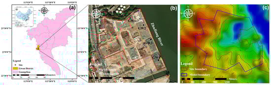
Figure 1.
Location of (a) the study site, site boundaries (red line in (b)), and model boundaries (blue line in (c)).
To investigate the soil contamination, the soil samples were taken to the laboratory for analysis. The soil samples were dried, sieved, and passed through a 2 mm mesh and were then stored for measurements. For As measurement, the soil was first digested with HCl and HNO3, and its concentrations were then measured using atomic fluorescence spectrometry (AFS, AFS-9130, Titan Instruments, China) [30]. For PAH concentration measurement, the soil was extracted using the Soxhlet extraction method, and the PAHs in the extracts were measured using gas chromatography-mass spectrometry (GC-MS, QP2010 Shimadzu, Kyoto, Japan) [31]. The measurement quality control for As was conducted using standard reference soil (GSS-5), with a determination accuracy of 97.5–100.3%. The PAHs measurement quality control was conducted using the soil spiked with standard solutions that had recovery ratios of 79–137% for benzo[a]pyrene (Bap) and 69–82% for dibenz(a,h)anthracene (Dba).
The soil at the site contained As with a concentration range of 1.6 to 210.2 mg/kg, two PAH compounds (Bap and Dba) with Bap concentrations ranging from 0.001 to 4.31 mg/kg, and a Dba concentration from 0.001 to 0.75 mg/kg. Their concentrations in groundwater were below regulatory standards: As: <10 μg/L and PAHs: <10 ng/L. Soil samples were also taken to analyze microbial communities at the site by DNA extraction, 16S rRNA sequencing, and subsequent high-throughput sequencing analysis. The detailed sampling procedure and results are provided in Supporting Materials (Text S1).
2.2. Model Framework
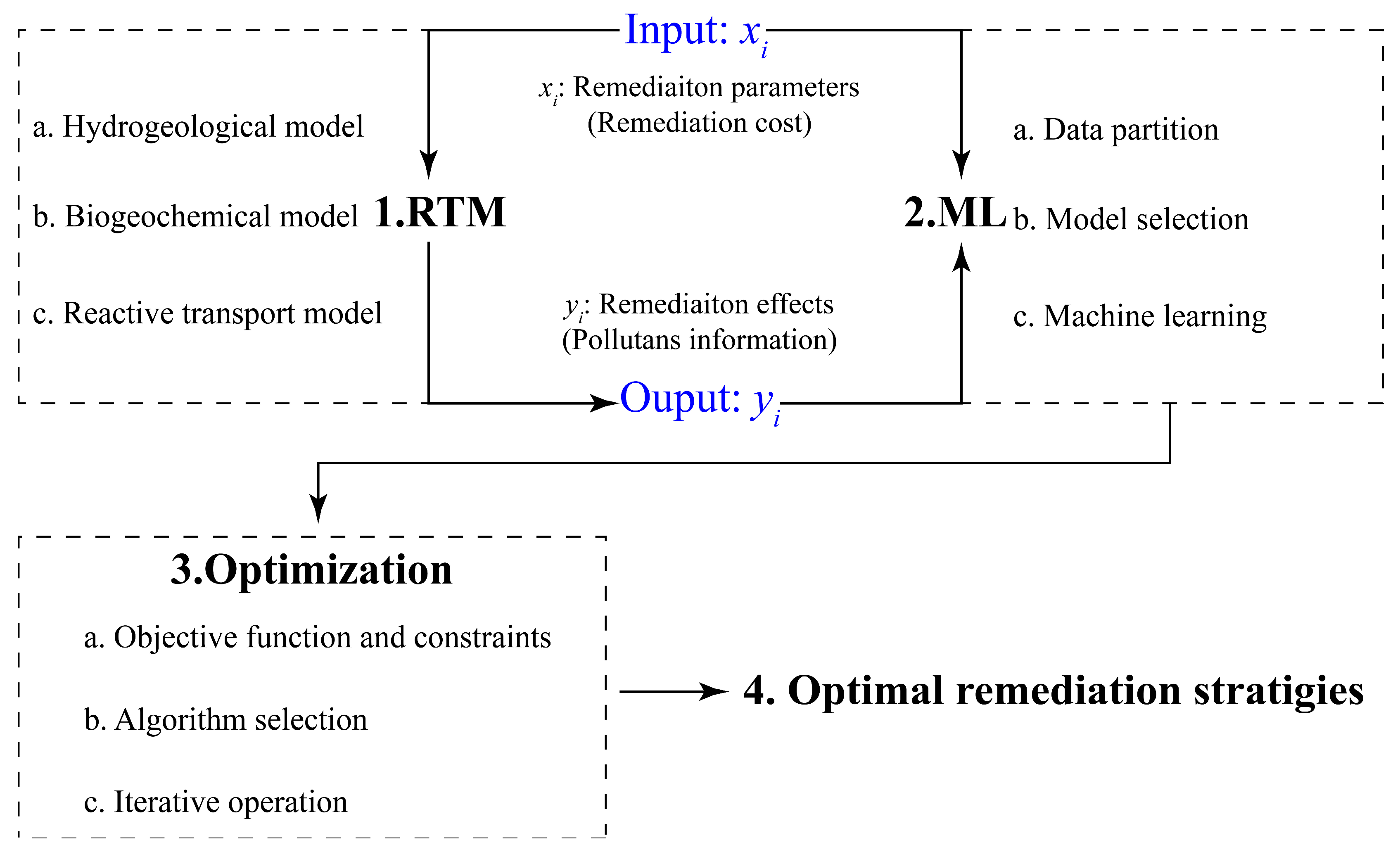
The framework for screening and optimizing remediation strategies for a contaminated site comprises three key components: RTM, ML, and optimization (Figure 2). The RTM is used to simulate the fate and transport of contaminants under various remedial conditions. The results include remediation effects (Figure 2, Yi), such as the residual soil contaminant volumes, groundwater contaminant concentrations, and contaminant discharges to nearby rivers, and remediation parameters (Figure 2, xi), such as the locations and volumes for the implementation of different remediation technologies, the types or concentrations of remediation reagents, etc., that are related to the cost of a remediation strategy. The results are used to train an ML model with a goal to establish the relationships between remediation parameters and remediation effects. The relationships are then used by an optimization algorithm to identify optimal remediation strategies under various constraints of site-specific remediation requirements. The framework is general and can be applied to any contaminated site.
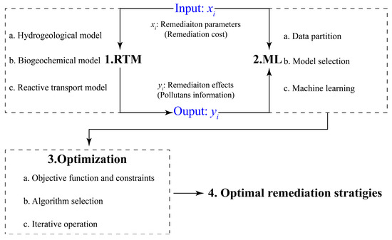
Figure 2.
A model framework for screening and optimizing remediation strategies.
2.2.1. Reactive Transport Model
A reactive transport simulation software, PFLOTRAN (v5.0, USA) [32], was used as an RTM in this study. In the software, the groundwater flow is simulated using the Richards’ equation as follows:
where φ is the porosity [-], s is the saturation degree [m3/m3], ρ is the water density [kmol/m3], q is the Darcy velocity [m/s], and Qω represents a source/sink of water [kmol/m3∙s]. The Darcy flux, q, is calculated following Darcy’s Law, where k is the intrinsic permeability [m2], kr is the relative permeability [-], μ is the viscosity [Pa∙s], P is the pressure [Pa], Wω is the molecular weight of water [kg/kmol], g is the gravity [m/s2], and z is the vertical component of the position vector [m].
The reactive transport of dissolved contaminants such as organic carbon (DOC), As, Bap, and Dba can be described as follows:
where Cj is the total concentration of component j [mol/L], Ωj is the total flux of component j [mol/(L s)], vjm is the stoichiometric coefficient of chemical component j in the mth reaction, and Rm is the mth reaction rate [mol/(L s)].
Various geochemical and biogeochemical reactions controlling the transformation of contaminants can be incorporated into the RTM. In this study, reactions related to As, Bap, and Dba were considered (Figure S2 and Table S3). Because the degradation pathways for the PAHs and As sorption and desorption are often related to iron biogeochemistry [33,34], iron redox reactions were also considered in this study. At the site, the iron(III) content in the soil, as determined by XRF, ranged from 1.6% to 5.5%.
A Monod-type model was used to describe the bioreduction of ferrihydrite, which was often treated as a surrogate for the sorbents of metal and organic contaminants in subsurface systems [35,36,37,38]:
where k2 is the oxidation rate constant [L/(mol·h)], CFe2+ is the ferrous concentration [mol/L], is the DO concentration [mol/L].
The aerobic microbial respiration was also considered in this study with the following rate expression [39,40]:
where k2 is the oxidation rate constant [L/(mol·h)], CFe2+ is the ferrous concentration [mol/L], and is the DO concentration [mol/L].
The aerobic microbial respiration was also considered in this study with the following rate expression [39,40]:
where k3 is the respiration rate constant [1/s], X is the biomass concentration [mol/L], is the DO concentration [mol/L], CDOC is the DOC concentration [mol/L], and KDOC and are, respectively, the half-saturation constants with respect to DOC and DO [mol/L].
The rate of DOC production from the transformation of particulate organic carbon (POC) is described below [39,40]:
where CPOC is the POC concentration [mol/m3], Kd,DOC is the distribution coefficient between DOC and POC [L/g], and αDOC is the mass transfer coefficient [1/h].
For PAHs, both aerobic and anaerobic biodegradation processes were considered in this study [25,41]. The aerobic reactions and rates are described as follows:
where k5 is the aerobic biodegradation rate constant [1/s], CPAHs is the PAH concentration [mol/L], KPAH,5 is the half-saturation constant with respect to PAHs [mol/L], respectively, and other variables are as described before.
The anaerobic reactions and rates are described as follows:
where k6 is the anaerobic biodegradation rates [1/s], KPAH,6 and KFe3+ are the half-saturation constants with respect to PAHs and ferrihydrite [mol/m3], respectively, is the inhibition constant during anaerobic biodegradation [mol/L], and other variables are described as before.
The co-metabolism of multi-substrate PAH biodegradation was also considered in this study using the following expression [42]:
where Ksi and Ksj are the half rate constants for the degradation of PAH compounds i and j [mol/L], and Ci and Cj are the concentrations of PAH compound i and j [mol/L], respectively.
Both As and PAHs can sorb to subsurface materials [43,44]. Their competitive sorption was derived by assuming that their sorption follows the Langmuir sorption isotherm as follows:
where KAs and KPAHs are the sorption affinity constants for As and PAHs [L/mol], respectively, CAs and CPAHs are the As and PAH concentrations in the aqueous phase [mol/L], and St is the total sorption site density [mol/m3]. The values of these parameters can be found in Table S2.
For the RTM implementation, a remediation site has to be discretized. For the target site, the high-precision data from a digital elevation map (DEM) and site characterization were used in the discretization. An unstructured triangular grid was generated by COMSOL Multiphysics software (v6.0, USA) with a denser grid in the contaminated areas. Vertically, the bedrock lies approximately 15 m below the ground surface, while contaminants are mainly located at depths of 0–3 m. Consequently, variable vertical discretization intervals were used in this study with an interval of 0.5 m, from 0 to 3 m depth, 1 m, from 3 to 5 m depth, and 5 m, from 5 to 20 m depth, resulting in a total number of the numerical grids of 86,076. The model domain covered the entire study area with the following boundary conditions: tidal water level in the nearby Zhujiang River for the eastern boundary (Figure S3b); ground surface with local precipitation infiltration at the top boundary (Figure S3a); no-flux condition at the bottom boundary where is an impermeable layer; and no-flux condition at other boundaries because they were placed at the watershed edge [45]. The measured chemical compositions in the nearby Zhujiang River water samples were used as the chemical concentration conditions at the eastern boundary. The initial concentration distributions of soil contaminants (such as As, Bap, and Dba) were derived from the site characterization and were interpolated by MATLAB R2019b. The initial As and PAH concentrations in groundwater were estimated by assuming their equilibrium with the concentrations in the soil.
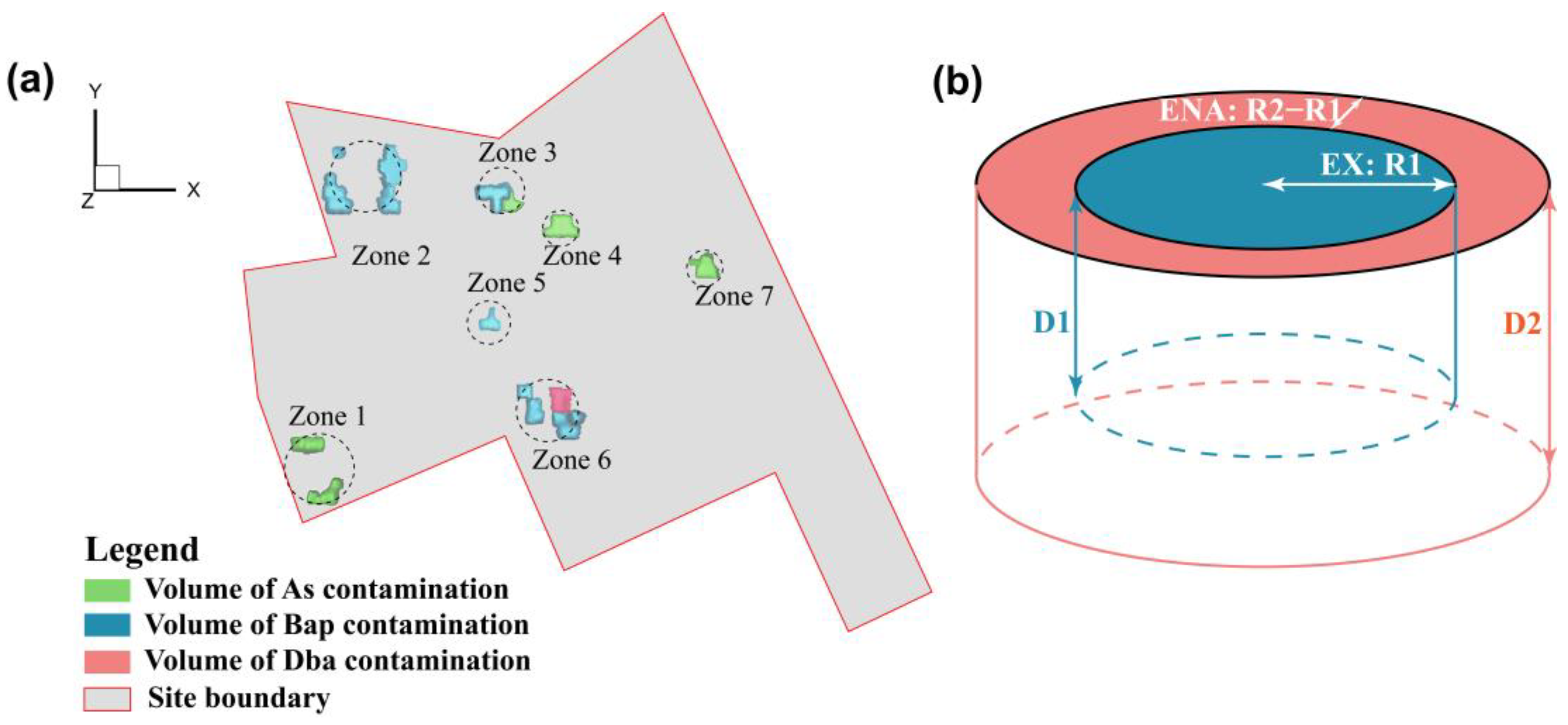
There were 7 contaminated zones to be remediated at the site (Figure 3a). For each remediation zone, the effects of individual remediation technologies were simulated using the RTM. The candidate technologies that are acceptable to local agencies include MNA, enhanced natural attenuation (ENA), in-situ stabilization, and EX. The simulation results (Figures S5–S8) indicated that only the EX treatment could meet the site remediation requirements, i.e., the groundwater concentrations of all the contaminants must be lower than drinking water standards (As <10 μg/L, PAHs <10 ng/L [46,47,48]) and the concentrations of residual soil contaminants must be below the standards of industrial land development (As <60 mg/kg, PAHs <0.55 mg/kg [49,50]). However, the volume for the EX treatment can be optimized by treating heavily contaminated soils using the EX treatment, the slightly contaminated soils with enhanced natural attenuation (ENA), and the residual contaminated soils treated with MNA. Consequently, for the subsequent simulations, the EX treatment was placed in the center of radius R1, which was the place with the highest concentrations of contaminants. The ENA was from radius R1 to R2, and the MNA for the remaining contaminated area, where the concentrations of contaminants were relatively low in each zone (Figure 3b). For each zone, R1 and R2 and the corresponding depth D1 and D2 from the ground surface were the variables to be optimized with a goal to reduce the total remediation cost. In this study, the main cost was associated with the volume for the EX and treatment under the constraints that soil and groundwater quality values meet the regulatory standards after remediation. The values for R1, R2, D1, and D2 were assumed to be independent and could be different for different remediation zones (Zone 1–7). This leads to 4 variables for each zone, yielding 28 variables to be optimized for the site with 7 remediation zones.
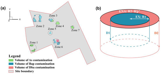
Figure 3.
Illustration of (a) 7 remediation zones and (b) remediation variables for each remediation zone where the center region with a radius R1 and depth D1 is to be treated with EX, the region from R1 to R2 with a depth of D2 to be treated with ENA, and the remaining contaminated soil outside R2 to be treated with MNA in each zone.
2.2.2. ML Model
In this study, the RTM was first used to simulate remediation effects with different combinations of the remediation technologies for the 7 remediation zones. The simulated results were used to train an ML model to establish the relationship between the inputs (variables R1, R2, D1, and D2 for 7 zones) and outputs (maximum concentrations of the contaminants in groundwater and the residual contaminated soil volumes for MNA). The reliability of the ML-based relationship was evaluated during the training process using variables R2 and RMSE. The data required for training a reliable ML-based relationship was continuously generated by the RTM until the ML model achieved a reliable accuracy. For the current case, 291 cases were simulated for training the ML model, satisfying the ratio requirement of sample size to feature size (280 cases at least) [51]. Four different ML models were evaluated in this study: ridge regression, support vector machine (SVR), random forest, and extreme gradient boosting (XGBoost). The five-fold cross-validation was used in this study to obtain a set of optimal hyperparameters for constructing the ML model, where the training and test datasets were divided at a 3:1 ratio. The model with the highest precision was chosen.
2.2.3. Optimization of Remediation Strategies
With the establishment of the ML-based relationship between the remediation input and output variables, an optimization algorithm developed at the University of Arizona (SCE-UA [52]) was used to search for optimal strategies and associated parameters by minimizing the total remediation cost (e.g., EX treatment volume) under different regulatory constraints and site requirements. The SCE-UA algorithm was chosen due to its excellent performance and efficiency in global search [53,54,55] with the detailed optimization procedure described elsewhere [56].
3. Results and Discussion
3.1. Simulated Groundwater Flow and Reactive Transport of Contaminants under Natural Conditions
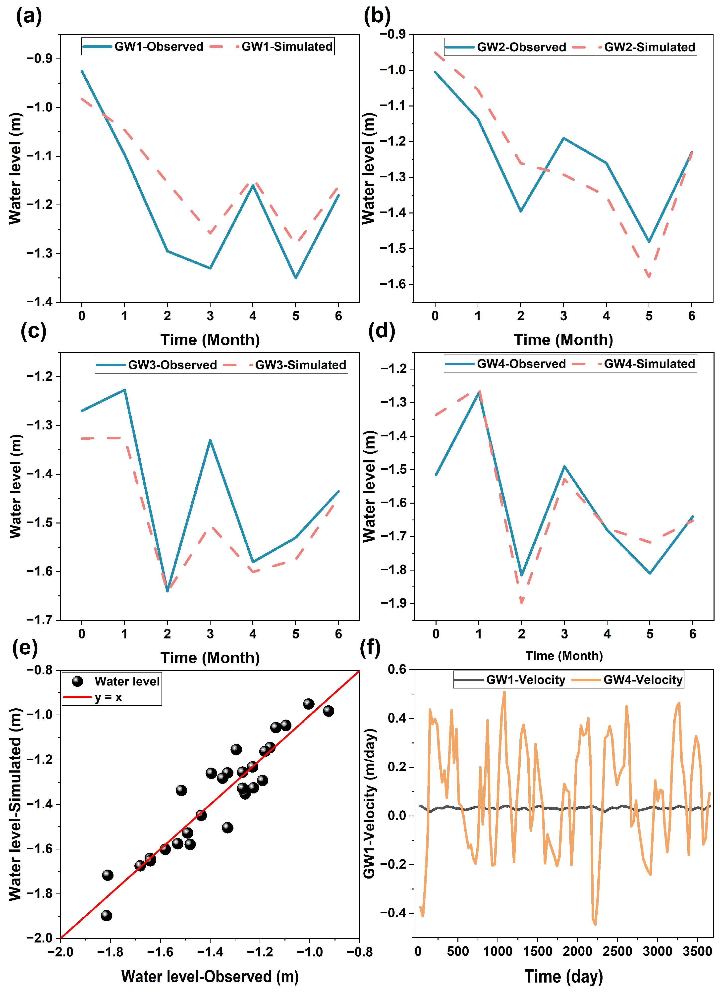
Groundwater flow fluctuated daily and seasonally, as revealed by the fluctuation of groundwater levels at the monitoring wells at the site (Figure 4 and Figure 5). The fluctuation of the groundwater levels was mainly attributed to the fluctuation of nearby river water levels as a result of tidal and seasonal precipitation events (Figure S3). The groundwater levels simulated by the RTM matched well with the observed monitoring wells with a Nash coefficient of 0.83 (Figure 4a), indicating a good agreement between the simulated and observed data [57]. The groundwater flow directions at the site changed frequently near the riverside (e.g., GW4). This change diminished with an increasing distance from the river (e.g., GW1). The frequent reversals of groundwater flow directions would increase the exchange of river water with groundwater, promoting the biogeochemical transformation of soil contaminants [58,59,60].
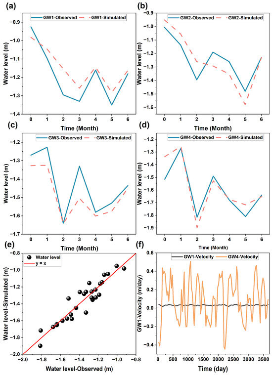
Figure 4.
Observed and simulated groundwater levels at (a–d) individual monitoring wells, (e) all observed and simulated data, and the simulated groundwater velocity at monitoring wells (f) GW1 and GW4.
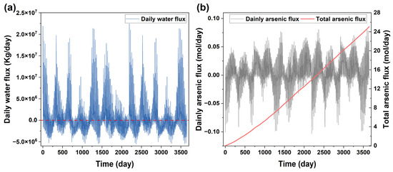
Figure 5.
The flux of water (plot (a)) and As (plot (b)) from the site to the river.
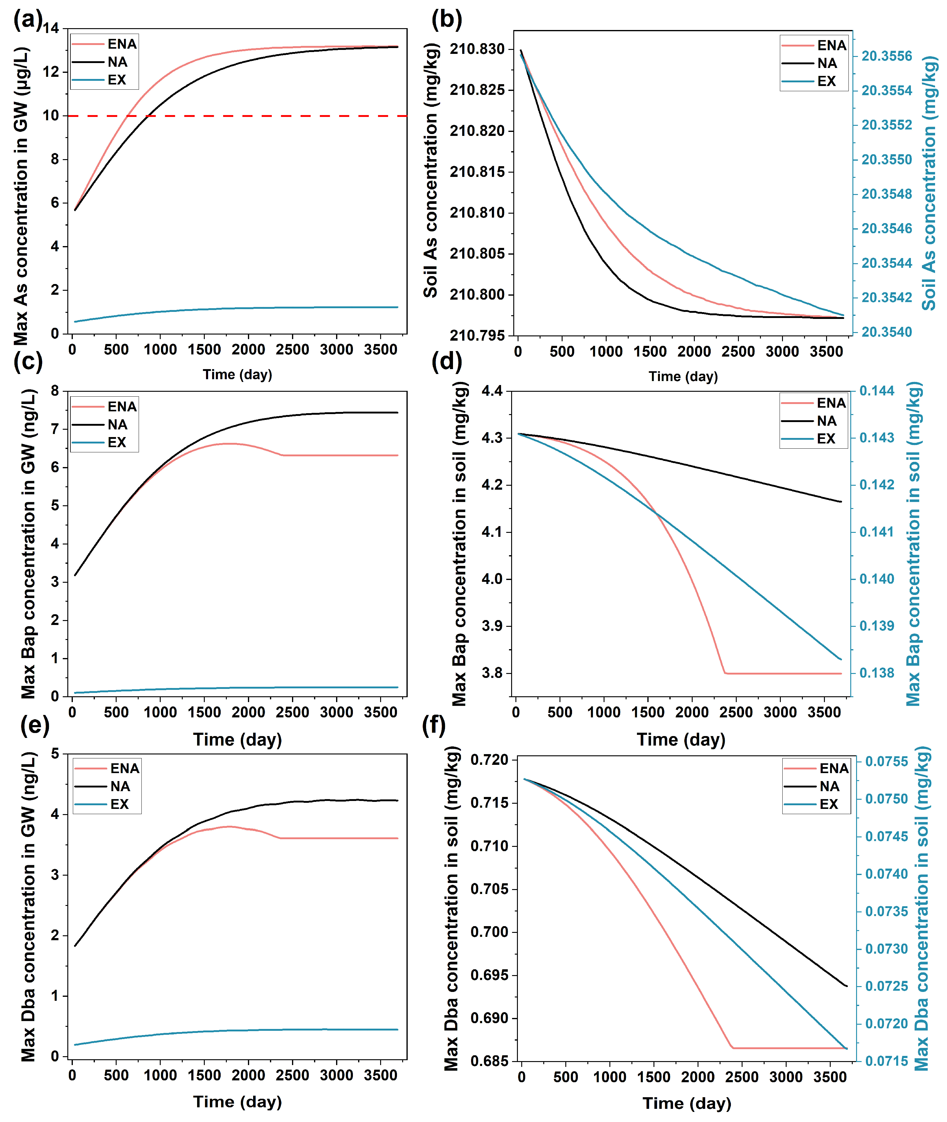
The effect of MNA was simulated to predict the fate and reactive transport of the contaminants under natural conditions. The results showed that the As concentration in groundwater gradually increased with time near the contaminant sources, reaching 13.2 μg/L after 10 years (Figure 6a and Figure S5) as a result of the slow reduction of sorbent ferrihydrite. Meanwhile, the As concentration in the soil slowly decreased as it was released to groundwater. The simulated result also showed that PAH oxidation enhanced the As release under anaerobic conditions, a phenomenon consistent with the literature reports [61,62]. The biogeochemical processes related to iron reduction and PAH biodegradation considered in this study were feasible at the site where the main microbial compositions were Proteobacteria (42–65%) and Firmicutes (23–34%) at the phylum level and Bacillus, Hydrogenophaga, and Acinetobacter at the genus level (Table 1 and Figure S2). These microorganisms can reduce iron oxides and degrade PAHs.
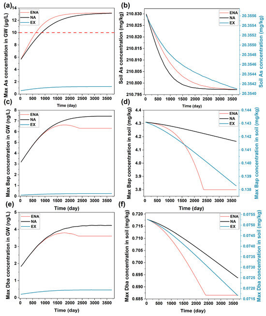
Figure 6.
The concentration changes in groundwater ((a): As, (c): Bap, (e): Dba) and soil ((b): As, (d): Bap, (f): Dba) under conditions of MNA, ENA, and EX.

Table 1.
Microorganisms and their functions at the target site.
The As flux from the site to the nearby Zhujiang River was small (Figure 5b) and did not significantly increase the As concentration in the river as it was diluted by the high water flux in the river (Figure 5a). The result indicated that the MNA could remediate the contaminant in the soils at the site without affecting the nearby river water quality. However, it could not meet the time constraint for the site that was targeted for subsequent redevelopment after remediation within a short time duration. It may also cause a problem of groundwater contamination during the long duration of the MNA. Consequently, the MNA alone was not enough to remediate the site.
The simulated concentrations of both Bap and Dba in groundwater were lower than the regulatory level (10 ng/L, Figure 6a), while their concentrations in the soil were significantly over the regulatory level (Figure 6b) during the simulation period. In the simulation, the microbial degradation of PAHs was considered. However, their solubility was low, leading to the low biodegradability of PAHs in the soil [68,69]. The results of As and PAHs both indicated that active remediation of the contaminated soil was needed for the targeted site.
3.2. Simulated Effects of Active Remediation Technologies
The effects of two active remediation technologies, ENA and EX, were individually simulated to evaluate the changes in contaminant concentrations in groundwater and soil. ENA was implemented with the addition of organic material (lactate in this study) as the electron donor and carbon source for microorganism growth [70,71]. The implementation of the ENA resulted in a faster As release rate from the soil than MNA due to the enhanced ferrihydrite reduction by microorganisms with the addition of organic matter (Figure 6a,b). The faster As release led to the earlier arrival of As concentrations in groundwater to above regulatory level, indicating that the ENA would also potentially cause groundwater contamination. The microbial degradation of Bap and Dba was also enhanced by the addition of organic matter. However, the rate decreased significantly when the added organic matter was diminished with time, indicating that it needs to be replenished continuously to maintain the degradation [72].
The EX is a simple and time-effective remediation strategy for contaminant removal [18,73,74]. The concentrations of As, Bap, and Dba after EX can both meet groundwater and soil remediation goals (Figure 6 and Figure S8). However, the cost for the EX was much higher than the MNA and ENA as it requires the excavation of a large amount of the contaminated soil and subsequent treatment. Considering the efficiency and cost of the MNA, ENA, and EX, it would be ideal to combine them with the goal of minimizing the remediation cost under the constraints of regulatory and local requirements. The remediation requirements at the site were various, including the discharge of contaminants from the site to the nearby river that would not affect river water quality, no groundwater contamination was allowed during and after the remediation, contaminant concentrations in the soil must meet regulatory criteria, and the remediation duration must meet site-redevelopment schedule. Given these requirements, a remediation strategy, as described in Figure 3, was proposed, which separated each remediation zone into three spatial regions defined by parameters R1, R2, D1, and D2. In order to determine the values of these parameters that would give the minimal remediation cost under the constraints of the remediation requirements, RTM was first used to simulate the reactive transport of contaminants with different combinations of these parameters. The data generated from the RTM simulations were then used to establish the relationships linking these parameter values with corresponding remediation costs, which were then used to find an optimal remediation strategy, as described in the next section.
3.3. Remediation Strategies and Optimization
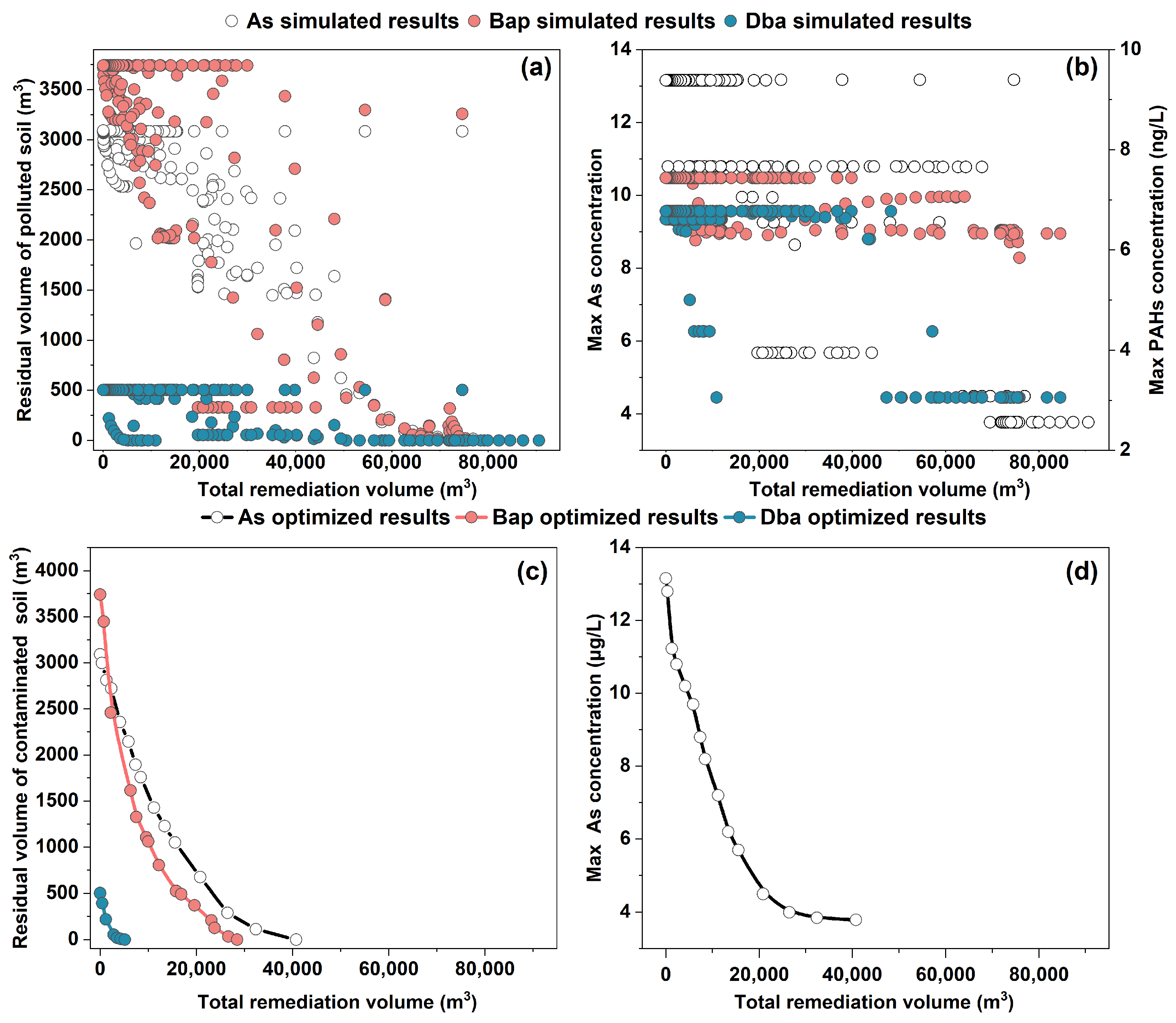
The RTM-simulated results showed that different remediation strategies, as generated by adjusting remediation parameters (R1, R2, D1, and D2) for each remediation zone, would lead to different residual volumes of the contaminated soil for subsequent MNA (Figure 7a) and different groundwater concentrations (Figure 7b) as a function of the total volume of the contaminated soil treated with EX and ENA. A larger excavated volume generally, as expected, led to lower groundwater concentrations and residual volumes of the contaminated soil. The result also showed that for a specific EX volume of the contaminated soil, groundwater concentrations and residual volumes of the contaminated soil varied. This is because the different placements of the EX zones within the contaminated areas would lead to different remediation results. The placement of the EX at a highly contaminated location within each zone led to lower groundwater concentrations and residual volumes of the contaminated soil despite the same amount of the excavated contaminated soil. These results indicated that extensive RTM simulations are required to find an optimal combination of the remediation parameters (R1, R2, D1, and D2), which would yield the lowest cost of remediation.
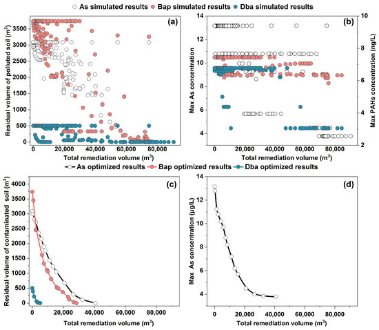
Figure 7.
Relationship between the residual volume of the contaminated soil vs. the total remediation volume of the contaminated soil (excavated volume) (a) and maximum concentrations of the contaminants in groundwater as a function of total remediation volume of the contaminated soil (b). The optimized residual volume of the contaminated soil as a function of total remediation volume from the ML-SCE-UA results (c) and the maximum As concentration in groundwater as a function of remediation volume (d).
In this study, instead of performing extensive RTM simulations, the results from a select set of simulations, as shown in Figure 7, were used to train an ML model to establish a relationship linking the remediation parameters (R1, R2, D1, and D2) with the simulated results of groundwater concentrations and residual volumes of the contaminants at the site. When properly trained, such an ML-based relationship could replace the RTM to generate simulation results from other combinations of remediation parameters (R1, R2, D1, and D2). In this study, various ML methods were compared to evaluate their performances in fitting the RTM-simulated results, as shown in Figures S9 and S10, and it was found that the XGBoost method had the best performance.
The ML-based relationship from the XGBoost method was then used by an optimization algorithm (SCE-UA) to search for an optimal combination of remediation parameters (R1, R2, D1, and D2) that would give the lowest cost of the remediation and meet the site remediation requirements (Figure 7c,d). During the optimization process, the remediation parameters (R1, R2, D1, and D2) were optimized for each contaminant (As, Bap, and Dba). The optimization results indicated that to meet the groundwater quality standard for As (<10 μg/L) at the site, 5768 m3 of the contaminated soil with the high concentration has to be excavated, while the other soil can be left for the MNA. Since the simulated groundwater concentrations of Bap and Dba are always less than the groundwater quality standards, the EX treatment of 5768 m3 of the contaminated soil with the MNA for the residual contaminated soil can meet all groundwater standards for both As and PAH contaminants. The residual contaminated soil would not pose a health risk if kept at the site despite the fact that the concentrations of the contaminants in the residual contaminated soil still exceeded the soil quality standards. If the site needs to meet both the groundwater standards and the soil standards, then the excavated volume would be 40,755 m3 for the As-contaminated soil, 21,922 m3 for the Bap-contaminated soil, and 5149 m3 for the Dba-contaminated soil. Because of the partial overlap of the soils contaminated with these contaminants (Figure 3), the total excavation volume would be less than their addition. The optimization results also showed that adding ENA with a volume of 6910 m3 would reduce the excavation volume (Table S3). The other residual contaminated soils with their contaminant concentrations above the background levels were left for MNA. The result from the optimization process indicated that the combination of EX and MNA was the most optimum method to treat the contaminated soil. EX is a time-efficient but costly technology for soil remediation, while MNA is a low-cost technology but requires a long duration of remediation action. For targeting a site for re-development, a long duration of remediation is not acceptable. The combination of the EX and MNA can have advantages and minimize the shortcomings of each technology. Here, the EX was optimized to treat the contaminated soils with high concentrations of contaminants, while the areas containing low concentrations of contaminants were left for MNA. Because the areas with low concentrations of contaminants have no risk of health risk exposure, they can be left at the site for MNA without a need for active remediation. Consequently, the combined EX and MNA can reduce the amount of the contaminated soil for EX treatment, and meanwhile, it can significantly reduce the time duration of active remediation.
Under the actual field conditions, the selection of remediation strategies should be considered under different constraints suitable to the specific sites, such as economic, environmental, and social impacts, besides the selection of remediation technologies to meet both regulatory groundwater and soil standards [75]. In this context, our framework can readily consider the different constraints during the optimization step that can be tailored to a specific site. At this site, a remediation strategy that combines EX and MNA was eventually selected to meet both groundwater and soil standards because of the current regulatory requirements for the site redevelopment. From the view of remediation cost, treating 5768 m3 of contaminated soil with EX, followed by MNA for the residual contaminated soil, was cost-effective and could reduce the cost by 91.5%, assuming that the cost for MNA is negligible compared to EX. As a validation of the approach, the simulated results of aqueous As concentrations were compared with the measured concentrations at the monitoring wells (Figure S11). The simulated results generally matched well with the measured results, indicating that the approach was effective and could be used for screening and optimizing soil remediation strategies.
A similar framework to the one reported previously [17] was used in this study, which consists of RTM, ML, and optimization algorithms. However, the previous study focused more on the development of the framework itself with a demonstration site having a relatively simple contamination history and biogeochemistry. The current study focused on solving a real and complex problem using the framework on a site contaminated with both organic and inorganic contaminants, featuring multiple contamination zones as shown in Table 2. This significantly increases the complexity of the biogeochemistry and optimization, providing a realistic demonstration of the framework’s application and an optimal remediation strategy for the site. Additionally, the simulated results presented here were compared with the measured data monitored in this study, validating the effectiveness of the framework.
Table 2.
The comparison between the current and previous study.
4. Prospect and Limitation
The framework used in this study was general and can be adapted to other contaminated sites by incorporating site-specific data such as hydrology, geochemistry, and biogeochemistry, as well as the site requirements and constraints for remediation. Being module-based, the framework allows any advancements in each module to be readily updated. For example, the ML part is rapidly advancing, becoming more intelligent in handling high-dimensional and large-scale datasets [76,77,78]. Such an advance can be readily incorporated into the ML module in the framework. Similarly, the optimization method is also fast evolving with progress, such as swarm intelligence algorithms, hybrid algorithms, and nature-inspired algorithms that are computationally efficient and fast converging with a strong global search capability [79,80,81]. Such advances can also be incorporated into the framework by updating the optimization module. One major limitation of the application of the framework is that extensive site characterization of hydrology and biogeochemistry properties is required to obtain a reliable set of input data for the RTM, which is the foundation of the framework. The high-precision prediction of remediation effects from different potential remediation approaches relies on the accuracy of simulated RTM results, which will ultimately determine the selection of an optimal remediation strategy during the optimization step.
5. Conclusions
This study developed a numerical approach that can be used for screening and optimizing remediation strategies to clean up contaminants in soil and groundwater systems. The approach consisted of three components: (1) RTM simulations of the fate and transport of contaminants under natural and remedial conditions for preliminary screening of potential remediation technologies; (2) using the RTM simulation data to train an ML model for establishing the relationships linking remediation parameters, such as sizes and locations, for the implementation of specific remediation technologies with remediation effects, such as residual concentrations in groundwater and soil, their subsequent changes after remediation, and the costs associated with the implementation of remediation technologies, such as the excavation volume of the contaminated soil; and (3) using the relationship and global optimization algorithm to find optimal remediation strategies. Using a field site that was contaminated with As and PAHs as an example, this study demonstrated the application of the approach in finding optimal remediation strategies. The optimal approach selected from this study under the constraint of local regulations and site requirements was successfully implemented.
While a site co-contaminated with As and PAHs was demonstrated, the developed approach is general for screening and optimizing remediation strategies at any other sites. One important adaptation in applying the approach to other sites is the biogeochemical part in the RTM, including biogeochemical reactions and parameters, which may be specific to the target site. The ML part of the approach is to reduce computational cost because extensive RTM simulations are required to generate enough data for establishing the relationships between remediation parameters and remediation effects. Such relationships can be established with a limited number of RTM simulations when ML is used. The ML part can be ignored if the remediation site is relatively small and biogeochemical reactions are relatively simple to describe the fate and transport of contaminants. For a large remediation site or a site contaminated with multiple contaminants with complex geochemical behaviors, the ML part is recommended to be included.
Supplementary Materials
The following supporting information can be downloaded at: https://www.mdpi.com/article/10.3390/pr12061157/s1, Text S1: Methods for DNA extraction and microbial structure analysis; Figure S1: Geological stratigraphy of the borehole at the site; Figure S2: Relative abundance of microbial organisms on phylum level (a), genus level (b) and net analysis among microbial communities at genus level (c); Figure S3: Seasonal precipitation (a) and river stage fluctuations (b) of Zhujiang River; Figure S4: The locations of the cross-sections for As (black dotted line) and PAHs (Bap and Dba for blue dotted line) in demonstrating the simulation results shown in Figures S3–S6; Figure S5: The concentration changes of As (a,c,g), Bap (b,e,h), and Dba (c,f,i) in groundwater during 10-year simulation under MNA conditions; Figure S6: The concentration changes of As (a,c,g), Bap (b,e,h), and Dba (c,f,i) in groundwater during 10-year simulation under ENA conditions; Figure S7: The concentration changes of As (a,c,g), Bap (b,e,h), and Dba (c,f,i) in groundwater during 10-year simulation under in-situ stabilization conditions; Figure S8: The concentration changes of As (a,c,g), Bap (b,e,h), and Dba (c,f,i) in groundwater during 10-year simulation under EX conditions; Figure S9: The performance of various ML models in fitting the RTM data, which was evaluated by index of R2 (a) and root mean square error (RMSE) (b); Figure S10: The relationship between the groundwater concentration and residual volume of the contaminated soil ((a), As; (b), Bap; (c), Dba) obtained from RTM and ML (XGBoost); Figure S11: The measured and simulated concentrations (As, Bap, and Dba) at three monitoring wells: (a) GW1, (b) GW2, (c) GW4, and (d) in all wells combined; Table S1: Parameters for the biogeochemical reactions used in this study; Table S2: Hydrogeological parameters used in this study; Table S3: The optimal remediation parameters under different remediation requirements. Refs. [40,41,82,83,84,85,86,87,88,89] are cited in Supplementary Materials.
Author Contributions
Conceptualization, Methodology, Software, Formal analysis, Investigation, Writing—original draft, Visualization, B.Z.; Methodology, Software, Validation, Investigation, X.W.; Conceptualization, Writing—review & editing, Supervision, Funding acquisition, C.L. All authors have read and agreed to the published version of the manuscript.
Funding
This work was funded by the National Key Research and Development Program of China (project No.: 2019YFC1803903), Program for Guangdong Introducing Innovative and Entrepreneurial Teams (2017ZT07Z479) and by High level of special funds (G03050K001).
Data Availability Statement
All data and materials supporting the findings of this study are available upon reasonable request.
Acknowledgments
This work was also supported by the Center for Computational Science and Engineering at Southern University of Science and Technology.
Conflicts of Interest
The authors declare no conflicts of interest.
References
- Li, T.K.; Liu, Y.; Lin, S.J.; Liu, Y.Z.; Xie, Y.F. Soil Pollution Management in China: A Brief Introduction. Sustainability 2019, 11, 556. [Google Scholar] [CrossRef]
- Orecchio, S. Assessment of polycyclic aromatic hydrocarbons (PAHs) in soil of a Natural Reserve (Isola delle Femmine) (Italy) located in front of a plant for the production of cement. J. Hazard. Mater. 2010, 173, 358–368. [Google Scholar] [CrossRef] [PubMed]
- Wang, D.G.; Alaee, M.; Byer, J.; Liu, Y.J.; Tian, C.G. Fugacity approach to evaluate the sediment-water diffusion of polycyclic aromatic hydrocarbons. J. Environ. Monit. 2011, 13, 1589–1596. [Google Scholar] [CrossRef] [PubMed]
- Zhang, H.B.; Luo, Y.M.; Wong, M.H.; Zhao, Q.G.; Zhang, G.L. Distributions and concentrations of PAHs in Hong Kong soils. Environ. Pollut. 2006, 141, 107–114. [Google Scholar] [CrossRef] [PubMed]
- Zhao, F.J.; Ma, Y.B.; Zhu, Y.G.; Tang, Z.; McGrath, S.P. Soil Contamination in China: Current Status and Mitigation Strategies. Environ. Sci. Technol. 2015, 49, 750–759. [Google Scholar] [CrossRef] [PubMed]
- Han, L.J.; Li, J.S.; Xue, Q.; Che, Z.; Zhou, Y.Y.; Poon, C.S. Bacterial-induced mineralization (BIM) for soil solidification and heavy metal stabilization: A critical review. Sci. Total Environ. 2020, 746, 140967. [Google Scholar] [CrossRef] [PubMed]
- Hussain, A.; Rehman, F.; Rafeeq, H.; Waqas, M.; Asghar, A.; Afsheen, N.; Rahdar, A.; Bilal, M.; Iqbal, H.M.N. In-situ, Ex-situ, and nano-remediation strategies to treat polluted soil, water, and air-A review. Chemosphere 2022, 289, 133252. [Google Scholar] [CrossRef]
- Shah, V.; Daverey, A. Phytoremediation: A multidisciplinary approach to clean up heavy metal contaminated soil. Environ. Technol. Innov. 2020, 18, 100774. [Google Scholar] [CrossRef]
- Senila, M.; Cadar, O.; Senila, L.; Angyus, B.S. Simulated Bioavailability of Heavy Metals (Cd, Cr, Cu, Pb, Zn) in Contaminated Soil Amended with Natural Zeolite Using Diffusive Gradients in Thin-Films (DGT) Technique. Agriculture 2022, 12, 321. [Google Scholar] [CrossRef]
- Sarkar, D.; Ferguson, M.; Datta, R.; Birnbaum, S. Bioremediation of petroleum hydrocarbons in contaminated soils: Comparison of biosolids addition, carbon supplementation, and monitored natural attenuation. Environ. Pollut. 2005, 136, 187–195. [Google Scholar] [CrossRef]
- Falciglia, P.P.; Giustra, M.G.; Vagliasindi, F.G.A. Low-temperature thermal desorption of diesel polluted soil: Influence of temperature and soil texture on contaminant removal kinetics. J. Hazard. Mater. 2011, 185, 392–400. [Google Scholar] [CrossRef] [PubMed]
- Zhang, B.; Guo, Y.; Huo, J.; Xie, H.; Xu, C.; Liang, S. Combining chemical oxidation and bioremediation for petroleum polluted soil remediation by BC-nZVI activated persulfate. Chem. Eng. J. 2020, 382, 123055. [Google Scholar] [CrossRef]
- Schwartz, M.O.; Kgomanyane, J. Modelling natural attenuation of heavy-metal groundwater contamination in the Selebi-Phikwe mining area, Botswana. Environ. Geol. 2008, 54, 819–830. [Google Scholar] [CrossRef]
- Zhao, H.R.; Xia, B.C.; Qin, J.Q.; Zhang, J.Y. Hydrogeochemical and mineralogical characteristics related to heavy metal attenuation in a stream polluted by acid mine drainage: A case study in Dabaoshan Mine, China. J. Environ. Sci. 2012, 24, 979–989. [Google Scholar] [CrossRef] [PubMed]
- Chen, C.; Zhang, X.M.; Chen, J.A.; Chen, F.Y.; Li, J.H.; Chen, Y.C.; Hou, H.B.; Shi, F. Assessment of site contaminated soil remediation based on an input output life cycle assessment. J. Clean. Prod. 2020, 263, 121422. [Google Scholar] [CrossRef]
- Gong, Y.Y.; Zhao, D.Y.; Wang, Q.L. An overview of field-scale studies on remediation of soil contaminated with heavy metals and metalloids: Technical progress over the last decade. Water Res. 2018, 147, 440–460. [Google Scholar] [CrossRef] [PubMed]
- Wang, X.; Li, R.; Tian, Y.; Zhang, B.W.; Zhao, Y.; Zhang, T.T.; Liu, C.X. A Computational Framework for Design and Optimization of Risk-Based Soil and Groundwater Remediation Strategies. Processes 2022, 10, 2572. [Google Scholar] [CrossRef]
- Liu, L.W.; Li, W.; Song, W.P.; Guo, M.X. Remediation techniques for heavy metal-contaminated soils: Principles and applicability. Sci. Total Environ. 2018, 633, 206–219. [Google Scholar] [CrossRef]
- Pavel, L.V.; Gavrilescu, M. Overview of Ex Situ Decontamination Techniques for Soil Cleanup. Environ. Eng. Manag. J. 2008, 7, 815–834. [Google Scholar] [CrossRef]
- Rajendran, S.; Priya, T.A.K.; Khoo, K.S.; Hoang, T.K.A.; Ng, H.S.; Munawaroh, H.S.H.; Karaman, C.; Orooji, Y.; Show, P.L. A critical review on various remediation approaches for heavy metal contaminants removal from contaminated soils. Chemosphere 2022, 287, 132369. [Google Scholar] [CrossRef]
- Rahman, S.; Rahman, I.M.M.; Hasegawa, H. Management of arsenic-contaminated excavated soils: A review. J. Environ. Manag. 2023, 346, 118943. [Google Scholar] [CrossRef] [PubMed]
- Locatelli, L.; Binning, P.J.; Sanchez-Vila, X.; Sondergaard, G.L.; Rosenberg, L.; Bjerg, P.L. A simple contaminant fate and transport modelling tool for management and risk assessment of groundwater pollution from contaminated sites. J. Contam. Hydrol. 2019, 221, 35–49. [Google Scholar] [CrossRef]
- Masi, M.; Ceccarini, A.; Iannelli, R. Multispecies reactive transport modelling of electrokinetic remediation of harbour sediments. J. Hazard. Mater. 2017, 326, 187–196. [Google Scholar] [CrossRef]
- Qin, X.S.; Huang, G.H.; He, L. Simulation and optimization technologies for petroleum waste management and remediation process control. J. Environ. Manag. 2009, 90, 54–76. [Google Scholar] [CrossRef]
- Lu, G.P.; Clement, T.P.; Zheng, C.M.; Wiedemeier, T.H. Natural attenuation of BTEX compounds: Model development and field-scale application. Groundwater 1999, 37, 707–717. [Google Scholar] [CrossRef] [PubMed]
- Olson, M.R.; Sale, T.C. Implications of soil mixing for NAPL source zone remediation: Column studies and modeling of field-scale systems. J. Contam. Hydrol. 2015, 177, 206–219. [Google Scholar] [CrossRef] [PubMed]
- Hansen, S.K.; Pandey, S.; Karra, S.; Vesselinov, V.V. CHROTRAN 1.0: A mathematical and computational model for in situ heavy metal remediation in heterogeneous aquifers. Geosci. Model. Dev. 2017, 10, 4525–4538. [Google Scholar] [CrossRef]
- Verardo, E.; Atteia, O.; Rouvreau, L.; Siade, A.; Prommer, H. Identifying remedial solutions through optimal bioremediation design under real-world field conditions. J. Contam. Hydrol. 2021, 237, 103751. [Google Scholar] [CrossRef]
- Yadav, B.; Ch, S.; Mathur, S.; Adamowski, J. Estimation of in-situ bioremediation system cost using a hybrid Extreme Learning Machine (ELM)-particle swarm optimization approach. J. Hydrol. 2016, 543, 373–385. [Google Scholar] [CrossRef]
- Tao, C.; Wang, Y.; Cui, W.; Zou, B.; Zou, Z.; Tu, Y. A transferable spectroscopic diagnosis model for predicting arsenic contamination in soil. Sci. Total Environ. 2019, 669, 964–972. [Google Scholar] [CrossRef]
- Pongpiachan, S.; Hattayanone, M.; Tipmanee, D.; Suttinun, O.; Khumsup, C.; Kittikoon, I.; Hirunyatrakul, P. Chemical characterization of polycyclic aromatic hydrocarbons (PAHs) in 2013 Rayong oil spill-affected coastal areas of Thailand. Environ. Pollut. 2018, 233, 992–1002. [Google Scholar] [CrossRef]
- Hammond, G.E.; Lichtner, P.C.; Mills, R.T. Evaluating the performance of parallel subsurface simulators: An illustrative example with PFLOTRAN. Water Resour. Res. 2014, 50, 208–228. [Google Scholar] [CrossRef] [PubMed]
- Herbel, M.; Fendorf, S. Biogeochemical processes controlling the speciation and transport of arsenic within iron coated sands. Chem. Geol. 2006, 228, 16–32. [Google Scholar] [CrossRef]
- Zhao, Z.W.; Meng, Y.; Yuan, Q.K.; Wang, Y.H.; Lin, L.M.; Liu, W.B.; Luan, F.B. Microbial mobilization of arsenic from iron-bearing clay mineral through iron, arsenate, and simultaneous iron-arsenate reduction pathways. Sci. Total Environ. 2021, 763, 144613. [Google Scholar] [CrossRef] [PubMed]
- Campos-Pereira, H.; Kleja, D.B.; Sjöstedt, C.; Ahrens, L.; Klysubun, W.; Gustafsson, J.P. The Adsorption of Per- and Polyfluoroalkyl Substances (PFASs) onto Ferrihydrite Is Governed by Surface Charge. Environ. Sci. Technol. 2020, 54, 15722–15730. [Google Scholar] [CrossRef]
- Meng, S.; Wang, H.L.; Liu, H.; Yang, C.H.; Wei, Y.; Hou, D.L. Evaluation of the ability of ferrihydrite to bind heavy metal ions: Based on formation environment, adsorption reversibility and ageing. Appl. Geochem. 2014, 45, 114–119. [Google Scholar] [CrossRef]
- Qian, G.R.; Chen, W.; Lim, T.T.; Chui, P. In-situ stabilization of Pb, Zn, Cu, Cd and Ni in the multi-contaminated sediments with ferrihydrite and apatite composite additives. J. Hazard. Mater. 2009, 170, 1093–1100. [Google Scholar] [CrossRef]
- Zhang, P.; Liu, A.J.; Huang, P.; Min, L.J.; Sun, H.W. Sorption and molecular fractionation of biochar-derived dissolved organic matter on ferrihydrite. J. Hazard. Mater. 2020, 392, 122260. [Google Scholar] [CrossRef] [PubMed]
- Gu, C.H.; Hornberger, G.M.; Mills, A.L.; Herman, J.S.; Flewelling, S.A. Nitrate reduction in streambed sediments: Effects of flow and biogeochemical kinetics. Water Resour. Res. 2007, 43. [Google Scholar] [CrossRef]
- Liu, Y.Y.; Xu, F.; Liu, C.X. Coupled Hydro-Biogeochemical Processes Controlling Cr Reductive Immobilization in Columbia River Hyporheic Zone. Environ. Sci. Technol. 2017, 51, 1508–1517. [Google Scholar] [CrossRef]
- Geng, X.L.; Boufadel, M.C.; Lee, K.; Abrams, S.; Suidan, M. Biodegradation of subsurface oil in a tidally influenced sand beach: Impact of hydraulics and interaction with pore water chemistry. Water Resour. Res. 2015, 51, 3193–3218. [Google Scholar] [CrossRef]
- Guha, S.; Peters, C.A.; Jaffe, P.R. Multisubstrate biodegradation kinetics of naphthalene, phenanthrene, and pyrene mixtures. Biotechnol. Bioeng. 1999, 65, 491–499. [Google Scholar] [CrossRef]
- Raven, K.P.; Jain, A.; Loeppert, R.H. Arsenite and arsenate adsorption on ferrihydrite: Kinetics, equilibrium, and adsorption envelopes. Environ. Sci. Technol. 1998, 32, 344–349. [Google Scholar] [CrossRef]
- Tunega, D.; Zaoui, A. Adsorption of polycyclic aromatic hydrocarbons on FeOOH polymorphs: A theoretical study. Surf. Sci. 2021, 706, 121795. [Google Scholar] [CrossRef]
- Reggiani, P.; Rientjes, T.H.M. Flux parameterization in the representative elementary watershed approach: Application to a natural basin. Water Resour. Res. 2005, 41. [Google Scholar] [CrossRef]
- Chakraborti, D.; Rahman, M.M.; Das, B.; Murrill, M.; Dey, S.; Mukherjee, S.C.; Dhar, R.K.; Biswas, B.K.; Chowdhury, U.K.; Roy, S.; et al. Status of groundwater arsenic contamination in Bangladesh: A 14-year study report. Water Res. 2010, 44, 5789–5802. [Google Scholar] [CrossRef]
- Podgorski, J.; Berg, M. Global threat of arsenic in groundwater. Science 2020, 368, 845–850. [Google Scholar] [CrossRef] [PubMed]
- Zhang, Y.; Zhang, L.F.; Huang, Z.P.; Li, Y.N.; Li, J.F.; Wu, N.; He, J.H.; Zhang, Z.Z.; Liu, Y.Q.; Niu, Z.G. Pollution of polycyclic aromatic hydrocarbons (PAHs) in drinking water of China: Composition, distribution and influencing factors. Ecotoxicol. Environ. Safe 2019, 177, 108–116. [Google Scholar] [CrossRef]
- Xie, K.T.; Xie, N.E.; Liao, Z.Y.; Luo, X.S.; Peng, W.J.; Yuan, Y. Bioaccessibility of arsenic, lead, and cadmium in contaminated mining/smelting soils: Assessment, modeling, and application for soil environment criteria derivation. J. Hazard. Mater. 2023, 443, 130321. [Google Scholar] [CrossRef]
- Zhao, Y.Y.; Duan, F.A.; Cui, Z.J.; Hong, J.L.; Ni, S.Q. Insights into the vertical distribution of the microbiota in steel plant soils with potentially toxic elements and PAHs contamination after 60 years operation: Abundance, structure, co-occurrence network and functionality. Sci. Total Environ. 2021, 786, 147338. [Google Scholar] [CrossRef]
- Zhu, J.-J.; Yang, M.; Ren, Z.J. Machine Learning in Environmental Research: Common Pitfalls and Best Practices. Environ. Sci. Technol. 2023, 57, 17671–17689. [Google Scholar] [CrossRef] [PubMed]
- Duan, Q.Y.; Sorooshian, S.; Gupta, V.K. Optimal Use of the Sce-Ua Global Optimization Method for Calibrating Watershed Models. J. Hydrol. 1994, 158, 265–284. [Google Scholar] [CrossRef]
- Gopala, S.P.; Kawamura, A.; Amaguchi, H.; Takasaki, T.; Azhikodan, G. A bootstrap approach for the parameter uncertainty of an urban-specific rainfall-runoff model. J. Hydrol. 2019, 579, 124195. [Google Scholar] [CrossRef]
- Green, C.H.; van Griensven, A. Autocalibration in hydrologic modeling: Using SWAT2005 in small-scale watersheds. Environ. Model. Softw. 2008, 23, 422–434. [Google Scholar] [CrossRef]
- Qi, W.; Zhang, C.; Fu, G.T.; Zhou, H.C. Quantifying dynamic sensitivity of optimization algorithm parameters to improve hydrological model calibration. J. Hydrol. 2016, 533, 213–223. [Google Scholar] [CrossRef]
- Duan, Q.Y.; Ajami, N.K.; Gao, X.G.; Sorooshian, S. Multi-model ensemble hydrologic prediction using Bayesian model averaging. Adv. Water Resour. 2007, 30, 1371–1386. [Google Scholar] [CrossRef]
- Moriasi, D.N.; Gitau, M.W.; Pai, N.; Daggupati, P. Hydrologic and Water Quality Models: Performance Measures and Evaluation Criteria. Trans. ASABE 2015, 58, 1763–1785. [Google Scholar] [CrossRef]
- Harvey, J.W.; Bohlke, J.K.; Voytek, M.A.; Scott, D.; Tobias, C.R. Hyporheic zone denitrification: Controls on effective reaction depth and contribution to whole-stream mass balance. Water Resour. Res. 2013, 49, 6298–6316. [Google Scholar] [CrossRef]
- Shuai, P.; Chen, X.Y.; Song, X.H.; Hammond, G.E.; Zachara, J.; Royer, P.; Ren, H.Y.; Perkins, W.A.; Richmond, M.C.; Huang, M.Y. Dam Operations and Subsurface Hydrogeology Control Dynamics of Hydrologic Exchange Flows in a Regulated River Reach. Water Resour. Res. 2019, 55, 2593–2612. [Google Scholar] [CrossRef]
- Son, K.; Fang, Y.L.; Gomez-Velez, J.D.; Byun, K.; Chen, X.Y. Combined Effects of Stream Hydrology and Land Use on Basin-Scale Hyporheic Zone Denitrification in the Columbia River Basin. Water Resour. Res. 2022, 58, e2021WR031131. [Google Scholar] [CrossRef]
- Meckenstock, R.U.; Boll, M.; Mouttaki, H.; Koelschbach, J.S.; Tarouco, P.C.; Weyrauch, P.; Dong, X.Y.; Himmelberg, A.M. Anaerobic Degradation of Benzene and Polycyclic Aromatic Hydrocarbons. J. Microbiol. Biotechnol. 2016, 26, 92–118. [Google Scholar] [CrossRef] [PubMed]
- Shen, X.F.; Dong, W.H.; Wan, Y.Y.; Feng, K.J.; Liu, Y.; Wei, Y.J. Influencing mechanisms of siderite and magnetite, on naphthalene biodegradation: Insights from degradability and mineral surface structure. J. Environ. Manag. 2021, 299, 113648. [Google Scholar] [CrossRef] [PubMed]
- Chen, C.; Zhang, Z.; Xu, P.; Hu, H.; Tang, H. Anaerobic biodegradation of polycyclic aromatic hydrocarbons. Environ. Res. 2023, 223, 115472. [Google Scholar] [CrossRef]
- Wang, N.; Xue, X.M.; Juhasz, A.L.; Chang, Z.Z.; Li, H.B. Biochar increases arsenic release from an anaerobic paddy soil due to enhanced microbial reduction of iron and arsenic. Environ. Pollut. 2017, 220, 514–522. [Google Scholar] [CrossRef] [PubMed]
- Zada, S.; Zhou, H.; Xie, J.; Hu, Z.; Ali, S.; Sajjad, W.; Wang, H. Bacterial degradation of pyrene: Biochemical reactions and mechanisms. Int. Biodeterior. Biodegrad. 2021, 162, 105233. [Google Scholar] [CrossRef]
- Yan, Z.; Zhang, Y.; Wu, H.; Yang, M.; Zhang, H.; Hao, Z.; Jiang, H. Isolation and characterization of a bacterial strain: Hydrogenophaga sp. PYR1 for anaerobic pyrene and benzo[a]pyrene biodegradation. RSC Adv. 2017, 7, 46690–46698. [Google Scholar] [CrossRef]
- Brzeszcz, J.; Kaszycki, P. Aerobic bacteria degrading both n-alkanes and aromatic hydrocarbons: An undervalued strategy for metabolic diversity and flexibility. Biodegradation 2018, 29, 359–407. [Google Scholar] [CrossRef] [PubMed]
- Baltrons, O.; Lopez-Mesas, M.; Vilaseca, M.; Gutierrez-Bouzan, C.; Le Derf, F.; Portet-Koltalo, F.; Palet, C. Influence of a mixture of metals on PAHs biodegradation processes in soils. Sci. Total Environ. 2018, 628–629, 150–158. [Google Scholar] [CrossRef]
- Eggen, T.; Majcherczyk, A. Removal of polycyclic aromatic hydrocarbons (PAH) in contaminated soil by white rot fungus Pleurotus ostreatus. Int. Biodeterior. Biodegrad. 1998, 41, 111–117. [Google Scholar] [CrossRef]
- Blazquez-Palli, N.; Rosell, M.; Varias, J.; Bosch, M.; Soler, A.; Vicent, T.; Marco-Urrea, E. Multi-method assessment of the intrinsic biodegradation potential of an aquifer contaminated with chlorinated ethenes at an industrial area in Barcelona (Spain). Environ. Pollut. 2019, 244, 165–173. [Google Scholar] [CrossRef]
- Schneidewind, U.; Haest, P.J.; Atashgahi, S.; Maphosa, F.; Hamonts, K.; Maesen, M.; Calderer, M.; Seuntjens, P.; Smidt, H.; Springael, D.; et al. Kinetics of dechlorination by Dehalococcoides mccartyi using different carbon sources. J. Contam. Hydrol. 2014, 157, 25–36. [Google Scholar] [CrossRef]
- Geng, X.L.; Pan, Z.; Boufadel, M.C.; Ozgokmen, T.; Lee, K.; Zhao, L. Simulation of oil bioremediation in a tidally influenced beach: Spatiotemporal evolution of nutrient and dissolved oxygen. J. Geophys. Res.-Oceans 2016, 121, 2385–2404. [Google Scholar] [CrossRef]
- Khan, S.; Naushad, M.; Lima, E.C.; Zhang, S.X.; Shaheen, S.M.; Rinklebe, J. Global soil pollution by toxic elements: Current status and future perspectives on the risk assessment and remediation strategies-A review. J. Hazard. Mater. 2021, 417, 126039. [Google Scholar] [CrossRef]
- Tomei, M.C.; Daugulis, A.J. Ex Situ Bioremediation of Contaminated Soils: An Overview of Conventional and Innovative Technologies. Crit. Rev. Environ. Sci. Technol. 2013, 43, 2107–2139. [Google Scholar] [CrossRef]
- Naseri-Rad, M.; Berndtsson, R.; Persson, K.M.; Nakagawa, K. INSIDE: An efficient guide for sustainable remediation practice in addressing contaminated soil and groundwater. Sci. Total Environ. 2020, 740, 139879. [Google Scholar] [CrossRef]
- Pyo, J.; Hong, S.M.; Kwon, Y.S.; Kim, M.S.; Cho, K.H. Estimation of heavy metals using deep neural network with visible and infrared spectroscopy of soil. Sci. Total Environ. 2020, 741, 140162. [Google Scholar] [CrossRef] [PubMed]
- Janga, J.K.; Reddy, K.R.; Raviteja, K.V.N.S. Integrating artificial intelligence, machine learning, and deep learning approaches into remediation of contaminated sites: A review. Chemosphere 2023, 345, 140476. [Google Scholar] [CrossRef] [PubMed]
- Yan, H.; Zheng, Q.; Zeng, L. Conditional generative adversarial networks for groundwater contamination characterization and source identification. J. Hydrol. 2024, 632, 130900. [Google Scholar] [CrossRef]
- Zhang, Y.; Chen, H.; Lv, M.; Hou, Z.; Wang, Y. Swarm intelligence machine-learning-assisted progressive global optimization of DNAPL-contaminated aquifer remediation strategy. Water Supply 2023, 23, 1250–1266. [Google Scholar] [CrossRef]
- Pham, Q.B.; Tran, D.A.; Ha, N.T.; Islam, A.R.M.T.; Salam, R. Random forest and nature-inspired algorithms for mapping groundwater nitrate concentration in a coastal multi-layer aquifer system. J. Clean. Prod. 2022, 343, 130900. [Google Scholar] [CrossRef]
- Yaseen, Z.M.; Melini Wan Mohtar, W.H.; Homod, R.Z.; Alawi, O.A.; Abba, S.I.; Oudah, A.Y.; Togun, H.; Goliatt, L.; Ul Hassan Kazmi, S.S.; Tao, H. Heavy metals prediction in coastal marine sediments using hybridized machine learning models with metaheuristic optimization algorithm. Chemosphere 2024, 352, 141329. [Google Scholar] [CrossRef] [PubMed]
- Liu, H.; Hu, Z.; Zhou, M.; Zhang, H.; Li, Z.; Zhang, H.; Hu, J.; Yao, X.; Lou, L.; Xi, C.; et al. Airborne microorganisms exacerbate the formation of atmospheric ammonium and sulfate. Environ. Pollut. 2020, 263, 114293. [Google Scholar] [CrossRef] [PubMed]
- Lu, H.; Li, Y.; Shan, X.; Abbas, G.; Zeng, Z.; Kang, D.; Wang, Y.; Zheng, P.; Zhang, M. A holistic analysis of ANAMMOX process in response to salinity: From adaptation to collapse. Sep. Purif. Technol. 2019, 215, 342–350. [Google Scholar] [CrossRef]
- Yang, C.; Zhang, Y.K.; Liu, Y.Y.; Yang, X.F.; Liu, C.X. Model-Based Analysis of the Effects of Dam-Induced River Water and Groundwater Interactions on Hydro-Biogeochemical Transformation of Redox Sensitive Contaminants in a Hyporheic Zone. Water Resour. Res. 2018, 54, 5973–5985. [Google Scholar] [CrossRef]
- Huang, K.; Liu, Y.Y.; Yang, C.; Duan, Y.H.; Yang, X.F.; Liu, C.X. Identification of Hydrobiogeochemical Processes Controlling Seasonal Variations in Arsenic Concentrations Within a Riverbank Aquifer at Jianghan Plain, China. Water Resour. Res. 2018, 54, 4294–4308. [Google Scholar] [CrossRef]
- Zarnetske, J.P.; Haggerty, R.; Wondzell, S.M.; Bokil, V.A.; González-Pinzón, R. Coupled transport and reaction kinetics control the nitrate source-sink function of hyporheic zones. Water Resour. Res. 2012, 48. [Google Scholar] [CrossRef]
- Urbain, V.; Mobarry, B.; de Silva, V.; Stahl, D.A.; Rittmann, B.E.; Manem, J. Integration of performance, molecular biology and modeling to describe the activated sludge process. Water Sci. Technol. 1998, 37, 223–229. [Google Scholar] [CrossRef]
- Herold, M.; Greskowiak, J.; Ptak, T.; Prommer, H. Modelling of an enhanced PAH attenuation experiment and associated biogeochemical changes at a former gasworks site in southern Germany. J. Contam. Hydrol. 2011, 119, 99–112. [Google Scholar] [CrossRef]
- Brauner, J.S.; Widdowson, M.A. Sequential electron acceptor model for evaluation of bioremediation of petroleum hydrocarbon contaminants in groundwater. Ann. N. Y. Acad. Sci. 1997, 829, 263–279. [Google Scholar] [CrossRef]


Disclaimer/Publisher’s Note: The statements, opinions and data contained in all publications are solely those of the individual author(s) and contributor(s) and not of MDPI and/or the editor(s). MDPI and/or the editor(s) disclaim responsibility for any injury to people or property resulting from any ideas, methods, instructions or products referred to in the content. |
© 2024 by the authors. Licensee MDPI, Basel, Switzerland. This article is an open access article distributed under the terms and conditions of the Creative Commons Attribution (CC BY) license (https://creativecommons.org/licenses/by/4.0/).