
Leveraging Designed Simulations and Machine Learning to Develop a Surrogate Model for Optimizing the Gas–Downhole Water Sink–Assisted Gravity Drainage (GDWS-AGD) Process to Improve Clean Oil Production


Abstract
:1. Introduction
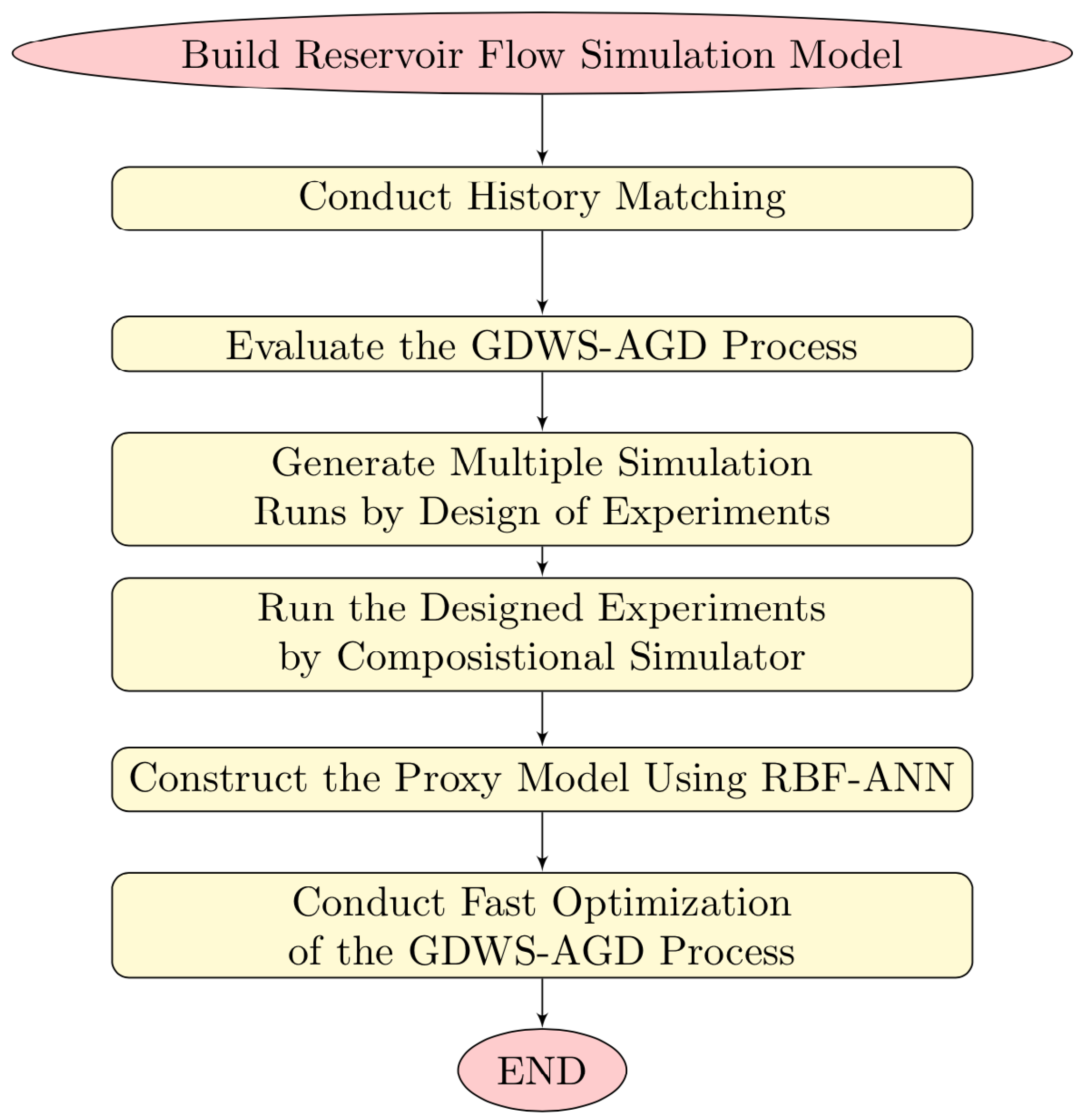
- Develop a comprehensive and detailed compositional reservoir flow simulation to evaluate the reservoir production using the immiscible GDWS-AGD process for a prediction period of 10 years.
- The Design of Experiments–Latin Hypercube Sampling (DoE-LHS) approach was used to create many computer experiments (realizations) that were included in the compositional reservoir simulation to calculate the flow response factor, which is the recovery factor. More specifically, the DoE-LHS technique was employed to generate several simulation runs by varying the values of each controlling parameter on the gas injection, oil, and water production activities.
- The controlling parameters were adjusted systematically to minimize the number of simulation runs needed to obtain the optimal scenarios for implementing CO2 injection.
- Subsequently, following the implementation of numerous simulation scenarios, the DoE-LHS method was integrated to produce a simplified surrogate approach (metamodel) as an alternative to the compositional reservoir model.
- The radial basis function neural networks (RBF-ANNs) were effectively utilized to construct a proxy model that acts as a computationally efficient alternative to the complex compositional reservoir simulation.
2. Gas and Downhole Water Sink–Assisted Gravity Drainage (GDWS-AGD) Process
3. Compositional Reservoir Simulation of the GDWS-AGD Process
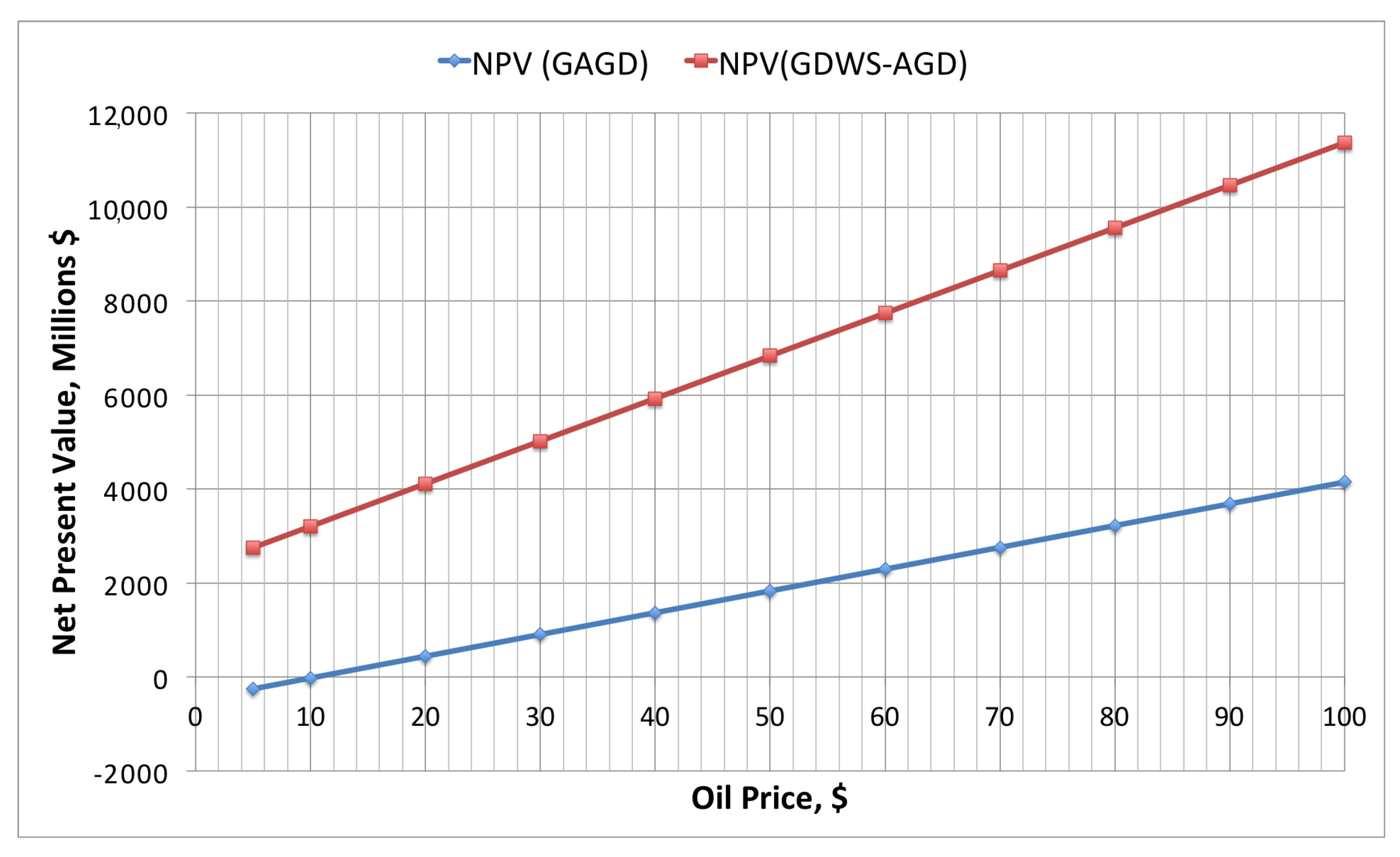
- NPV: net present value, USD.
- Oil price (): USD per STB.
- Gas price (): USD 3.0 per MSCf.
- Water handling cost (): USD 1 per STB.
- Gas injection cost (): USD 2.15 per MSCF.
- OPEX: the operational expenditures (USD 1.25–1.5/STB of oil), which include staff salaries, daily energy requirements, fuel and transportation, well workover, maintenance, and other facility improvements.
- CAPEX: the capital expenditures for drilling, completion, cementing, perforation, stimulation, and rig movement. In this paper, the CAPEX was set based on the costs of drilling vertical and horizontal wells in addition to the surface facilities for gas injection. According to the current average cost ranges in the Rumaila field, the drilling cost of one vertical well is USD 5 million, and for a horizontal well, it is USD 10 million. There was USD 35 million for the gas injection facilities.
- i: the interest rate.
4. Recovery Optimization of the GDWS-AGD Process
4.1. Optimization Approaches
4.2. GDWS-AGD Process Optimization
5. Summary and Conclusions
Author Contributions
Funding
Data Availability Statement
Acknowledgments
Conflicts of Interest
Abbreviations
| MAXSTO | aximum oil production rate in the oil wells |
| MINBHP | Minimum bottom hole pressure in the oil wells |
| MAXBHG | Maximum gas injection rate in the injection wells |
| MAXBHP | Maximum bottom hole injection pressure in the injection wells |
| MAXSTW | Maximum production rate in the water sink wells |
| MINBHPw | Minimum bottom hole pressure in the water sink wells |
| STB/DAY | Stock tank barrels of oil per day |
| SCF/DAY | Standard cubic feet of gas per day |
| MSCf | Thousands of standard cubic feet |
| NPV | Net present value |
| Oil price in USD per STB | |
| Gas price in USD per MSCf | |
| Water handling cost in USD 1 per STB | |
| Gas injection cost in USD per MSCF | |
| OPEX | The operational expenditures |
| CAPEX | The capital expenditures |
| i | The interest rate |
| Adjusted R-squared | |
| n | The number of designed experiments |
| k | The number of operational decision variables |
References
- Al-Mudhafar, W.J.; Wojtanowicz, A.K.; Rao, D.N. Hybrid Process of Gas and Downhole Water Sink-Assisted Gravity Drainage (GDWS-AGD) to Enhance Oil Recovery in Reservoirs with Water Coning. In Proceedings of the Carbon Management Technology Conference, Houston, TX, USA, 17–20 July 2017. [Google Scholar] [CrossRef]
- Qin, W.; Luo, P.; Meng, J.; Li, H.; Mao, T.; Wojtanowicz, A.K.; Feng, M. Successful Field Trials for Water Control in High Water Cut Wells Using an Improved Downhole Water Sink/Drainage System. In Proceedings of the Abu Dhabi International Petroleum Exhibition and Conference, Abu Dhabi, United Arab Emirates, 13–16 November 2017. [Google Scholar] [CrossRef]
- Kulkarni, M.M.; Rao, D.N. Experimental Investigation of Miscible and Immiscible Water-Alternating-Gas (WAG) Process Performance. J. Pet. Sci. Eng. 2005, 48, 1–20. [Google Scholar] [CrossRef]
- Al-Mudhafar, W.J.; Rao, D.N.; McCreery, E.B. Evaluation of Immiscible CO2 Enhance Oil Recovery through the CGI, WAG, and GAGD Processes in South Rumaila Oil Field. In Proceedings of the The 79th EAGE Conference and Exhibition, Paris, France, 11–16 June 2017. [Google Scholar] [CrossRef]
- Mahmoud, T.; Rao, D.N. Range of Operability of Gas-Assisted Gravity Drainage Process. Society of Petroleum Engineers. In Proceedings of the SPE Symposium on Improved Oil Recovery, Tulsa, OK, USA, 20–23 April 2008. [Google Scholar] [CrossRef]
- Al-Mudhafar, W.J.; Rao, D.N. Lessons Learned from the Field-Scale Simulation of the Gas-Assisted Gravity Drainage (GAGD) Process in Heterogeneous Sandstone Oil Reservoirs. In Proceedings of the SPE Western Regional Meeting, Bakersfield, CA, USA, 23–27 April 2017. [Google Scholar]
- Wojtanowicz, A.K. Down-Hole Water Sink Technology for Water Coning Control in Wells; Louisiana State University: Baton Rouge, LA, USA, 2006; Wiertnictwo Nafta Gaz, TOM 23/1; pp. 575–586. Available online: http://journals.bg.agh.edu.pl/WIERTNICTWO/2006-01/W_2006_1_63.pdf (accessed on 12 February 2024).
- Wojtanowicz, A.K.; Xu, H.; Bassiouni, Z.A. Oilwell Coning Control using Dual Completion with Tailpipe Water Sink. In Proceedings of the SPE Production Operation Symposium, Oklahoma, OK, USA, 7–9 April 1991. [Google Scholar] [CrossRef]
- Al-Mudhafar, W.J. Statistical Reservoir Characterization, Simulation, and Optimization Of Field Scale-Gas Assisted Gravity Drainage (GAGD) Process with Uncertainty Assessments. Ph.D. Dissertation, Louisiana State University, Baton Rouge, LA, USA, 2016. [Google Scholar]
- Ampomah, W.; Balch, R.S.; Cather, M.; Will, R.; Gunda, D.; Dai, Z.; Soltanian, M.R. Optimum design of CO2 storage and oil recovery under geological uncertainty. Appl. Energy 2017, 195, 80–92. [Google Scholar] [CrossRef]
- Vanegas Prada, J.W.; Cunha, L.B. Prediction of SAGD Performance Using Response Surface Correlations Developed by Experimental Design Techniques. J. Can. Pet. Technol. 2008, 47, 58. [Google Scholar] [CrossRef]
- Jaber, A.K.; Awang, M.B.; Stephen, K.D. Proxy modelling for rapid optimisation of miscible CO2-WAG injection in heterogeneous clastic reservoirs: A case study from Southern Iraqi oil fields. Int. J. Oil Gas Coal Technol. 2021, 26, 263–280. [Google Scholar] [CrossRef]
- Yeten, B.; Castellini, A.; Guyaguler, B.; Chen, W.H.A. Comparison Study on Experimental Design and Response Surface Methodologies. In Proceedings of the SPE Reservoir Simulation Symposium, The Woodlands, TX, USA, 31 January–2 February 2005. [Google Scholar] [CrossRef]
- Zerpa, L.E.; Queipo, N.V.; Pintos, S.; Tillero, E.; Alter, D. An Efficient Response Surface Approach for the Optimization of ASP Flooding Processes: ASP Pilot Project LL-03 Reservoir. In Proceedings of the SPE Latin American & Caribbean Petroleum Engineering Conference, Buenos Aires, Argentina, 15–18 April 2007. [Google Scholar] [CrossRef]
- Ansari, E.; Hughes, R. Response surface method for assessing energy production from geopressured geothermal reservoirs. Geotherm Energy 2016, 4, 15. [Google Scholar] [CrossRef]
- Zubarev, D.I. Pros and Cons of Applying a Proxy Model as a Substitute for Full Reservoir Simulations. In Proceedings of the SPE Annual Technical Conference and Exhibition, New Orleans, LA, USA, 4–7 October 2009. [Google Scholar] [CrossRef]
- Lee, T.H.; Lee, C.S.; Jung, J.; Kim, H.-W.; Hong, S.; Choi, J. Prediction of the Motion of Tracked Vehicle On Soft Soil Using Kriging Metamodel. In Proceedings of the Fifth ISOPE Ocean Mining Symposium, Tsukuba, Japan, 15–19 September 2003. [Google Scholar]
- Badru, O.; Kabir, C.S. Well Placement Optimization in Field Development. In Proceedings of the SPE Annual Technical Conference and Exhibition, Denver, CO, USA, 10–12 October 2003. [Google Scholar] [CrossRef]
- Zangl, G.; Graf, T.; Al-Kinani, A. Proxy Modeling in Production Optimization. In Proceedings of the SPE Europec/EAGE Annual Conference and Exhibition, Vienna, Austria, 12–15 June 2006. [Google Scholar] [CrossRef]
- Guyaguler, B.; Horne, R.N.; Rogers, L.; Rosenzweig, J.J. Optimization of Well Placement in a Gulf of Mexico Waterflooding Project. In Proceedings of the SPE Annual Technical Conference and Exhibition, Dallas, TX, USA, 1–4 October 2000. [Google Scholar] [CrossRef]
- Haghighat Sefat, M.; Salahshoor, K.; Jamialahmadi, M.; Vahdani, H. The Development of Techniques for the Optimization of Water-flooding Processes in Petroleum Reservoirs Using a Genetic Algorithm and Surrogate Modeling Approach. Energy Sources Part A Recovery Util. Environ. Eff. 2014, 36, 1175–1185. [Google Scholar] [CrossRef]
- Zhong, Z.; Sun, A.Y.; Ren, B.; Wang, Y. A Deep-Learning-Based Approach for Reservoir Production Forecast under Uncertainty. SPE J. 2021, 26, 1314–1340. [Google Scholar] [CrossRef]
- Ampomah, W.; Balch, R.S.; Grigg, R.B.; Cather, M.; Will, R.A.; Lee, S.Y. Optimization of CO2-EOR Process in Partially Depleted Oil Reservoirs. In Proceedings of the SPE Western Regional Meeting, Anchorage, AK, USA, 23–26 May 2016. [Google Scholar] [CrossRef]
- Fedutenko, E.; Yang, C.; Card, C.; Nghiem, L.X. Time-Dependent Proxy Modeling of SAGD Process. In Proceedings of the SPE Heavy Oil Conference-Canada, Calgary, AB, Canada, 11–13 June 2013. [Google Scholar] [CrossRef]
- Fedutenko, E.; Yang, C.; Card, C.; Naghiem, L. Optimization of SAGD Process Accounting for Geological Uncertainties Using Proxy Models. In Proceedings of the CSPG/CSEG/CWLS GeoConvention, Calgary, AB, Canada, 6–12 May 2013. [Google Scholar]
- Yang, C.; Card, C.; Nghiem, L.X.; Fedutenko, E. Robust optimization of SAGD operations under geological uncertainties. In Proceedings of the SPE Reservoir Simulation Symposium, The Woodlands, TX, USA, 21–23 February 2011. [Google Scholar] [CrossRef]
- Vo Thanh, H.; Dashtgoli, D.S.; Zhang, H.; Min, B. Machine-learning-based prediction of oil recovery factor for experimental CO2-Foam chemical EOR: Implications for carbon utilization projects. Energy 2023, 278, 127860. [Google Scholar] [CrossRef]
- Goodwin, N. Bridging the Gap Between Deterministic and Probabilistic Uncertainty Quantification Using Advanced Proxy Based Methods. In Proceedings of the SPE Reservoir Simulation Symposium, Houston, TX, USA, 23–25 February 2015. [Google Scholar] [CrossRef]
- He, Q.; Mohaghegh, S.D.; Liu, Z. Reservoir Simulation Using Smart Proxy in SACROC Unit-Case Study. In Proceedings of the SPE Eastern Regional Meeting, Canton, OH, USA, 13–15 September 2016. [Google Scholar] [CrossRef]
- Avansi, G.D. Use of Proxy Models in the Selection of Production Strategy and Economic Evaluation of Petroleum Fields. In Proceedings of the SPE Annual Technical Conference and Exhibition, New Orleans, LA, USA, 4–7 October 2009. [Google Scholar] [CrossRef]
- Dalton, C.A.; Broussard, M.B.; Al-Mudhafar, W.J. Proxy-Based Optimization of Hydraulic Fracturing Design in Horizontal Wells Through CO2 Flooding in Shale Oil Reservoirs. In Proceedings of the 51st U.S. Rock Mechanics/Geomechanics Symposium, San Francisco, CA, USA, 25–28 June 2017; Available online: https://www.onepetro.org/conference-paper/ARMA-2017-0737 (accessed on 12 February 2024).
- Hassani, H.; Sarkheil, H.; Foroud, T.; Karimpooli, S. A Proxy Modeling Approach to Optimization Horizontal Well Placement; American Rock Mechanics Association: Alexandria, VA, USA, 2011. [Google Scholar]
- White, C.D.; Royer, S.A. Experimental Design as a Framework for Reservoir Studies. In Proceedings of the SPE Reservoir Simulation Symposium, Houston, TX, USA, 3–5 February 2003. [Google Scholar] [CrossRef]
- Osterloh, W.T. Use of Multiple-Response Optimization to Assist Reservoir Simulation Probabilistic Forecasting and History Matching. In Proceedings of the SPE Annual Technical Conference and Exhibition, Denver, CO, USA, 21–24 September 2008. [Google Scholar] [CrossRef]
- Al-Mudhafar, W.J.; Dalton, C.A.; Al Musabeh, M.I. Metamodeling via Hybridized Particle Swarm with Polynomial and Splines Regression for Optimization of CO2-EOR in Unconventional Oil Reservoirs. In Proceedings of the SPE Reservoir Characterization and Simulation Conference and Exhibition, Abu Dhabi, United Arab Emirates, 8–10 May 2017. [Google Scholar] [CrossRef]
- Al-Mudhafar, W.J.; Rao, D.N. Proxy-Based Metamodeling Optimization of the Gas-Assisted Gravity Drainage GAGD Process in Heterogeneous Sandstone Reservoirs. In Proceedings of the SPE Western Regional Meeting, Bakersfield, CA, USA, 23–27 April 2017. [Google Scholar] [CrossRef]
- Hamdi, H.; Hajizadeh, Y.; Costa Sousa, M. Population-based sampling methods for geological well testing. Comput. Geosci. 2015, 19, 1089. [Google Scholar] [CrossRef]
- Ghaderi, S.M.; Clarkson, C.R.; Chen, S. Optimization of WAG Process for Coupled CO2 EOR-Storage in Tight Oil Formations: An Experimental Design Approach. In Proceedings of the SPE Canadian Unconventional Resources Conference, Calgary, AB, Canada, 30 October–1 November 2012. [Google Scholar] [CrossRef]
- White, C.D.; Willis, B.J.; Narayanan, K.; Dutton, S.P. Identifying and Estimating Significant Geologic Parameters with Experimental Design. SPE J. 2001, 6, 311–324. [Google Scholar] [CrossRef]
- Vo Thanh, H.; Sugai, Y.; Nguele, R.; Sasaki, K. Robust optimization of CO2 sequestration through a water alternating gas process under geological uncertainties in Cuu Long Basin. Vietnam. J. Nat. Gas Sci. Eng. 2020, 76, 103208. [Google Scholar] [CrossRef]
- Mathiassen, O.M. CO2 as Injection Gas for Enhanced Oil Recovery and Estimation of the Potential on the Norwegian Continental Shelf. Master’s Thesis, Norwegian University of Science and Technology, Stavanger, Norway, 2003. [Google Scholar]
- Rao, D.N.; Ayirala, S.C.; Kulkarni, M.M.; Sharma, A.P. Development of Gas Assisted Gravity Drainage (GAGD) Process for Improved Light Oil Recovery. In Proceedings of the SPE/DOE Symposium on Improved Oil Recovery, Tulsa, OK, USA, 21–24 April 2004. [Google Scholar] [CrossRef]
- CMG. The Computer Modeling Group’s Reservoir Simulation Manual; CMG: Calgary, AB, Canada, 2015. [Google Scholar]
- Hagoort, J. Oil Recovery by Gravity Drainage. SPE J. 1980, 20, 139–150. [Google Scholar] [CrossRef]
- Ahmed, T.; Meehan, D.N. Advanced Reservoir Management and Engineering, 2nd ed; Gulf Professional Publishing: Woburn, MA, USA, 2011. [Google Scholar] [CrossRef]
- Zanganeh, M.N.; Kam, S.I.; LaForce, T.; Rossen, W.R.R. The Method of Characteristics Applied to Oil Displacement by Foam. SPE J. 2011, 16, 8–23. [Google Scholar] [CrossRef]
- Liu, H.; Chen, Z.; Shen, L.; Guo, X.; Ji, D. Well modelling methods in thermal reservoir simulation. Oil Gas Sci. Technol.—Rev. IFP Energies Nouv. 2020, 75, 63. [Google Scholar] [CrossRef]
- Bittencourt, A.C.; Horne, R.N. Reservoir development and design optimization. In Proceedings of the SPE Annual Technical Conference and Exhibition, San Antonio, TX, USA, 5–8 October 1997. [Google Scholar] [CrossRef]
- Han, X.; Zhong, L.; Wang, X.; Liu, Y.; Wang, H. Well Placement and Control Optimization of Horizontal Steamflooding Wells Using Derivative-Free Algorithms. SPE Res. Eval. Eng. 2021, 24, 174–193. [Google Scholar] [CrossRef]
- Al-Mudhafar, W.J.; Rao, D.N.; Srinivasan, S. Reservoir sensitivity analysis for heterogeneity and anisotropy effects quantification through the cyclic CO2-Assisted Gravity Drainage EOR process—A case study from South Rumaila oil field. Fuel 2018, 221, 455–468. [Google Scholar] [CrossRef]
- Amudo, C.; Graf, T.; Dandekar, R.R.; Randle, J.M. The Pains and Gains of Experimental Design and Response Surface Applications in Reservoir Simulation Studies. In Proceedings of the SPE Reservoir Simulation Symposium, Houston, TX, USA, 2–4 February 2009. [Google Scholar] [CrossRef]
- Lazic, Z.R. Design of Experiments in Chemical Engineering; Wiley-Vch: Hoboken, NJ, USA, 2006. [Google Scholar]
- Dutta, S.; Gandomi, A.H. Chapter 15—Design of Experiments for Uncertainty Quantification Based on Polynomial Chaos Expansion Metamodels. In Handbook of Probabilistic Models; Samui, P., Bui, D.T., Chakraborty, S., Deo, R.C., Eds.; Butterworth-Heinemann: Woburn, MA, USA, 2020; pp. 369–381. [Google Scholar] [CrossRef]
- Stein, M. Large Sample Properties of Simulations Using Latin Hypercube Sampling. Technometrics 1987, 29, 143–151. [Google Scholar] [CrossRef]
- Bhat, C.R. Quasi-Random Maximum Simulated Likelihood Estimation of the Mixed Multinomial Logit Model. Transp. Res. Part B: Methodol. 2001, 35, 677–693. [Google Scholar] [CrossRef]
- McKay, M.D.; Beckman, R.J.; Conover, W.J. A Comparison of Three Methods for Selecting Values of Input Variables in the Analysis of Output from a Computer Code. Technometrics 1979, 21, 239–245. [Google Scholar] [CrossRef]
- Stocki, R. A method to improve design reliability using optimal Latin hypercube sampling. Comput. Assist. Mech. Eng. Sci. 2005, 12, 87–105. [Google Scholar]
- Orr, M.J.L. Introduction to Radial Basis Function Networks. 1996. Available online: http://www.anc.ed.ac.uk/~mjo/papers/intro.ps (accessed on 12 February 2024).
- Tatar, A.; Naseri, S.; Sirach, N.; Lee, M.; Bahadori, A. Prediction of reservoir brine properties using radial basis function (RBF) neural network. Petroleum 2015, 1, 349–357. [Google Scholar] [CrossRef]
- You, J.; Ampomah, W.; Sun, Q.; Kutsienyo, E.J.; Balch, R.S.; Dai, Z.; Cather, M.; Zhang, X. Machine learning based co-optimization of carbon dioxide sequestration and oil recovery in CO2-EOR project. J. Clean. Prod. 2020, 260, 120866. [Google Scholar] [CrossRef]
- Zhang, X.Y.; Trame, M.N.; Lesko, L.J.; Schmidt, S. Sobol Sensitivity Analysis: A Tool to Guide the Development and Evaluation of Systems Pharmacology Models. CPT Pharmacomet. Syst. Pharmacol. 2015, 4, 69–79. [Google Scholar] [CrossRef]
- Al-Obaidi, D.A.; Al-Mudhafar, W.J.; Al-Jawad, M.S. Experimental evaluation of Carbon Dioxide-Assisted Gravity Drainage process (CO2-AGD) to improve oil recovery in reservoirs with strong water drive. Fuel 2022, 324 Pt A, 124409. [Google Scholar] [CrossRef]
- Al-Obaidi, D.A.; Al-Mudhafar, W.J.; Hussein, H.H.; Rao, D.N. Experimental influence assessments of water drive and gas breakthrough through the CO2-assisted gravity drainage process in reservoirs with strong aquifers. Fuel 2024, 370, 131873. [Google Scholar] [CrossRef]


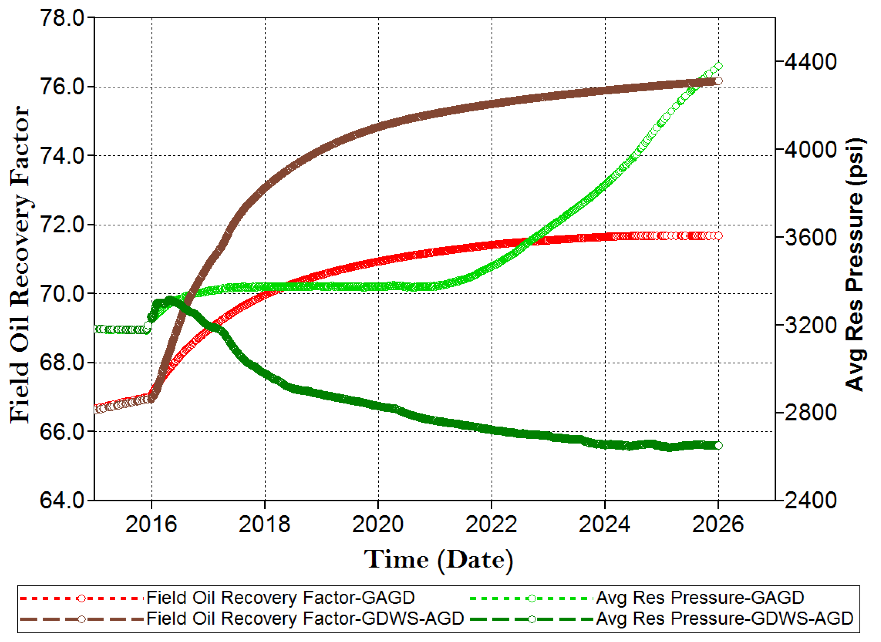
| Response | GAGD | GDWS-AGD (Base Case) |
| Oil Recovery | 71.6744% | 76.3675% |
| Parameters | ||
| MAXSTO, STB/DAY | 500,000 | 500,000 |
| MINBHP, PSI | 2000 | 2660 |
| MAXBHG, SCF/DAY | 5,000,000 | 5,000,000 |
| MAXBHP, PSI | 3200 | 4000 |
| MAXSTW, STB/DAY | 400,000 | |
| MINBHPw, PSI | 1000 |
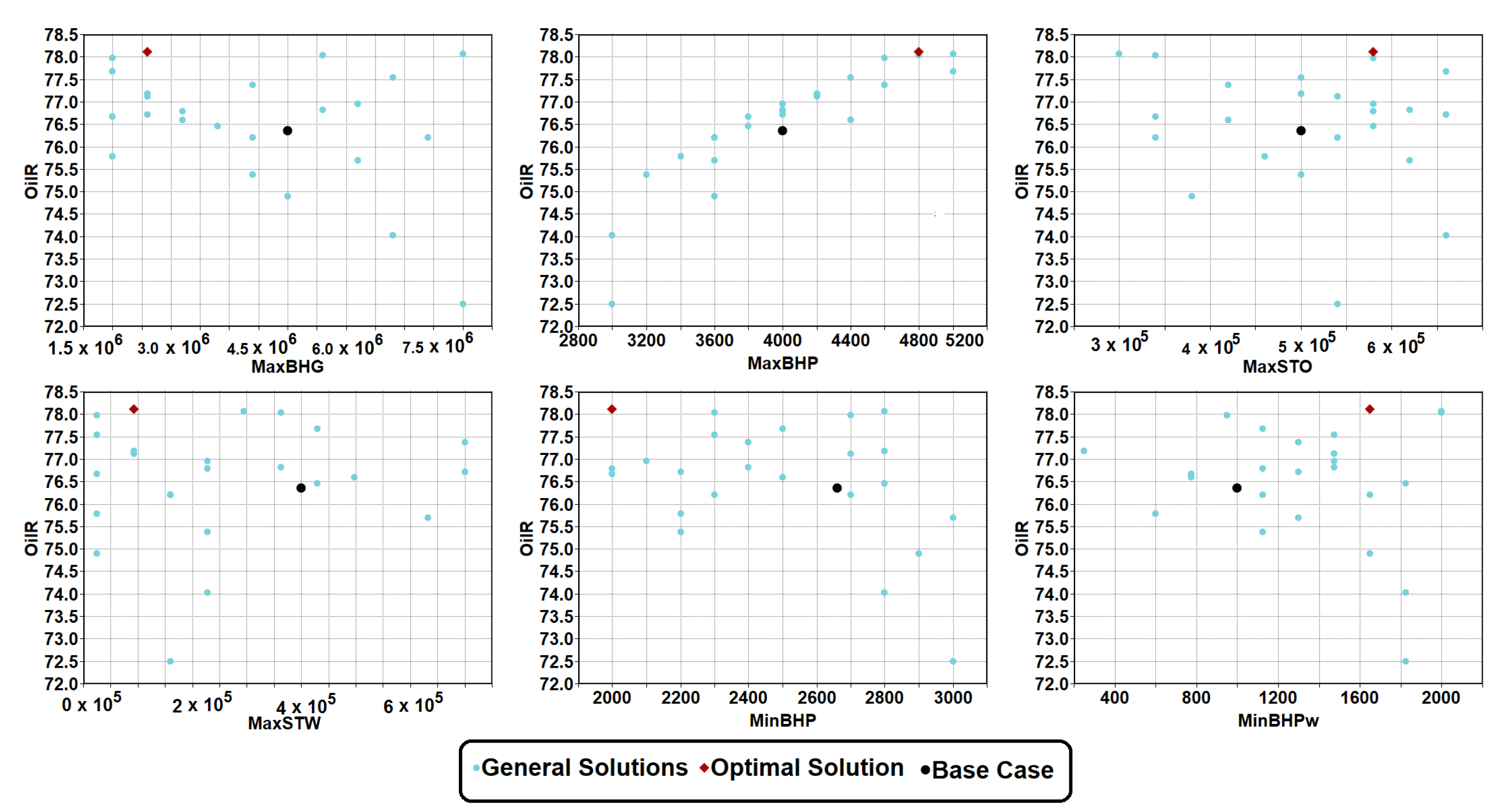
| Parameters | Min | Base Case | Max |
|---|---|---|---|
| MAXSTO, STB/DAY | 300,000 | 500,000 | 700,000 |
| MINBHP, PSI | 2000 | 2660 | 3000 |
| MAXBHG, SCF/DAY | 2,000,000 | 5,000,000 | 8,000,000 |
| MAXBHP, PSI | 3000 | 4000 | 5000 |
| MAXSTW, STB/DAY | 25,000 | 400,000 | 700,000 |
| MINBHPw, PSI | 250 | 1000 | 2000 |
| Response | Base Case | Optimal |
| Recovery factor | 76.3675% | 78.120033% |
| Parameters | Advanced Case | Optimal |
| MAXSTO, STB/DAY | 500,000 | 580,000 |
| MINBHP, Psia | 2660 | 2000 |
| MAXBHG, SCF/DAY | 5,000,000 | 2,600,000 |
| MAXBHP, Psia | 4000 | 4800 |
| MAXSTW, STB/DAY | 400,000 | 92,500 |
| MINBHPw, Psia | 1000 | 1650 |
Disclaimer/Publisher’s Note: The statements, opinions and data contained in all publications are solely those of the individual author(s) and contributor(s) and not of MDPI and/or the editor(s). MDPI and/or the editor(s) disclaim responsibility for any injury to people or property resulting from any ideas, methods, instructions or products referred to in the content. |
© 2024 by the authors. Licensee MDPI, Basel, Switzerland. This article is an open access article distributed under the terms and conditions of the Creative Commons Attribution (CC BY) license (https://creativecommons.org/licenses/by/4.0/).
Share and Cite
Al-Mudhafar, W.J.; Rao, D.N.; Wojtanowicz, A.K. Leveraging Designed Simulations and Machine Learning to Develop a Surrogate Model for Optimizing the Gas–Downhole Water Sink–Assisted Gravity Drainage (GDWS-AGD) Process to Improve Clean Oil Production. Processes 2024, 12, 1174. https://doi.org/10.3390/pr12061174
Al-Mudhafar WJ, Rao DN, Wojtanowicz AK. Leveraging Designed Simulations and Machine Learning to Develop a Surrogate Model for Optimizing the Gas–Downhole Water Sink–Assisted Gravity Drainage (GDWS-AGD) Process to Improve Clean Oil Production. Processes. 2024; 12(6):1174. https://doi.org/10.3390/pr12061174
Chicago/Turabian StyleAl-Mudhafar, Watheq J., Dandina N. Rao, and Andrew K. Wojtanowicz. 2024. "Leveraging Designed Simulations and Machine Learning to Develop a Surrogate Model for Optimizing the Gas–Downhole Water Sink–Assisted Gravity Drainage (GDWS-AGD) Process to Improve Clean Oil Production" Processes 12, no. 6: 1174. https://doi.org/10.3390/pr12061174