Simulation of Elbow Erosion of Gas–Liquid–Solid Three-Phase Shale Gas Gathering Pipeline Based on CFD-DEM

Abstract

Shale gas gathering pipelines often contain liquid water and solid sand in the early stage of production, which leads to the failure of pipeline components easily under the action of gas–liquid–solid three phases. A computational fluid dynamics (CFD) model based on the fluid volume method (VOF) and discrete element method (DEM) was established to study the flow law of gas–liquid–solid three-phase flow in the elbow of shale gas gathering pipeline and the erosion law of the inner surface of the elbow was studied by coupling the Oka erosion prediction model. By comparing the experimental results of erosion damage of the elbow, it is found that the model established can well predict the erosion characteristics and erosion amount under the action of three phases. Combined with the field pipeline parameters and operating conditions, the paper further simulates the elbow erosion behavior under relevant working conditions. The results show that the particles rotate clockwise from the outer wall of the pipe through the bottom of the pipe when passing through the elbow under the action of gas and water phases. When the gas velocity increases, the particles at the elbow mainly gather at the bottom of the elbow and the wall of the outer arch. When the water content increases gradually, the particles gathered on the outer arch wall of the elbow move along the outer arch wall of the elbow and face the inner arch surface gradually, and the erosion area is mainly concentrated on the outer arch wall of the elbow and the outlet horizontal pipe. Under the condition of the liquid phase, the movement characteristics of the water phase and particles in the elbow of the gas gathering pipeline and the erosion characteristics of the pipeline surface are obviously different from those under the condition of the gas–solid two-phase. The model and simulation results established in this paper provide a reference for the erosion damage protection of shale gas gathering pipeline elbow.

1. Introduction

After the “shale gas revolution” in the United States, China, as the largest shale gas producer after North America, has also made continuous effortfs to greatly increase the effective development of shale gas, resulting in the rapid growth of shale gas production [1,2]. The shale gas revolution reshapes the global energy landscape and affects the energy strategies of various countries. However, when the shale gas carrying solid particle impurities is initially desanded from the wellhead gas extraction tree through the gas production pipeline to the high-pressure desanding sled, and then the shale gas enters the separator for gas–liquid separation and further desanding. Due to the limited mesh size (100 μm) of the desanding device and the structure of the desanding device, the liquid shale gas after the desanding device will still carry part of the sand particles. At this point, liquid, sand, and shale gas move in the shale gas gathering pipeline at high speed and impact the pipeline wall at a certain speed and angle, causing serious erosion and wear on the pipeline wall [3]. The elbow, as a part that makes the fluid flow direction change suddenly, is seriously thinned by the erosion of gas–liquid and impurities, which is very likely to cause leakage and pipe explosion accidents [4,5,6].

In recent years, to explore the mechanism and corresponding laws of multiphase flow particle erosion, many scholars have carried out different studies, especially for multiphase flow erosion with complexity and randomness. Peyman Zahedi [7] (2019) used noninvasive ultrasound technology to measure thickness loss at eight different points at the elbow joint under the condition of gas–sand and gas–liquid–sand flow and found that the maximum erosion position was about 40°–50° in the middle of the elbow joint. Wenshan Peng [8] (2020) designed an experimental device to study the sand flushing of elbows under the action of slug flow. The relationship between gas–liquid distribution, sand body movement, and erosion profile is analyzed, and the erosion mechanism is explained. It was found that the most severe erosion areas of pipe bend occurred at the axial angle of the elbows between 67.5 and 90 and at the circumferential angle of the elbows between 45 and 90. An erosion prediction method based on computational fluid dynamics (CFD) is proposed.

The CFD method is also an effective method adopted by many scholars in recent years to study the erosion mechanism [9,10,11,12]. Mazdak Parsi [10] analyzed gas–water–sand flows in horizontal–horizontal (H-H) standard bends with diameters of 76.2 mm (r/D = 1.5) using a computational fluid dynamics (CFD) model. For this structure, the slug/pseudo slug erosion is studied. In H-H bends, the greatest erosion occurs at the top of the outer wall of the elbow. Faris S. Bilal [12] studied the alternative geometry of a standard 90° elbow, where the ratio of elbow radius of curvature to pipe diameter is equal to 1.5 (r/D = 1.5). Paint erosion experiments were carried out on three 50.8 mm pipe elbows (90° elbows with a radius of curvature of 2.5D and 5D and 45° elbows with a radius of curvature of 1.5D) for water–sand and water–gas–sand flows. The Eulerian–Eulerian–Lagrangian CFD method was used to simulate the water–gas–sand three-phase flow. In CFD and experiments, good consistency was observed for the erosion mode and maximum erosion position. M. Bayareh [13] used a finite difference/front tracking method to investigate the equilibrium position of a deformable drop in Couette and Poiseuille flows. Feng [14] studied the lift on a particle that is caused by its proximity to a boundary and the equilibrium position of this particle in a linear shear flow using the lattice Boltzmann method. A. Farokhipour et al. [15] used a three-phase calculation model (VOF and Lagrange particle tracking) to analyze the sand erosion problem of gas–liquid–solid annular flow in the elbow. The results show that higher gas velocity leads to higher particle impact velocity and thus increases erosion. Sedrez et al. [16] conducted multiphase flow erosion experiments of water, air, and sand particles and simulated them using the Euler–Lagrange method and Reynolds stress model (RSM), which obtained very good consistency.

Ogunsesa [17] adopted the Eulerian Multifluid-VOF model for gas–water two-phase flow and coupled it with the Lagrange particle tracking framework. The experimental data were basically consistent, and the corrosion in the bend was observed to be more than 45°. Zhang et al. [18] used the VOF method to simulate the two-phase flow at high gas velocities and low liquid rates and conducted particle tracking at the same time to study the annular flow behavior and particle collision characteristics. The particle collision characteristics under different working conditions are compared with the experiment, which has a good consistency. The results show that the multifluid VOF method can simulate multiphase flow well, but its main limitations are instability and convergence. This paper will use the Lagrangian method for particle simulation.

In the past, the DPM model was used to simulate the erosion of particles, ignoring the actual volume of particles and collisions between particles. Therefore, more and more scholars have adopted CFD-DEM (Computational Fluid Dynamics and Discrete Element Method) [19,20,21,22,23]. This is mainly because the CFD-DEM method adopts complete discrete elements to solve and calculate particles. It not only considers the volume of particles in the fluid and adopts the actual particle model but also considers the interaction between particles and fluid and particles.

Previous studies on particle erosion have primarily focused on two-phase flow erosion, such as gas–solid and liquid–solid interactions. However, research on the erosion of gas–liquid–solid three-phase flow in 90° elbows of shale gas gathering pipelines remains limited. In this study, the VOF-DEM method was used to simulate the elbow of the shale gas gathering pipeline. Based on the field survey data, different gas–liquid–solid multiphase flow simulation conditions were designed, and different gas velocities, gathering pressure, and water content were compared to analyze the gas–liquid distribution and particle trajectory, and the erosion law of the pipe elbow was summarized. It provides theoretical support for the study of erosion and the optimization of the elbow.

2. Numerical Modeling

2.1. VOF-DEM Modeling

Due to the variable interface in gas–liquid two-phase flow, it has a more complex flow state than single-phase flow. In this paper, the VOF model [24,25] is adopted for numerical solution.

(1)

Continuity equation: Tracking the interface between phases is carried out by solving the continuity equation for the volume ratio of a single or multiphase fluid. For phase q, there is the following:

$$\frac{\partial {\alpha }_q}{\partial t}+\overrightarrow{\nu }\nabla {\alpha }_q=0$$

(1)

where α_q is volume fraction of the q phase; v is the gas velocity; and t is the time.

The volume fraction of the main phase is calculated based on the following constraints:

$${\displaystyle \sum _{q=1}^n{\alpha }_q}=1$$

(2)

(2)

Momentum equation: By solving a single momentum equation for the entire region, the resulting velocity field is shared by the phases. The momentum equation depends on the volume ratio of all phases through the properties ρ and μ. The equation is as follows:

$$\frac{\partial }{\partial t}\left(\rho \overrightarrow{\nu }\right)+\nabla \cdot \left(\rho \overrightarrow{\nu }\overrightarrow{\nu }\right)=-\nabla p+\left[\mu \left(\nabla \overrightarrow{\nu }+\nabla {\overrightarrow{\nu }}^T\right)\right]+\rho \overrightarrow{g}+\overrightarrow{F}$$

(3)

where $\rho$ is the fluid density, $p$ is the gas pressure, $\mu$ is the gas viscosity, $g$ is the acceleration of gravity, and $F$ describes the forces acting on a phase, such as surface tension.

When CFD-DEM coupling calculation of fluid and particle motion is carried out, the discrete element method in the Lagrangian coordinate system is adopted to solve solid particles. The motion equation of a single particle (i) is composed of a translational equation [26] and a rotational equation, which follows Newton’s second law of motion. When tracking the motion path of particles, the velocity and position of particles at every moment can be obtained by the external force. When particles follow fluid, the motion of each particle is affected by the surrounding fluid and adjacent particles. The translational and rotational motion of particles are calculated according to Newton’s second law [26], given by the following:

$$m_{p,i}\frac{\mathrm{d}{u}_{p,i}}{\mathrm{d}t}={\displaystyle \sum F_{pc,ij}}+F_{lp,i}+m_{p,i}g$$

(4)

$$I_{pc,ij}\frac{\mathrm{d}{\omega }_{p,i}}{\mathrm{d}t}=T_{pc,ij}$$

(5)

where m_i is the mass of particle i, u_p,i is the linear velocity of particle i; F_pc,ij is the contact force of particle i in contact with other particles, $F_{lp,i}$ is the fluid force on particle i, $I_{pc,ij}$ is the moment of inertia of particle i, ${\omega }_{p,i}$ is the angular velocity of particle i, and $T_{pc,ij}$ is the contact torque resulting from particle i contacting particle j.

2.2. Turbulence Model

The standard k-ε turbulence model is used at the turbulence core due to its suitability for turbulent flows with large Reynolds numbers, and the standard wall function is used in the near-wall area. The widely used Standard k-ε turbulence model is described by the turbulent kinetic energy k equation and turbulent dissipation rate ε equation [27].

The turbulent viscosity μ_t is computed by combining k and ε as follows:

$${\mu }_t=\rho C_{\mu }\frac{k^2}{\epsilon }$$

(6)

where C_μ is 0.09.

In the standard k-ε turbulence model, the transport equations of k and ε are as follows:

$$\frac{\partial \left(\rho k\right)}{\partial t}+\frac{\partial \left(\rho k{u}_i\right)}{\partial x_i}=\frac{\partial }{\partial x_j}\left[\left(\mu +\frac{{\mu }_t}{{\sigma }_k}\right)\frac{\partial k}{\partial x_j}\right]+G_k+G_b-\rho \epsilon -Y_M+S_k$$

(7)

$$\frac{\partial \left(\rho \epsilon \right)}{\partial t}+\frac{\partial \left(\rho \epsilon u_i\right)}{\partial x_i}=\frac{\partial }{\partial x_j}\left[\left(\mu +\frac{{\mu }_t}{{\sigma }_{\epsilon }}\right)\frac{\partial \epsilon }{\partial x_j}\right]+C_{1\epsilon }\frac{\epsilon }{k}(G_k+C_{3\epsilon }{G}_b)-C_{2\epsilon }\rho \frac{{\epsilon }^2}{k}+S_{\epsilon }$$

(8)

where k is the turbulent kinetic energy, m²/s²; ε is the turbulent dissipation rate; μ is the gas viscosity; G_k is the turbulent kinetic energy generating term; C_1ε, C_2ε, σ_k and σ_ε are constants, and C_1ε = 1.92, C_2ε = 1.4, σ_k = 1.0, and σ_ε = 1.3.

2.3. Fluid–Particle Force

In solid–liquid–gas multiphase flow, particles are subjected to drag force, buoyancy force, pressure gradient force, virtual mass force, Saffman lift force, Basset force, Magnus force, and other forces [28]. In this paper, the buoyancy force, drag force, virtual mass force, Saffman lift force, and pressure gradient force are considered.

2.4. Erosion Prediction Model

In reference [29], the simulation results of pipeline erosion were compared with the experimental results, and the Oka model simulation results were found to be the most consistent with the experimental results. The Oka model is appropriate for erosive wear involving carbon steel target material and quartz sand grains. So, the Oka model was adopted. In the Oka model, the erosion rate was determined as follows [30,31]:

$$E=E_{90}{\left(\frac{V}{V_{ref}}\right)}^{k_2}{\left(\frac{d}{d_{ref}}\right)}^{k_3}f\left(\gamma \right)$$

(9)

where E₉₀ is the reference erosion rate at 90°, V is the particle impact velocity, V_ref is the relative velocity, d and d_ref are the particle diameter and particle reference diameter, and f(γ) is the ratio of erosion damage at arbitrary angles expressed by the two trigonometric functions and by initial material hardness number H_v, as shown in Equation (10):

$$f\left(\gamma \right)={\left(\sin \gamma \right)}^{n_1}{\left(1+H_v\left(1-\sin \gamma \right)\right)}^{n_2}$$

(10)

where γ is the wall impact angle, H_v is the wall material Vickers hardness, n₁ and n₂ is the angle function constant, expressed as a function of initial material hardness:

$$n_1=s_1{\left(H_v\right)}^{q_1},n_2=s_2{\left(H_v\right)}^{q_2}$$

(11)

where s and q are, therefore, constants, which are determined only by the type, shape, and property of particles. For quartz sand, s₁ = 0.71, q₁ = 0.14, s₂ = 2.4, and q₂ = −0.94.

3. Physical Model and Solution Method

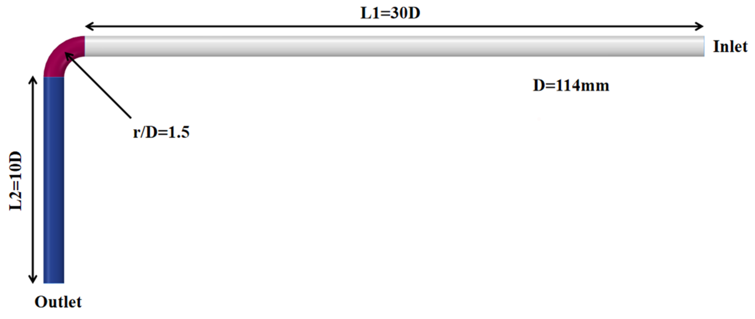
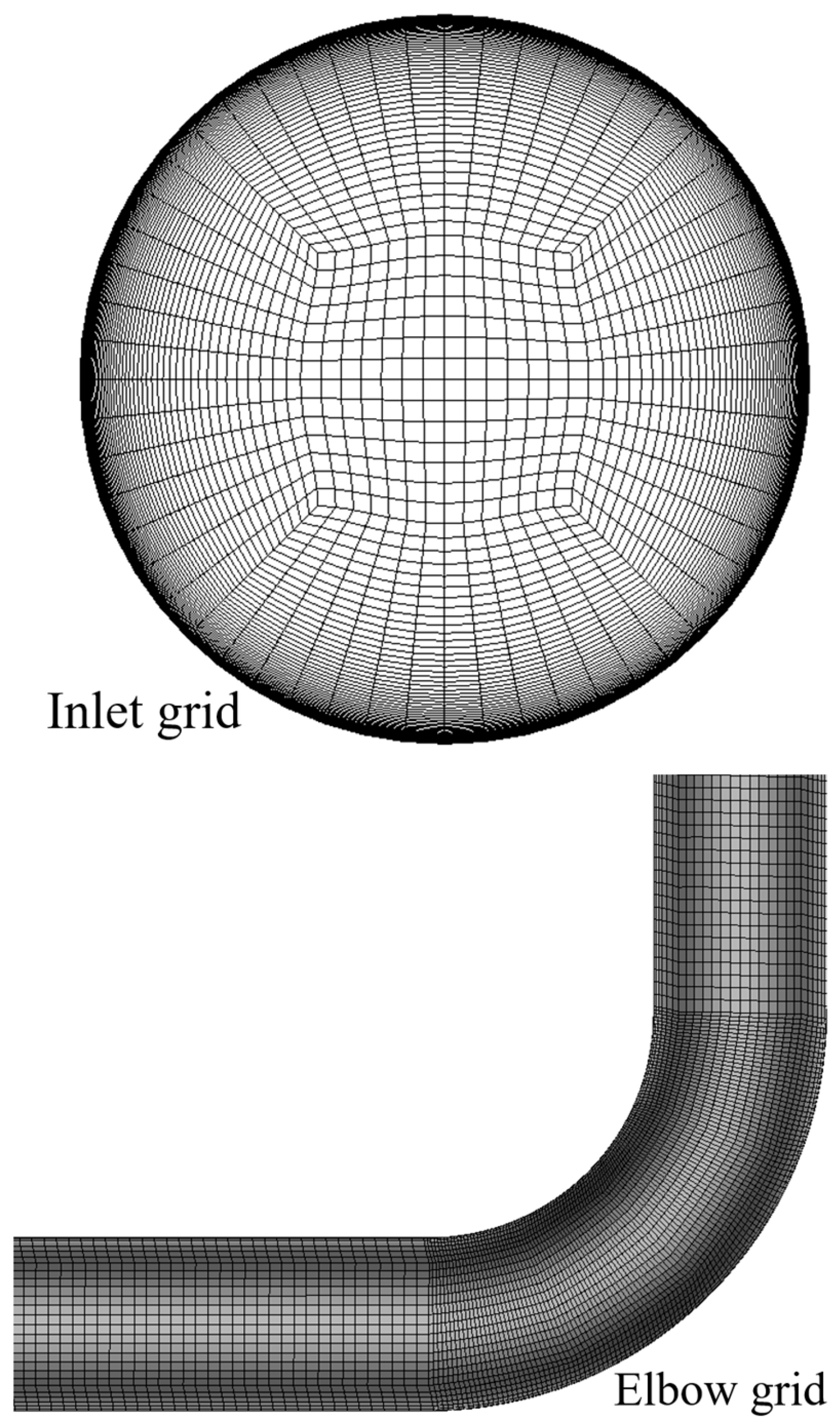
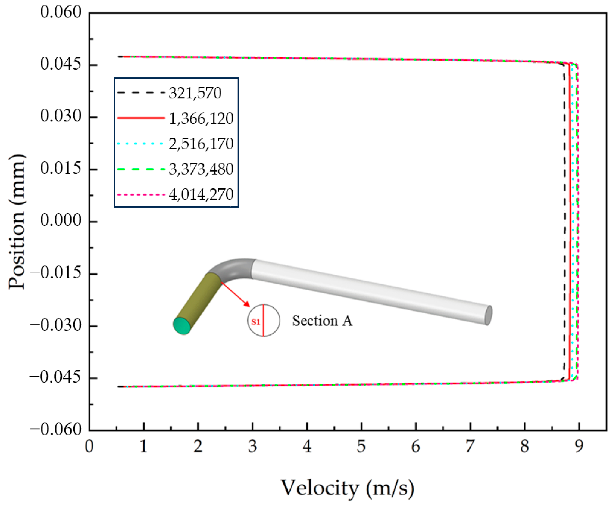
3.1. Geometry and Meshing

To ensure that the fluid and particles at the inlet of the pipeline meet the actual flow field condition when entering the elbow, the length of the horizontal straight pipe at the inlet section of the model is increased appropriately. Therefore, the geometric model can be simplified into three parts: two straight pipe sections of different lengths and a bend. The fluid domain of the whole numerical simulation study can be determined as a three-dimensional flow channel composed of two horizontal tubes and an elbow. The simplified geometric model is shown in Figure 1. Among them, diameter D = 114 mm, L1 = 30 D = 3420 mm, L2 = 10 D = 1140 mm, elbow curvature radius R = 1.5 D = 171 mm, and elbow angle is 90°. The fluid phase and particle phase enter from the entrance of the L1 section, pass through the elbow position, particle phase, and fluid phase, impact the pipe wall at the same time, and flow out from the outlet of the L2 section.

To ensure the accuracy of flow field simulation, the meshing at the inlet close to the wall and the meshing at the pipe bend are refined, respectively, and the boundary layer grid yplus is in the logarithmic region, as shown in Figure 2. The minimum mesh quality is 0.75, and the minimum angle is greater than 54° since the comprehensive quality meets the calculation requirements.

Aiming at the geometric model in Figure 1, five structured grids with the numbers 321570, 1366120, 2516170, 3373480, and 4014270 were divided by changing the number of nodes. Under the same parameters and the fluid velocity at the inlet, the velocity value at S1 in the figure was extracted. By comparing the speed values under a different number of grids, as shown in Figure 3, to consider calculation accuracy and efficiency, the grid with 3373480 grids was selected as the final calculation mesh in this paper.

3.2. Simulation Parameter Settings

3.2.1. Basic Working Condition Parameter Setting

Based on the field production investigation of shale gas fields in Changning–Weiyuan block, Sichuan Basin, China, this paper selects the production data of six wells at the early stage of production, as shown in

Table 1. Field conditions.

Well Number	Daily Gas (104 m3/d)	Pressure (MPa)	Sand Rate (kg/d)	Sand Size (mesh)
Well 1	21.6085	5.81	2.3	70~180 mesh
Well 2	21.6706	7.06	3.1	70~180 mesh
Well 3	37.9431	6.12	4.8	70~180 mesh
Well 4	44.0585	8.17	6.1	70~180 mesh
Well 5	50.3707	5.84	6.9	70~180 mesh
Well 6	62.2861	9.34	8.5	70~180 mesh

. As can be seen from the table below, the daily gas range from well 1 to well 6 ranges from 216,085 m³/d to 6222.861 m³/d, the transmission pressure is from 5.81 MPa to 9.34 MPa, the sand rate is from 2.3 kg/d to 8.5 kg/d, and the particle size is 70~180 mesh.

Based on field production investigation, the gas flow rate v = 9 m/s, gathering pressure p = 5 MPa, particle size DP = 0.105 mm, sand rate m_p = 5 kg/d, and water content 5% were selected as the reference conditions. The specific simulation conditions are shown in

Table 2. Simulation condition settings.

Influencing Factors	Specific Parameters
Gas Flow Rate (m/s)	5, 7, 9, 11
Pressure (MPa)	4, 5, 6, 7, 8, 9
Moisture Content (%)	1, 3, 5, 7

. Considering that water and gas enter from the inlet of the pipe at the same time, in this study, to fully ensure the formation of a certain amount of water in the pipe, particles can be injected only after the gas and water enter the inlet for 2 s and the gas–liquid phase reaches the equilibrium condition.

3.2.2. Particle Parameter Settings

After investigation [32], the material of sand in the pipe is basically quartz sand, and the specific parameter settings of particles are shown in

Table 3. Sand simulation parameters.

Coefficient of Restitution	Static Friction Coefficient	Rolling Friction Coefficient	Sand Density (kg/m3)	Poisson’s Ratio	Shear Modulus (Pa)
0.9	0.1	0.005	2650	0.12	2.37 × 109

. The spherical model of the sand particle was used. The normal and tangent coefficients of restitution are both 0.9.

3.3. Boundary Conditions and Simulation Procedure

The right side of section L1 is the inlet of the fluid phase and particle phase, and the boundary condition is set as the velocity inlet. The value is determined according to the actual field survey data. The left side of section L2 is the outlet of the fluid phase and particle phase, and the outlet condition is set as the pressure outlet. The pipe surface is set as static and no-slip wall boundary conditions.

Because the erosion behavior of the elbow of the shale gas gathering pipeline is a transient problem, this paper adopts the transient solver based on pressure, discretizes the flow control equation of fluid through the finite volume method, solves the equation with the SIMPLE algorithm. The calculations were conducted using the commercial software FLUENT v2019 R2 and EDEM v2018.2. The first-order implicit format is used to discretize the time domain, the unit-based least square method is used to discretize the pressure gradient equation, the second-order upwind format is used to discretize the momentum equation and volume coefficient, and the first-order upwind format is used to discretize the turbulent kinetic energy and turbulent dissipation rate. Finally, the discrete element method is used to solve the motion equation of particles to complete the final simulation process solution.

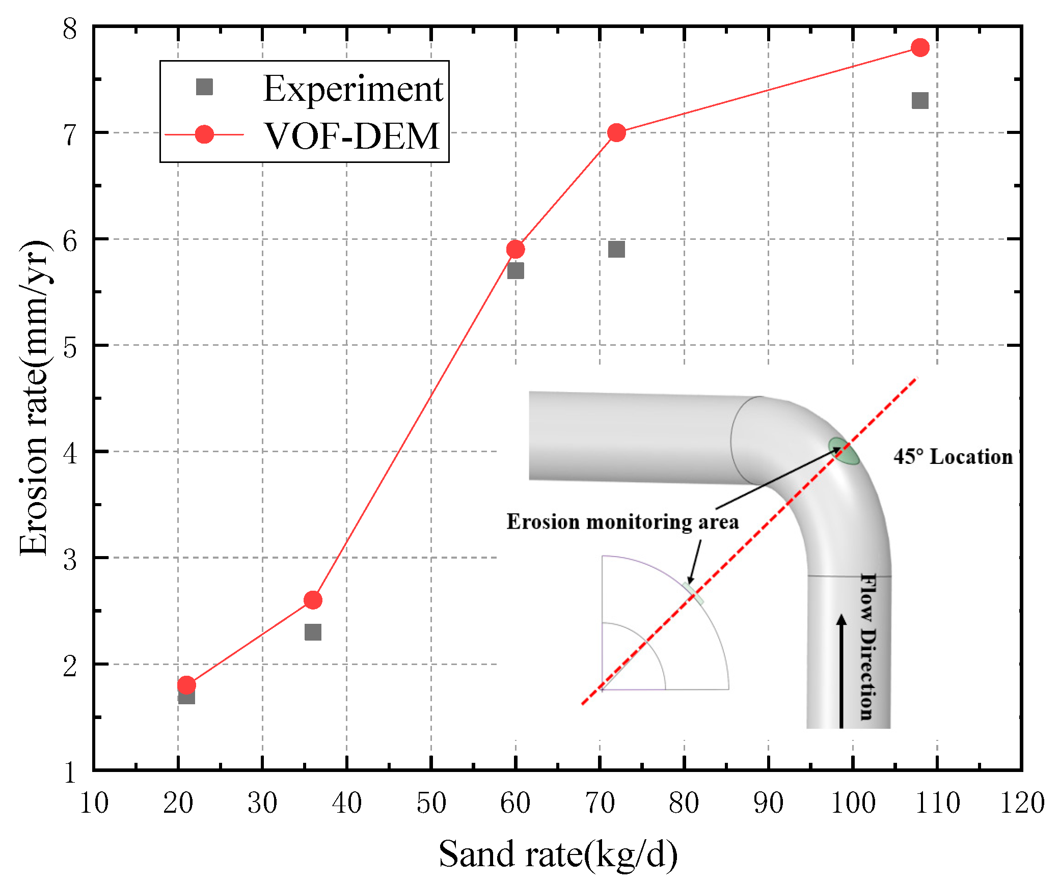
3.4. Model Validation

To test the impact of the erosion of gas–liquid–solid three-phase pipeline elbow calculated by CFD-DEM coupling simulation, the experiment was compared with the gas–liquid–solid three-phase flow erosion experiment conducted by Vieira et al. [4]. In the experiment, 316 steel was used in the elbow wall, the inner diameter was 76.2 mm, the radius of curvature was 1.5, and the probe was installed at 45° of the elbow. The sand particle size is 300 microns, gas velocity is 27 m/s, and apparent liquid velocity is 0.005 m/s, 0.009 m/s, 0.015 m/s, 0.018 m/s, and 0.027 m/s. Multiphase flow erosion simulation was carried out under the same experimental conditions, and the simulation results are shown in Figure 4. The error at the elbow outlet is relatively large, likely due to discrepancies between the model and actual pipeline turbulence in capturing turbulent motion. However, the differences at other locations are minimal and meet the calculation requirements.

4. Results and Discussion

4.1. Three-Phase Flow Characteristic

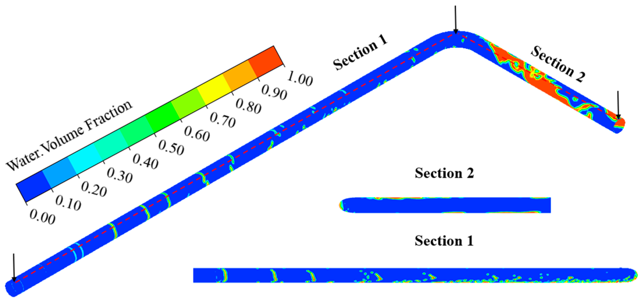
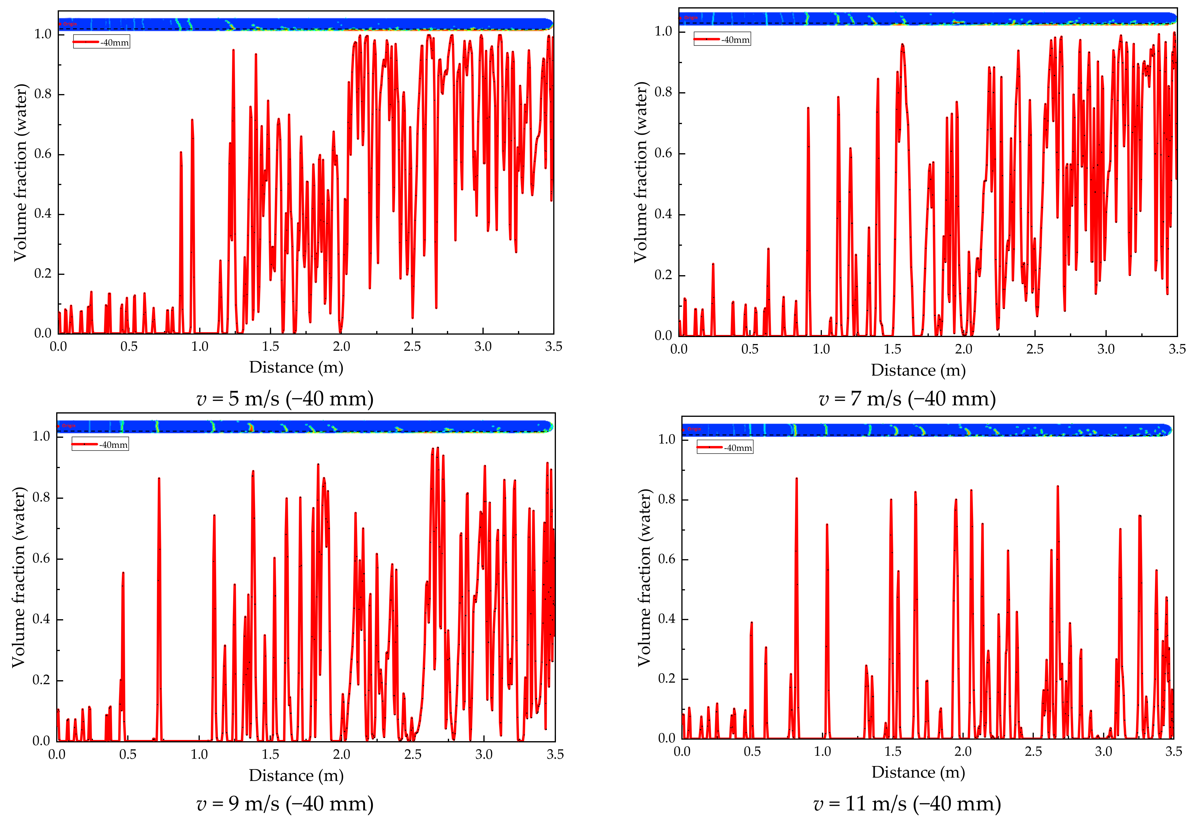
4.1.1. Analysis of Gas–Liquid Two-Phase Flow

The first is the analysis of the change in gas velocity. In this study, the gas inlet velocity is set to be consistent with the particle velocity. When the gas velocity increases, the particle velocity increases synchronically, and the erosion wear on the pipe wall will be more severe. Figure 5 shows the gas–liquid distribution diagram of the basic working condition, where Sections 1 and 2 are the sections of the two axes of the pipeline, respectively. Figure 6 shows the water phase content at the bottom of the pipe −40 mm away from the origin. When the gas velocity increases from 5 m/s to 9 m/s, there is a certain amount of water at the bottom of Section 1. When the gas velocity increases, the water at the bottom of the section gradually diffuses into the gas; that is, the water at the bottom of the horizontal pipe at the entrance of the pipe gradually decreases with the increase in the gas velocity. In addition, it can be seen that there is basically no water at the bottom of Section 2 and a certain amount of diffuse water phase at the top. When the gas flow rate is 11 m/s, due to the large flow rate, the volume of water at the bottom of Section 1 is small, and there is a water phase dispersed in the gas near the bottom of the pipe, while the water phase at Section 2 exists at the top of the section. At the same time, the gas–liquid phase enters from the inlet of the pipe, and after passing through the elbow, the liquid phase flows along the top of the pipe to the outlet section. To sum up, when the gas flow rate is small, the velocity of the water phase is small, the drag force of gas on the water phase is small, and a certain amount of water is formed in the horizontal section of the pipeline entrance. When the gas velocity increases, the water phase velocity increases, and the force of the gas phase on the water phase increases, so stable water cannot be formed. The amount of water is small, and some water phases are dispersed. When the flow continues, after the water phase passes through the elbow, due to the joint action of inertia and gas phase, the water phase flows along the top of the pipe to the outlet of the pipe, and the larger the gas flow rate, the farther the water phase flows along the top of the pipe.

The change in gathering pressure in the gas gathering pipe has the greatest influence on gas flow in the pipe. When the gas flow changes, the water phase and particles in the tube affected by the gas will also be affected to a certain extent. As can be seen from the main view of Figure 5, an intermittent annular water phase exists on the horizontal pipe wall of the inlet section of the pipeline, and a large amount of water phase exists on the top of the horizontal pipe wall of the outlet section. With the increase in gathering pressure, the water phase gradually transforms from an aggregation state to a dispersed state. At the same time, the higher the gathering pressure is, the closer the water phase at the top of the outlet section is to the pipe outlet. This is because the higher the gathering pressure is, the greater the gas drag force of the water phase is, and the faster the water phase flows, the closer it is to the pipe outlet. When the gathering pressure is 5~6 MPa, there is a small amount of water at the bottom of the inlet section of the pipeline. When the gathering pressure continues to increase, the water at the bottom of the pipeline gradually disperses into the gas in the pipe. When the gathering pressure is 5–7 MPa, there is water at the bottom of the outlet section of the pipeline. When the gathering pressure continues to increase, the water at the bottom of the outlet section of the pipeline decreases. In summary, with the increase in gathering pressure, the water volume at the bottom of the inlet pipe decreases, while the water phase at the top of the outlet pipe gradually changes from the state of aggregation to the state of dispersion, and the greater the pressure, the closer the water phase is to the outlet of the pipe (Figure 7).

When the water content in the pipe is 1%, there is less water at the top of the horizontal pipe at the outlet end, and there is basically no water at the bottom of Sections 1 and 2, while a small amount of water exists at the top of Section 2. When the water content in the pipe is 3%, 5%, and 7%, the water phase content at the top of the horizontal pipe in the outlet section increases gradually, and the water at the bottom of Section 1 increases gradually (Figure 8).

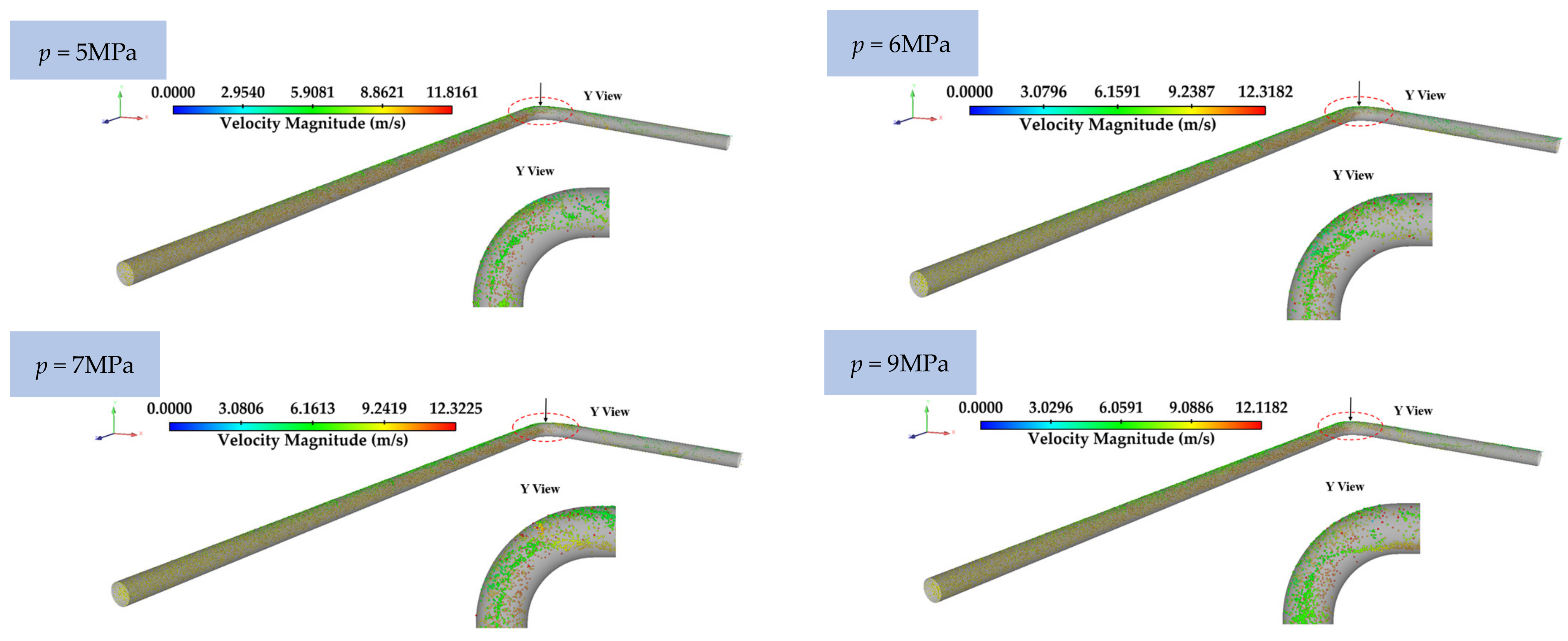
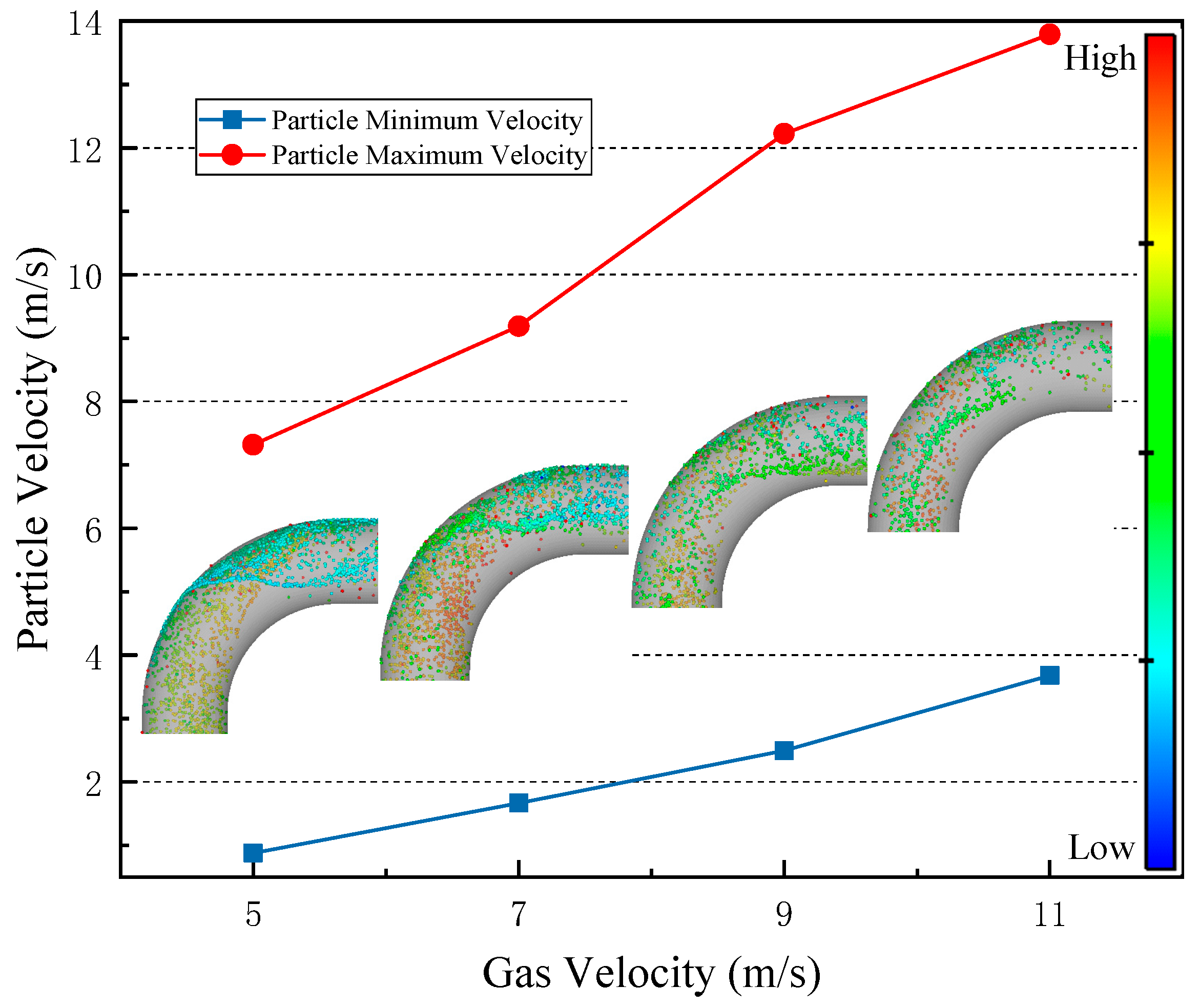
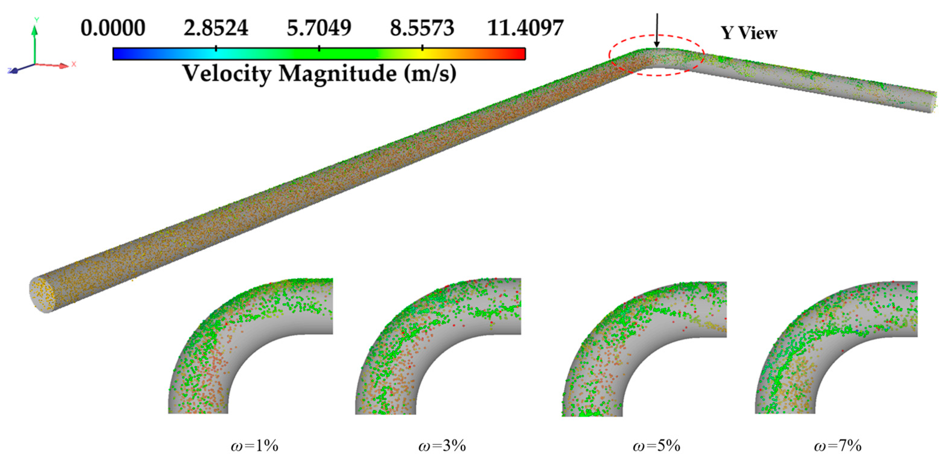
4.1.2. Particle Velocity Distribution and Trajectory

As can be seen from the main view of Figure 9, the velocity distribution of particles in the inlet pipe is different. The velocity in the middle of the pipe is larger, while the velocity near the top of the pipe is smaller. When passing through the elbow, particles move close to the outer arch wall of the elbow, and the velocity decreases. From Y view, when the gathering pressure is 5–6 MPa and the flow time is 4.5 s, most particles gather on the outer arch wall of the elbow. When the gathering pressure increases from 6 MPa to 9 MPa, the particles on the outer arch wall disperse gradually and move toward the inner arch surface. The analysis shows that as the gathering pressure increases, the overall force of particles increases, and the particles move clockwise along the wall to the top of the wall before passing through the elbow, which is consistent with the characteristics of particles moving toward the inner arch wall in Y view.

As shown in Figure 10, particles enter from the inlet of the pipe at different velocities, and the velocity decreases when passing through the elbow, and the particle velocity near the outer arch wall of the elbow is the smallest. After passing through the elbow, the potential energy of particles is converted into kinetic energy, and the particle velocity continues to increase until it flows out of the pipe under the action of the gas. At the same time, with the increase in gas velocity, the number of particles at the elbow gradually decreases. This is because the particle velocity increases synchronously with the gas velocity, and the particles pass through the elbow quickly, making the number of particles in the elbow small at the moment. It can be seen that the maximum velocity of particles in the pipeline increases synchronously with the increase in gas velocity.

As can be seen from the local enlarged figure in Figure 11, when the water content in the pipe is 1%, the particles mainly gather on the outer arch wall of the elbow. When the water content in the pipe increases gradually, the particles gathered on the outer arch wall of the elbow gradually disperse to the inner arch wall of the elbow.

Gas–liquid–solid three-phase flow through the elbow in the trajectories of particles, as shown in Figure 12, the particles from the entrance into the pipeline, along the bottom of the pipe to elbow movement, through the elbow particle collision with bend arch wall outside, and then from outside bend arch wall along the pipe at the top of the spiral movement to the bottom of the pipeline, the flow from exports, under different water content, gas velocity, and gas gathering pressure. The trend of particle movement remains unchanged.

4.2. Analysis of Elbow Erosion

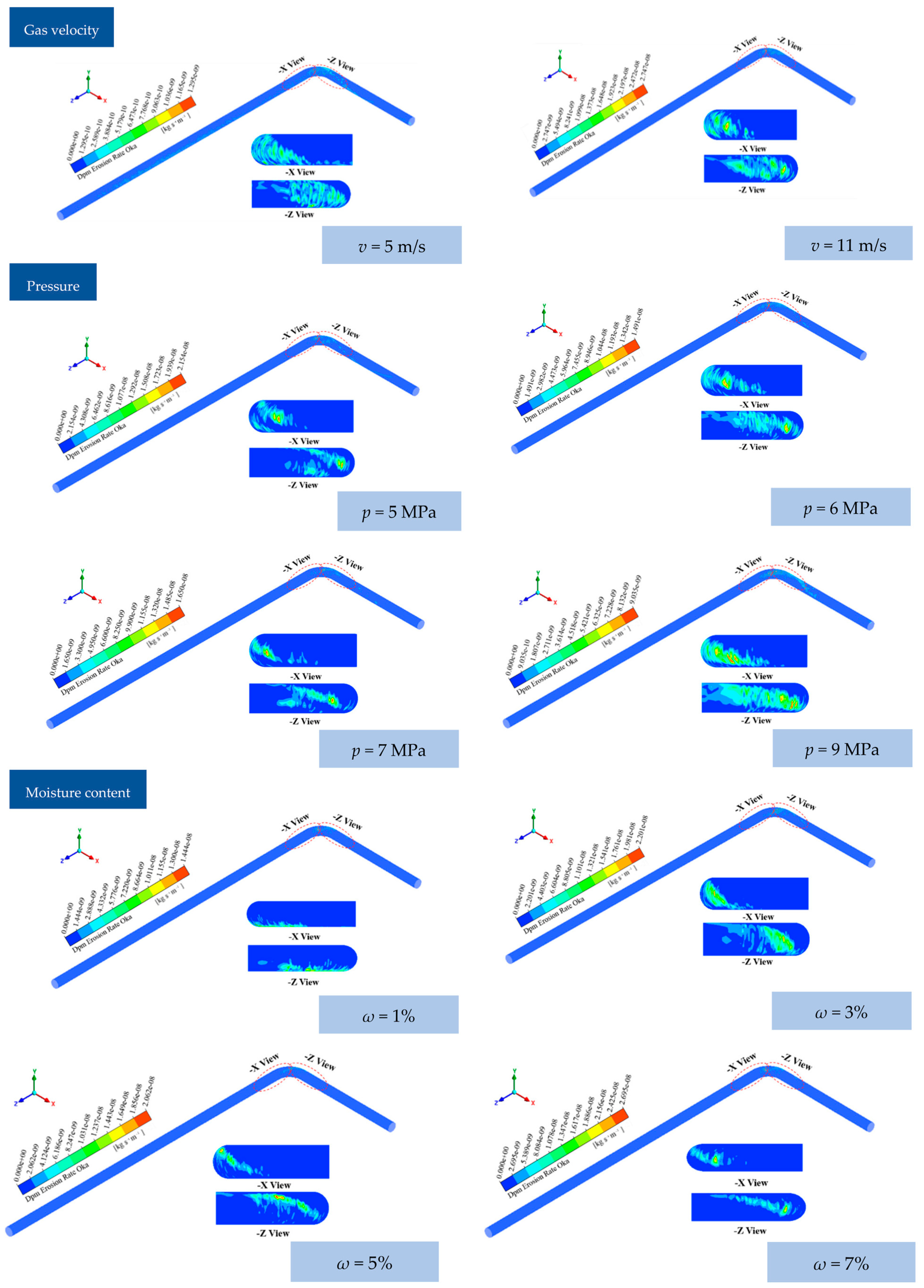
4.2.1. Elbow Wall Erosion

It can be seen from Figure 13 that when the gas flow rate changes, the serious erosion of the elbow is on the outer arch wall of the elbow. The analysis shows that the higher the gas velocity, the higher the particle velocity, the greater the kinetic energy, resulting in the more intense collision between particles and the wall, the more serious the wall erosion. At the same time, with the increase in particle velocity, more energy particles can be converted into the outer arch wall of the elbow, and the position of serious erosion of the wall will gradually shift to the middle and upper part of the outer arch wall.

When the gathering pressure changes, the erosion position at the elbow of the pipeline is consistent with the collision contact position between the particles passing through the elbow and the elbow in the upper section, that is, the position of the outer arch wall of the elbow near the top of the pipeline. When the gathering pressure is 5~7 MPa, the erosion position of the elbow is concentrated on the outer arch wall of the elbow directly opposite the entrance. When the gathering pressure is 9 MPa, the erosion area includes all areas eroded under the above pressure conditions. The analysis shows that when the gathering pressure is small, the serious erosion position of the elbow is mainly where the particles collide with the elbow wall for the first time. When the gathering pressure increases, the particles are affected by the drag force of gas, and the collision with the elbow becomes more intense, resulting in erosion wear at all positions where the particles come into contact with the elbow wall, so the erosion area on the wall increases.

When the water content in the pipe is 1%, the serious erosion position of the elbow is at the bottom of the outer arch wall. When the water content in the pipe is 3%, the serious erosion position of the elbow shifts from the bottom of the outer arch wall to the middle and upper part, and the erosion area is large. When the water content in the pipe is 5%, the serious erosion position of the elbow continues to shift to the top, and the erosion area decreases. When the water content in the pipe is 7%, the serious erosion position of the elbow shifts to the middle of the outer arch wall, and the erosion area continues to decrease. The analysis shows that when the water content in the pipe is low, the water phase is not evenly distributed in the pipe, and no water is formed, which changes the normal movement track of particles passing through the elbow, making particles pass through the elbow from the bottom of the pipe, so the erosion position caused to the wall is at the bottom of the pipe. When the water content in the pipe increases, the water content of the water phase increases, and the water phase flows in the pipe to promote the normal movement of particles so that the erosion position of the elbow moves from the outer arch wall of the elbow to the top of the pipe. When the water content in the tube continues to increase, the water phase reduces the collision area between particles and the wall surface, and the erosion area relatively decreases.

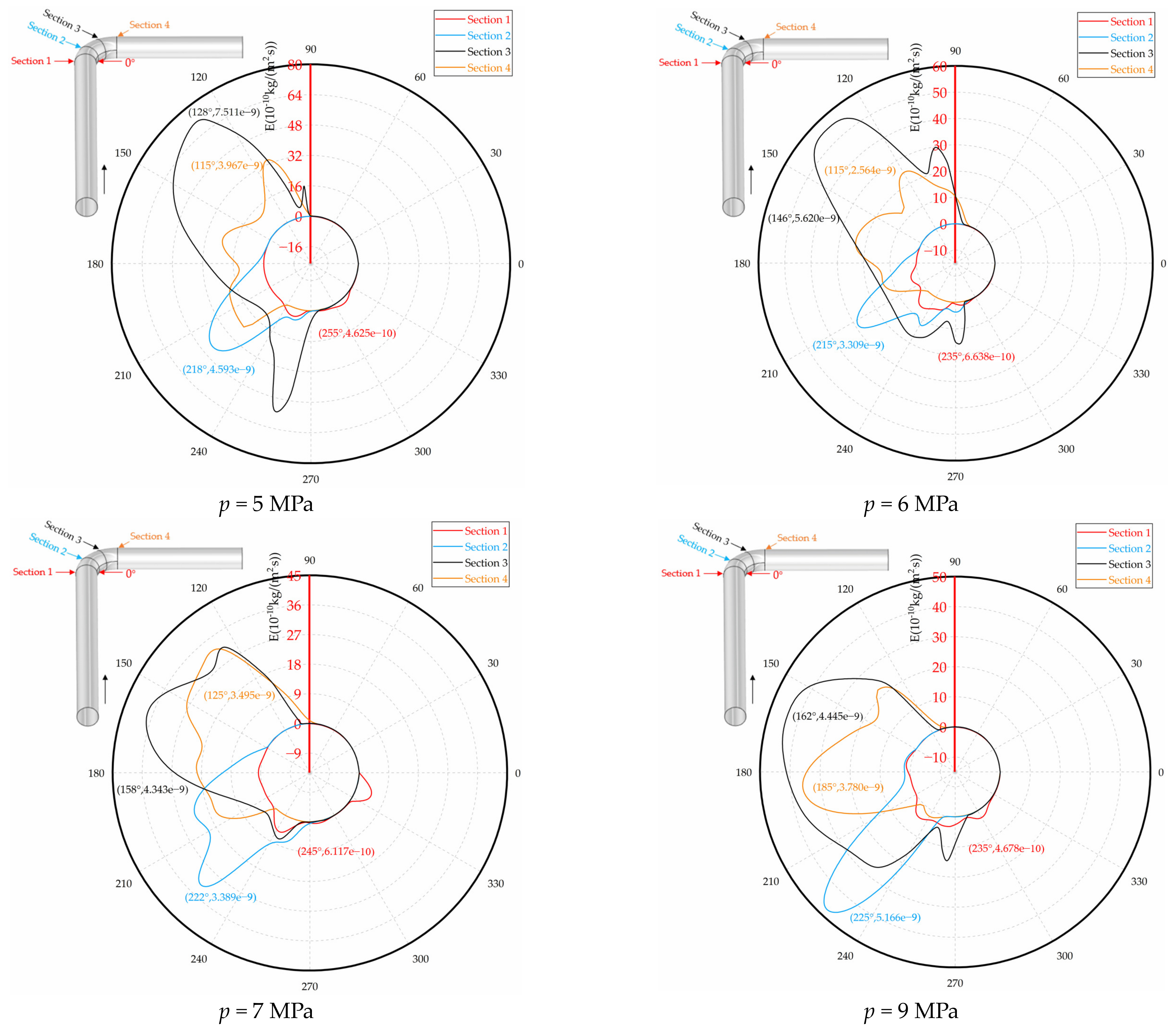
4.2.2. Circumferential Erosion of Elbow

The research object of this study is mainly the elbows of the gas gathering pipeline. To study the erosion positions and erosion rates of elbows on the upper wall of different sections, the elbows of the pipeline are divided into four sections, namely Section 1, Section 2, Section 3, and Section 4, corresponding to the four positions from the elbow inlet to the elbow outlet, as shown in Figure 14.

As can be seen from Figure 14, when the gas flow rate is constant, the erosion area of the elbow wall from Section 1 to Section 4 rotates clockwise. When the gas flow rate gradually increases, the erosion area from Section 1 to Section 4 rotates clockwise from the outer arch wall of the elbow to the top of the pipe. In conclusion, the erosion positions in the same section are basically the same under different gas flow rates. The greater the gas velocity, the greater the erosion degree of the same section of the elbow.

Figure 15 shows that when the gathering pressure is constant, the erosion area of the elbow wall from Section 1 to Section 4 rotates clockwise along the pipeline. At the same time, with the increase in gathering pressure, the maximum erosion rate in Section 3 is the largest. In summary, the erosion position of the elbow wall shifts clockwise along the pipeline with the movement direction of particles, and the most serious erosion area of the elbow is near Section 3. At the same time, near Section 3, the collision between particles and the elbow is the most intense, so the erosion is the most serious.

According to Figure 16, when the water content of the pipe is constant, the erosion area of the elbow wall from Sections 1 to 4 rotates clockwise from the outer arch wall of the elbow along the top of the pipe. With the increase in water content in the pipe, the maximum erosion at the elbow is at Section 3, and with the increase in water content, the maximum erosion position at Section 3 rotates slowly clockwise. In summary, the erosion position of the elbow wall shifts clockwise along the pipeline with the direction of particle movement. When the water phase in the tube increases, the particles are affected by the resistance of the water phase, which causes large erosion wear at the position where the particles collide with the elbow directly; that is, the erosion at Section 3 is more serious (Figure 16).

5. Conclusions

A gas–liquid–solid three-phase coupled flow model based on the VOF-DEM method was established to study erosion behavior in gas gathering pipeline elbows. For the results, the following conclusions can be made:

(1)

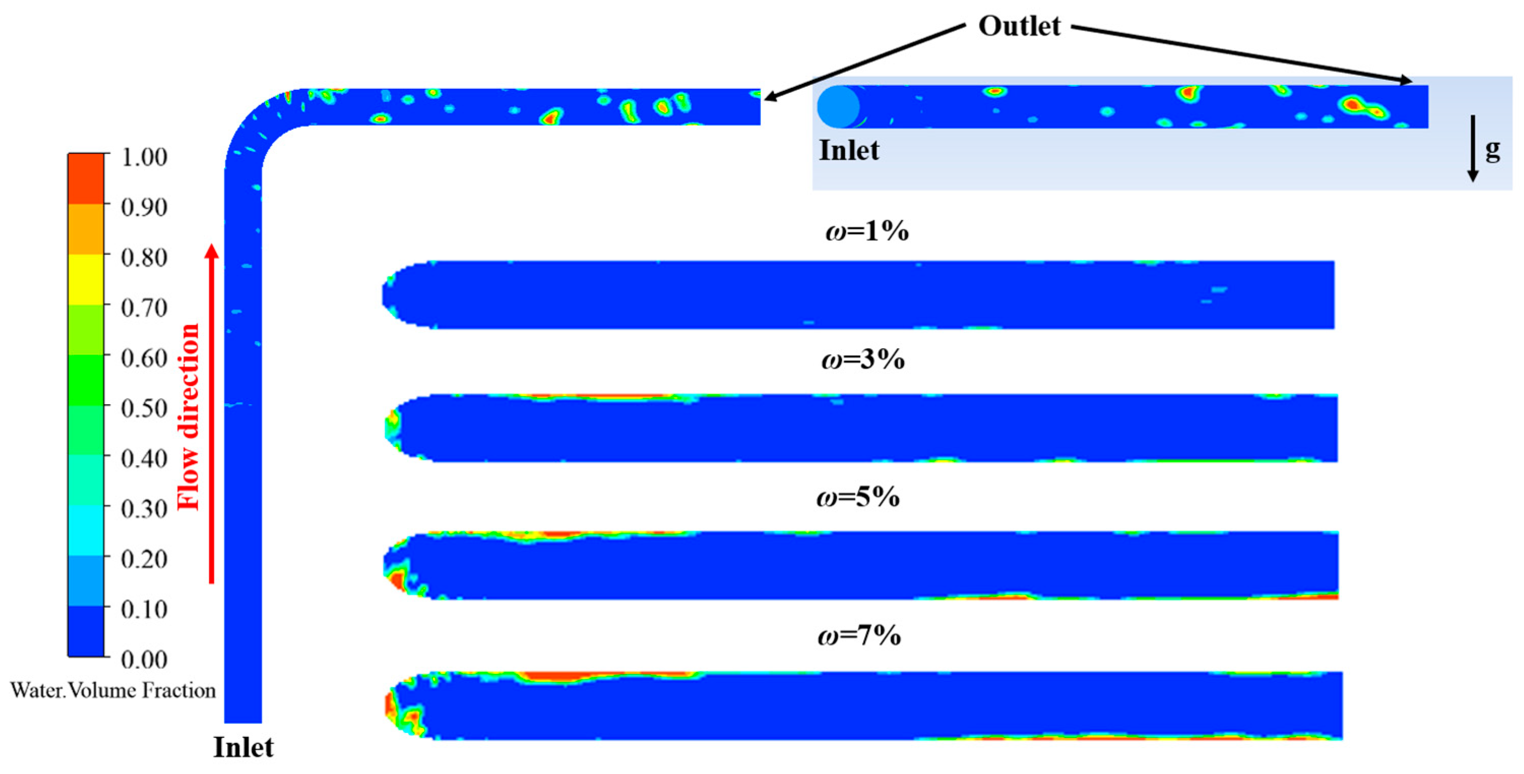
When the gas flow rate is small, there is a certain amount of ponding at the bottom of the inlet pipe. When the gas flow rate increases, the volume of water in the horizontal section of the inlet is small and some water phase is dispersed. When the gathering pressure is small, there is a certain amount of ponding at the bottom of the inlet pipe. With the increase in gathering pressure, the water volume at the bottom of the inlet pipe decreases, while the water phase at the top of the outlet pipe changes from the state of aggregation to the state of dispersion. When the water content in the pipe is small, there is basically no ponding at the bottom of the inlet pipe. When the water content increases, the volume of water in the tube increases, and the height of the water increases. The water phase at the elbow mainly collects on the outer arch wall and the top area of the elbow outlet.

(2)

When the gas flow rate, gathering pressure, and water content in the pipe change, respectively, the particles move from the bottom of the pipe to the elbow after entering the inlet pipe and then collide with the outer arch wall of the elbow and rotate counterclockwise along the outer arch wall of the outlet pipe facing the top of the pipe. At the same time, the erosion area of the elbow is consistent with the movement track of particles at the elbow, mainly concentrated on the outer arch wall of the elbow and the inclined area between the outer arch wall of the elbow and the top of the outlet pipe.

(3)

When the gas flow rate increases, the particles at the elbow mainly gather at the bottom of the elbow and the outer wall, and the maximum particle velocity increases with the increase in the gas flow rate. When the gathering pressure is 4–8 MPa, most of the particles mainly collect at the bottom of the pipeline and the outer arch wall, and when the gathering pressure increases to 9 MPa, the particles gradually move to the top of the outlet pipeline. When the water content in the pipe is 1%, the particles mainly gather on the outer wall of the elbow. When the water content in the pipe increases gradually, the particles gathered on the outer wall of the elbow move along the outer wall of the elbow and face the inner arch surface.

(4)

The erosion position on the same section of the elbow remains consistent across varying gas flow rates. As the gas flow rate increases, the degree of erosion on the elbow section also increases. Moreover, an increase in the gathering pressure leads to a higher maximum erosion rate on the wall and a larger erosion area. Conversely, an increase in water content results in a decrease in the collision area between particles and the wall, leading to a relatively reduced erosion area. However, despite this reduction, the maximum erosion rate on the wall actually increases with higher water content. When the gas flow rate, gathering pressure, and water content in the pipe increase, respectively, the erosion zone from Sections 1 to 4 rotates clockwise from the outer arch wall of the elbow to the top of the pipe. The most serious erosion on the elbow is at Section 3.

References

1. Zou, C.; Zhao, Q.; Dong, D.; Yang, Z.; Qiu, Z.; Liang, F.; Wang, N.; Huang, Y.; Duan, A.; Zhang, Q.; et al. Geological characteristics, main challenges and future prospect of shale gas. Nat. Gas Geosci. 2017, 28, 1781–1796. [Google Scholar] [CrossRef]
2. Zou, C.; Zhao, Q.; Cong, L.; Wang, H.; Shi, Z.; Wu, J.; Pang, S. Development progress, potential and prospect of shale gas in China. Nat. Gas Geosci. 2021, 41, 1–14. [Google Scholar]
3. Gui, S.; Xing, F.; Li, Q. Research of Pipe Erosion for Aqueous Natural Gas Based on CFD. Bull. Sci. Technol. 2017, 33, 89–92. [Google Scholar]
4. Vieira, R.E.; Parsi, M.; Zahedi, P.; McLaury, B.S.; Shirazi, S.A. Sand erosion measurements under multiphase annular flow conditions in a horizontal-horizontal elbow. Powder Technol. 2017, 320, 625–636. [Google Scholar] [CrossRef]
5. Li, J. Study on Influencing Factors of Erosion Failure of Large Diameter Pipeline; Northeast Petroleum University: Daqing, China, 2019. [Google Scholar]
6. Xu, S. Simulation Research and Influencing Factors Analysis on Petroleum Pipeline Erosion. Pet. Tubul. Goods Instrum. 2019, 5, 25–27,32. [Google Scholar]
7. Zahedi, P.; Parsi, M.; Asgharpour, A.; McLaury, B.S.; Shirazi, S.A. Experimental investigation of sand particle erosion in a 90° elbow in annular two-phase flows. Wear 2019, 438–439, 203048. [Google Scholar] [CrossRef]
8. Peng, W.; Cao, X.; Hou, J.; Xu, K.; Fan, Y.; Xing, S. Experiment and numerical simulation of sand particle erosion under slug flow condition in a horizontal pipe bend. J. Nat. Gas Sci. Eng. 2020, 76, 103175. [Google Scholar] [CrossRef]
9. Parsi, M.; Agrawal, M.; Srinivasan, V.; Vieira, R.E.; Torres, C.F.; McLaury, B.S.; Shirazi, S.A. CFD simulation of sand particle erosion in gas-dominant multiphase flow. J. Nat. Gas Sci. Eng. 2015, 27, 706–718. [Google Scholar] [CrossRef]
10. Parsi, M.; Kara, M.; Agrawal, M.; Kesana, N.; Jatale, A.; Sharma, P.; Shirazi, S. CFD simulation of sand particle erosion under multiphase flow conditions. Wear 2017, 376–377, 1176–1184. [Google Scholar] [CrossRef]
11. Wee, S.K.; Yap, Y.J. CFD study of sand erosion in pipeline. J. Pet. Sci. Eng. 2019, 176, 269–278. [Google Scholar] [CrossRef]
12. Bilal, F.S.; Sedrez, T.A.; Shirazi, S.A. Experimental and CFD investigations of 45 and 90 degrees bends and various elbow curvature radii effects on solid particle erosion. Wear 2021, 476, 203646. [Google Scholar] [CrossRef]
13. Bayareh, M.; Mortazavi, S. Equilibrium position of a buoyant drop in Couette and Poiseuille flows at finite Reynolds numbers. J. Mech. 2013, 29, 53–58. [Google Scholar] [CrossRef]
14. Feng, Z.G.; Michaelides, E.E. Equilibrium position for a particle in a horizontal shear flow. Int. J. Multiph. Flow 2003, 29, 943–957. [Google Scholar] [CrossRef]
15. Farokhipour, A.; Mansoori, Z.; Saffar-Avval, M.; Ahmadi, G. 3D computational modeling of sand erosion in gas-liquid-particle multiphase annular flows in bends. Wear 2020, 450–451, 203241. [Google Scholar] [CrossRef]
16. Sedrez, T.A.; Shirazi, S.A.; Rajkumar, Y.R.; Sambath, K.; Subramani, H.J. Experiments and CFD simulations of erosion of a 90° elbow in liquid-dominated liquid-solid and dispersed-bubble-solid flows. Wear 2019, 426–427, 570–580. [Google Scholar] [CrossRef]
17. Ogunsesan, O.A.; Hossain, M.; Iyi, D.; Dhroubi, M.G. CFD Modelling of Pipe Erosion Due to Sand Transport; Springer: Singapore, 2018; pp. 274–289. [Google Scholar]
18. Zahedi, P.; Zhang, J.; Arabnejad, H.; McLaury, B.S.; Shirazi, S.A. CFD simulation of multiphase flows and erosion predictions under annular flow and low liquid loading conditions. Wear 2017, 376–377, 1260–1270. [Google Scholar] [CrossRef]
19. Chen, J.; Wang, Y.; Li, X.; He, R.; Han, S.; Chen, Y. Erosion prediction of liquid-particle two-phase flow in pipeline elbows via CFD–DEM coupling method. Powder Technol. 2015, 275, 182–187. [Google Scholar] [CrossRef]
20. Xu, L.; Zhang, Q.; Zheng, J.; Zhao, Y. Numerical prediction of erosion in elbow based on CFD-DEM simulation. Powder Technol. 2016, 302, 236–246. [Google Scholar] [CrossRef]
21. Zeng, D.; Zhang, E.; Ding, Y.; Yi, Y.; Xian, Q.; Yao, G.; Zhu, H.; Shi, T. Investigation of erosion behaviors of sulfur-particle-laden gas flow in an elbow via a CFD-DEM coupling method. Powder Technol. 2018, 329, 115–128. [Google Scholar] [CrossRef]
22. Farokhipour, A.; Mansoori, Z.; Rasteh, A.; Rasoulian, M.A.; Saffar-Avval, M.; Ahmadi, G. Study of erosion prediction of turbulent gas-solid flow in plugged tees via CFD-DEM. Powder Technol. 2019, 352, 136–150. [Google Scholar] [CrossRef]
23. Lin, Z.; Sun, X.; Yu, T.; Zhang, Y.; Li, Y.; Zhu, Z. Gas–solid two-phase flow and erosion calculation of gate valve based on the CFD-DEM model. Powder Technol. 2020, 366, 395–407. [Google Scholar] [CrossRef]
24. Malan, L.C.; Malan, A.G.; Zaleski, S.; Rousseau, P.G. A geometric VOF method for interface resolved phase change and conservative thermal energy advection. J. Comput. Phys. 2021, 426, 109920. [Google Scholar] [CrossRef]
25. Torres, C.; Borman, D.; Sleigh, A.; Neeve, D. Application of Three-Dimensional CFD VOF to Characterize Free-Surface Flow over Trapezoidal Labyrinth Weir and Spillway. J. Hydraul. Eng. 2021, 147, 04021002. [Google Scholar] [CrossRef]
26. Xia, C.; Zhao, R.; Shi, W.; Zhang, D.; Gao, X. Numerical Investigation of Particle Induced Erosion in a Mixed Pump by CFD-DEM Coupled Method. J. Eng. Thermophys. 2021, 42, 357–369. [Google Scholar]
27. FU Chenbo. Improvement of Standard k-ε Turburnt Model in Plane Wakes; Harbin Institute of Technology: Shenzhen, China, 2018. [Google Scholar]
28. Tomac, I.; Gutierrez, M. Micromechanics of proppant agglomeration during settling in hydraulic fractures. J. Pet. Explor. Prod. Technol. 2015, 5, 417–434. [Google Scholar] [CrossRef]
29. Pereira, G.C.; de Souza, F.J.; de Moro Martins, D.A. Numerical prediction of the erosion due to particles in elbows. Powder Technol. 2014, 261, 105–117. [Google Scholar] [CrossRef]
30. Oka, Y.I.; Yoshida, T. Practical Estimation of Erosion Damage Caused by Solid Particle Impact. Part 2: Mechanical Properties of Materials Directly Associated with Erosion Damage; Elsevier Science: Lausanne, Switzerland; Amsterdam, The Netherland; New York, NY, USA, 2005; pp. 102–109. [Google Scholar]
31. Oka, Y.I.; Mihara, S.; Yoshida, T. Impact-angle dependence and estimation of erosion damage to ceramic materials caused by solid particle impact. Wear 2009, 267, 129–135. [Google Scholar] [CrossRef]
32. Liu, Z.; Ji, Z.; Wu, X.; Xu, Q. Detection on particulate matters in gas pipeline and assessment on separator performance. Oil Gas Storage Transp. 2016, 35, 47–51. [Google Scholar]
Figure 1. Geometric model of gas collecting pipeline elbow.
Processes 12 01231 g001
Figure 2. Meshing.
Processes 12 01231 g002
Figure 3. Mesh independence verification.
Processes 12 01231 g003
Figure 4. Comparison between VOF-DEM erosion rate prediction and experiment.
Processes 12 01231 g004
Figure 5. Gas–liquid two-phase distribution (t = 4.0 s).
Processes 12 01231 g005
Figure 6. Volume fraction of water at the bottom of Section 1 (t = 4.0 s).
Processes 12 01231 g006
Figure 7. Gas–liquid phase distribution under different pressure (t = 4.0 s).
Processes 12 01231 g007
Figure 8. Gas–liquid phase distribution under different moisture content (t = 4.0 s).
Processes 12 01231 g008
Figure 9. Particle mass concentration distribution under different pressure (t = 4.5 s).
Processes 12 01231 g009
Figure 10. Particle mass concentration distribution under different velocities (t = 4.5 s).
Processes 12 01231 g010
Figure 11. Particle position and velocity distribution in elbow under different moisture content (t = 4.5 s).
Processes 12 01231 g011
Figure 12. Particle trajectory.
Processes 12 01231 g012
Figure 13. Erosion rate of elbow wall (t = 4.5 s).
Processes 12 01231 g013
Figure 14. Circumferential erosion of elbow under different gas flow rates (t = 4.5 s).
Processes 12 01231 g014
Figure 15. Circumferential erosion of elbow under different pressure (t = 4.5 s).
Processes 12 01231 g015
Figure 16. Circumferential erosion of elbow under different moisture content (t = 4.5 s).
Processes 12 01231 g016