Zero-Net Liquid Flow Simulation Experiment and Flow Law in Casing Annulus Gas-Venting Wells

Abstract

Under casing annulus gas venting, the annulus of the well is in a special state of zero-net liquid flow (ZNLF), leading to gas production without liquid at the wellhead, resulting in significant holdup issues. Therefore, conventional two-phase flow models cannot be used for calculation. To study the flow characteristics of ZNLF in the annulus of the well, this study established a visual experimental device with a total height of 5.4 m, an outer pipe inner diameter of 140 mm, and an inner pipe outer diameter of 72 mm. The flow characteristics of ZNLF were studied by controlling the casing pressure, initial liquid level, and bottom gas injection rate. The experimental results showed that the flow patterns of ZNLF are mainly bubbly flow and churn flow. Bubbly flow occurred at lower gas rates, while churn flow occurred at higher gas rates. In addition, the experiment found that when the gas injection rate and initial liquid column height were controlled to be the same, the liquid holdup decreased as the casing pressure increased. Analysis of the data patterns indicated that the slip velocity is related to the casing pressure. Based on the experimental results of ZNLF in the annulus, this study established standards for flow pattern transitions, holdup, and a pressure drop calculation model. The model results showed good agreement with the experimental results, with errors not exceeding ±5%.

1. Introduction

For electric submersible pump wells (ESPs) with a high gas–liquid ratio (GLR), the reasonable setting of submergence becomes the main challenge of production and optimization. In practice, petroleum engineers control the submergence depth by adjusting the height of the annular dynamic liquid level, and the casing pressure of the oil well directly affects the height of the dynamic liquid level, so it is very important to set the casing pressure reasonably. If the casing pressure is set too high, the liquid level of the annulus will drop under the casing pressure. Once the dynamic liquid level drops to the pump inlet, the gas will enter the ESP, resulting in gas locking, which reduces the pump efficiency and seriously affects the normal liquid intake of the ESP, thus leading to production reductions in the oil well. When the casing pressure is controlled to a low extent, the gas entering the ESP will be reduced, which increases the pump fill rate and efficiency. However, if the casing pressure is set too low, the reservoir production liquid will enter the ESP under insufficient pressure, which will lead to a decrease in well production, low system efficiency, and increase in energy consumption. When the pump intake pressure is lower than the crude oil saturation pressure, a large amount of gas will precipitate from the crude oil. On the one hand, the viscosity of the crude oil increases, reducing fluidity, and wells with poor supply capacity cannot supply fluid normally. If the liquid inside the pump cannot keep up with the high-speed operation, a large amount of reservoir gas will flood into the pump, causing underload shutdowns and creating issues with motor starts and stops. Motor starts and stops generate intense electrical currents, increasing the motor temperature, which may lead to cable breakdown and motor burnout. On the other hand, free gas can intrude into the annular space between the tubing and casing, forming a gas column above the dynamic liquid level, increasing bottomhole pressure, reducing production pressure differential, and, thus, reducing oil well production.

To address these issues, a common method is to control casing pressure by releasing casing gas. This reduces the bottomhole flowing pressure in the short term, increases the production pressure differential, enhances the reservoir’s liquid production capacity, raises the liquid level in the well, and improves pump efficiency. Despite the advantages of this method, there are some drawbacks and limitations as well. If the gas is continuously vented without a thorough understanding of the gas–liquid flow within the annulus, it may lead to uncontrolled fluctuations in the dynamic liquid level. This may result in liquid production at the wellhead, potentially damaging surface gas handling equipment. Additionally, the frequent opening and closing of the venting valve can accelerate its wear and tear, increasing maintenance costs. Therefore, it is crucial to have a comprehensive understanding of the gas–liquid flow in the annulus, stabilize the casing pressure, and reasonably release the casing gas to maintain the dynamic liquid level at an appropriate height, ensuring the efficient operation of the ESP.

Many scholars have focused on establishing gas–liquid two-phase flow models, combining experimental and theoretical approaches to simulate the flow patterns within pipes. These efforts have led to the development of distinctive two-phase pressure drop calculation models, including vertical pipe flow [1,2,3], inclined pipe flow [4], and horizontal pipe flow [5,6]. Subsequently, other researchers have built upon these foundational models, making improvements to extend their applicability to more complex scenarios [7,8,9]. For the gas–liquid two-phase model in the annular, many researchers have established physical experiments to simulate the gas–liquid flow of the annular and used the experimental data to study the cross-sectional distribution of the gas in the annular tube, thus obtaining the experimental relationship for predicting the void fraction, and, finally, they obtained the annular two-phase flow model. Sadatomi et al. [10] conducted experimental studies on flow patterns and pressure drops in vertical concentric annular tubes with a diameter ratio of 0.5. However, the classification of flow patterns was only approximate, and he did not provide a specific transition model between different flow regimes. Kelessidis et al. [11] conducted experiments using water and air and found that the flow patterns in concentric and eccentric annuli are generally similar to that in circular pipes, which can be categorized into four typical flow patterns: bubble flow, slug flow, churn flow, and annular flow. Later, some scholars [12] established machine learning algorithms to distinguish annular flow patterns on this basis. Caetano et al. [13] carried out more systematic research on vertical annular tubes, providing detailed descriptions of the types of flow patterns and their characteristics. Furthermore, Caetano investigated the void fraction and pressure drop for different flow patterns and provided relationships for predicting the void fraction and pressure drop under various flow conditions. Salhi et al. [14] conducted experimental studies on gas–liquid two-phase axial flow pressure drops in annular tubes with rotating inner tubes. However, his correlations for two-phase frictional pressure drops were derived under conditions of a void fraction of 0.05 and small annular gaps (around 1 mm), limiting their applicability to a broader range of conditions. Lu et al. [15] modified the annular model on this basis and applied it to engineering. Compared to conventional gas–liquid two-phase flow models, the annular two-phase flow model for high-GLR wells under gas venting has unique characteristics. During casing gas venting, the annulus is in a zero-net liquid flow (ZNLF) state, where a liquid column forms as minute amounts of liquid accumulate. Bubbles pass through this liquid column and move to the top of the annulus, resulting in gas production at the wellhead without liquid production. Additionally, ZNLF in the annulus differs from conventional gas–liquid pipe flow; in this flow, the gas–liquid phase slip is more significant, and the holdup is more pronounced. The primary flow patterns observed are bubble flow and churn flow [16].

Currently, there are two main types of models for simulating annular multiphase flow: physical experimental models and mathematical models. Hasan and Kabir [17] studied the relationship between void fraction and phase velocity in gas–liquid two-phase flow in annuli and established expressions for four main flow patterns: bubble flow, slug flow, churn flow, and annular flow. Liu et al. [18] developed a ZNLF experimental setup to study the flow characteristics of gas–liquid two-phase flow in vertical pipes, proposing a ZNLF model. It is concluded that when the gas velocity is low, the frictional pressure drop will be negative. They explained that even if the frictional pressure gradient is negative, the energy loss due to friction remains positive [19]. Guan et al. [20] explored the characteristics of multiphase flow in casing annulus gas-venting wells. They used the rising velocity of Taylor bubbles in viscous fluids as a key parameter to develop models for calculating void fraction and pressure drop under different oil viscosities. They proposed a multiphase flow model for calculating the annular flow and casing pressure distribution in constant pressure gas-venting wells with varying viscosities and gas–oil ratios. This model is mainly applicable to bubble flow and slug flow.

Wei et al. [21] established an annular visualization experimental setup to study zero-liquid airlift. Based on experimental data, they developed models for flow pattern transition, pressure drop, and holdup under ZNLF. Daraboina et al. [22] studied the impact of high pressure on two-phase flow experiments and explored the reasons for the occurrence of negative frictional pressure drops under high pressure.

According to the research findings, there are many studies on the calculation of multiphase flow in casing annulus, primarily focused on theoretical studies. However, there is still a lack of relevant studies on the calculation methods of annular multiphase flow under ZNLF. In addition, most current wellbore multiphase flow experiments are conducted on tubing flow or annular flow, leaving a gap in experimental research on multiphase flow in annuli under ZNLF. As a result, there are still some deficiencies in providing guidance for practical production.

In summary, to study the law of ZNLF in the casing annulus and explore the influence of casing pressure and dynamic liquid level on annular pressure drop and holdup, this study first established a visualization experimental device for ZNLF in the casing annulus. Experiments were conducted by controlling casing pressure, initial liquid column height in the annulus, and gas injection rate to observe the fluctuation in the dynamic liquid level in the annulus and analyze the flow characteristics of ZNLF in the annulus. Secondly, a comprehensive model considering the two-phase flow of gas and liquid in the annulus under ZNLF was proposed, and the model was validated using experimental data. The model was then utilized to predict the fluctuation in the dynamic liquid level during the process of casing pressure control gas venting. The aim was to set a reasonable casing pressure to prevent the liquid level from dropping below the pump depth, thus avoiding gas entrainment, and to ensure that the liquid level does not rise to the wellhead where it is expelled, thereby preventing damage to surface gas equipment.

2. Experimental Device and Method for Simulating ZNLF in Annulus

To study the flow patterns of ZNLF in the annulus and analyze the distribution of annular gas–liquid flow, this study established a vertical annular multiphase flow visualization experimental setup with a total height of 5.4 m. The inner pipe, with an inner diameter of 60 mm and an outer diameter of 72 mm, simulates the tubing, while the outer pipe, with an inner diameter of 140 mm and an outer diameter of 178 mm, simulates the casing, forming an annular space between the tubing and casing. The diameters of these two pipes are chosen to be closer to the actual diameters produced by ESP in the field. Water and air are used as the fluid media, with the bottom of the inner pipe sealed to allow water and air to flow in the annulus. Both the inner and outer pipe sections have a length of 5.4 m, and transparent organic glass material is used for easy observation of the flow patterns. The experiment employed the method of controlled variables, conducting ZNLF experiments in the annulus under different initial annular liquid-level heights, casing pressures, and gas injection rates using the 5.4 m visualization experimental setup.

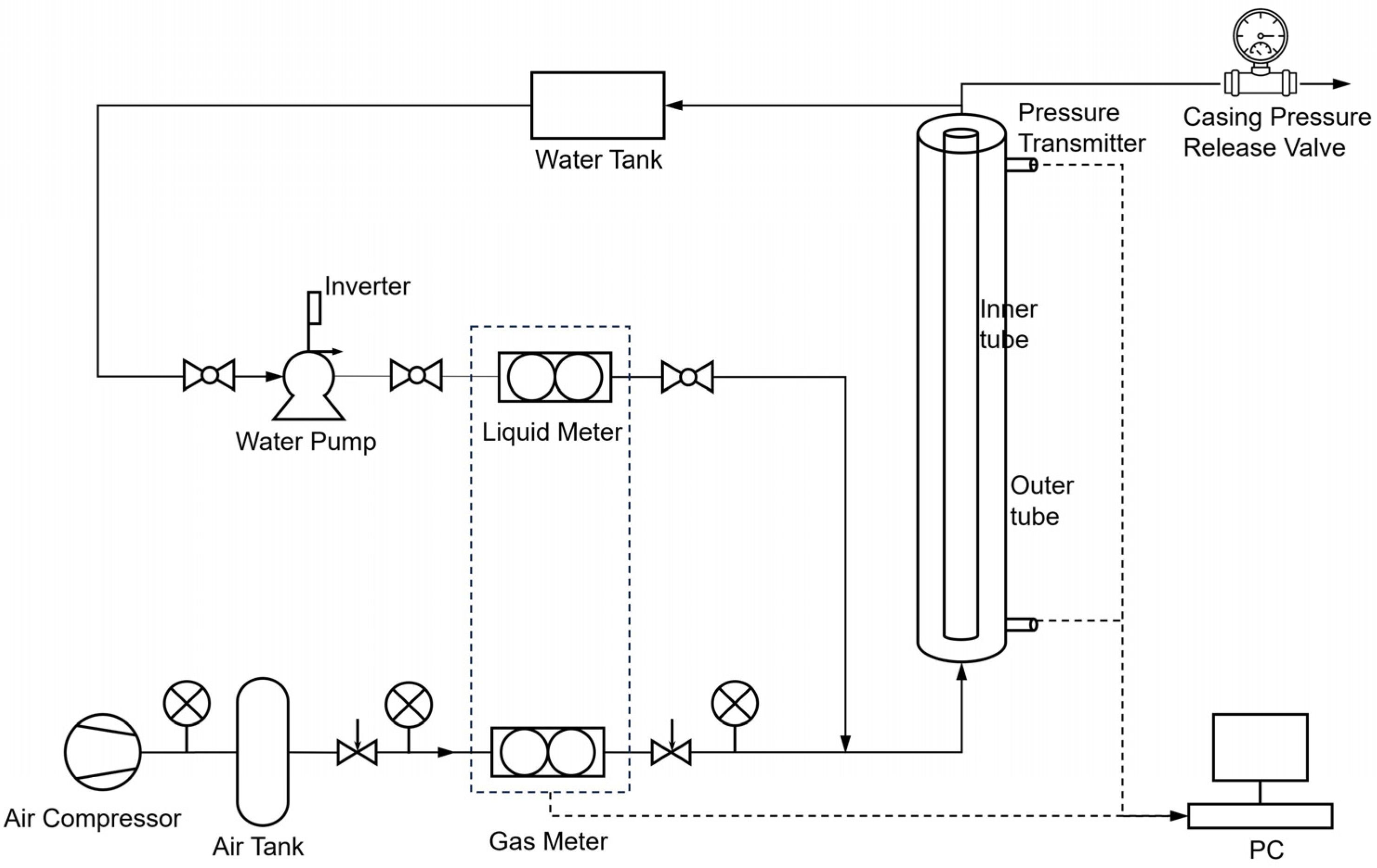
2.1. Experimental Apparatus

The experimental simulation device consists of four parts: gas injection system, water injection system, pipeline system, and monitoring system. Detailed experimental devices include water tank, water pump, liquid meter, air compressor, inverter, gas tank, gas meter, gas–liquid mixer, pressure transmitters, constant pressure release valve, plexiglass wellbore section, and measurement control system.

As a further improvement in this experiment, on the basis of conventional wellbore multiphase flow experimental equipment, a casing section is added outside the tubing section, and a constant pressure release valve (CPRV) is added at the casing head to control the casing pressure. During the experiment, when the gas inside the annulus continues to accumulate to the set pressure of the valve, the valve stem is pushed open by the gas pressure, allowing the casing gas to vent externally, resulting in a decrease in pressure. When the pressure drops to the set value, the valve stem is pushed down by the spring force, sealing the valve stem with the valve seat, and the gas no longer vents externally. As the gas reaccumulates and the pressure rises again, the valve stem is pushed open again to vent the gas. This process is repeated to achieve cyclic gas venting and control of the casing pressure. A gas–liquid mixer is installed at the bottom of the well to simulate reservoir production. To observe the fluctuation in the liquid level, the experimental tube section adopts the organic glass material with visual function and adds the water-based red dye to the water, simulating the annular multiphase flow through this device. The detailed experimental equipment and process are shown in Figure 1.

Liquid supply device: This device is used to supply a specified volume of water to the experimental device. The water is discharged from the water tank by the pump controlled by the frequency converter to form a water flow pipeline. The liquid flow rate is measured by the liquid flow meter, enters the gas–liquid mixer, and, finally, enters the experimental pipe section.

Gas supply device: This device is used to supply air at a specified flow rate to the experimental device. Compressed air is entered by the air compressor and stored in the air tank to form a gas pipeline. During the experiment, the valve at the back of the air tank is opened, the gas flow meter is used to monitor the air supplied by the air tank, and then it is entered into the gas–liquid mixer and, finally, into the experimental pipe section.

Visualization Wellbore device: This device is used to observe the gas–liquid flow pattern and liquid-level fluctuation in the annulus at different initial liquid-level heights and different gas flow rates. A graduated scale is attached to the outside of the outer pipe. When the gas flow rate stabilized, the liquid-level height H is read directly from the scale with an accuracy of 0.01 cm.

Experimental Measurement Devices: A gas flow meter is utilized to monitor the gas flow rate delivered from the air tank to the annulus, while a liquid flow meter is employed to monitor the water flow rate. Pressure transmitters are utilized to measure the upper pressure (wellhead) and lower pressure (bottomhole) in the outer pipe segment, with the casing pressure being controlled by the CPRV. Detailed information regarding the main measurement instruments used in the experiment is provided in the

Table 1. Detailed information table of experimental measuring instruments.

Experimental Measuring Instruments	Manufacturer	Type	Measurement Range	Accuracy
Gas Flow Meter	Beijing Qixing Huachuang Flowmeter Co., Ltd., Beijing, China	D07-60B	(0–1000) L/min	±2%
Liquid Flow Meter	ShanDong ShiYi Science and Technology Co., Ltd. of U.P.C, Dongying, China	LWGY-15(FL)/C3/05/W/S/E/N	(0.4–8) m3/h	±0.5%
Pressure Transmitter	Guangzhou Xisen Automation Control Equipment Co., Ltd., Guangzhou, China	BST6600-20BBIII1.0MPa0T0DNA938	(0–1.0) MPa	0.5 class
Constant Pressure Release Valve	Yancheng Haixuan Valve Co., Ltd., Yancheng, China	ZTP611-DKG-50	(0–0.6) MPa	±2%

.

2.2. Experimental Method and Procedure

Under ambient-temperature conditions, a total of 134 sets of ZNLF simulation experiments in the annulus were conducted at three casing pressures of 0.1 MPa, 0.3 MPa, and 0.5 MPa. The initial liquid column height in the annulus varied from 0.5 m to 2 m, and the gas injection rate ranged from 0.1 to 30 m³/h.

The pressures and gas injection rates chosen for experiments were designed to simulate the GLR at the suction inlet pressure of ESP wells. Through the similarity principle, the pump inlet pressure and gas flow rate of the actual ESP wells were converted into the pressure and gas flow rate under experimental conditions, so that the production conditions of the actual site could be simulated more realistically.

During the simulated experiments, the CPRV at the wellhead was initially closed, and water was injected into the bottom of the annulus until the water level reached the specified initial liquid column height. Subsequently, the water supply was stopped. A single-flow valve was installed at the inlet to prevent backflow. Gas was then injected into the bottom of the annulus at a predetermined rate. As the pressure in the annulus gradually increased due to the closure of the CPRV, the valve was opened when the pressure reached the specified casing pressure, stabilizing the pressure at the designated value. The flow patterns and fluctuations of the liquid level in the annulus were observed through transparent glass pipes.

Each experiment aimed to maintain ZNLF conditions, ensuring that no liquid was carried out of the wellhead by the gas, and a dynamic liquid level was maintained in the annulus, with gas production but no liquid production at the wellhead. The equivalent diameter of the annulus was determined by the difference between the casing inner diameter and the tubing outer diameter. The range of superficial gas velocity was calculated based on the gas injection rate and the cross-sectional area of the annulus, ranging from 0.007 to 2.3 m/s. Apart from injecting water to the specified initial height, no water entered the annulus during gas injection, and no water was produced at the wellhead, resulting in a stagnant liquid column in the annulus, thus yielding a superficial liquid velocity of 0 m/s in all experimental sets. Based on the conditions of ZNLF, the flow patterns, fluctuations in the dynamic liquid level, and changes in pressure drop in the annulus were investigated under different casing pressures, initial liquid column heights, and gas injection rates. The detailed experimental procedure is as follows:

(1)

Set up the annular experimental apparatus, check the air tightness of the apparatus, and connect the power supply.

(2)

Close the CPRV at the wellhead.

(3)

Start the air compressor to charge air into the air tank and then turn off the air compressor.

(4)

Open the liquid inlet valve and inject water into the annulus from the bottom of the pipe using a water pump until the water level reaches the specified initial height and then close the water pump.

(5)

Open the gas inlet valve and inject air into the annulus from the bottom of the pipe. Record the pressure of the CPRV in real time, i.e., the casing pressure. When the casing pressure reaches the specified value, open the CPRV to stabilize the casing pressure near the specified value. Observe the experimental phenomena in the annulus through the transparent pipe.

(6)

Capture corresponding photos and videos, record the flow patterns and the height of the dynamic liquid level in the annulus, and read the readings of the pressure transmitters at the wellhead and bottom of the well through the PC.

(7)

Repeat the experiment according to steps (2) to (6) by changing the casing pressure, initial liquid column height, and gas injection rate.

(8)

Process the obtained data to reveal the flow characteristics of ZNLF under different casing pressures, initial liquid column heights, and gas injection rates.

(9)

After the experiment, exhaust the water from the pipe, turn off the air compressor and water pump, and disconnect the experimental power supply.

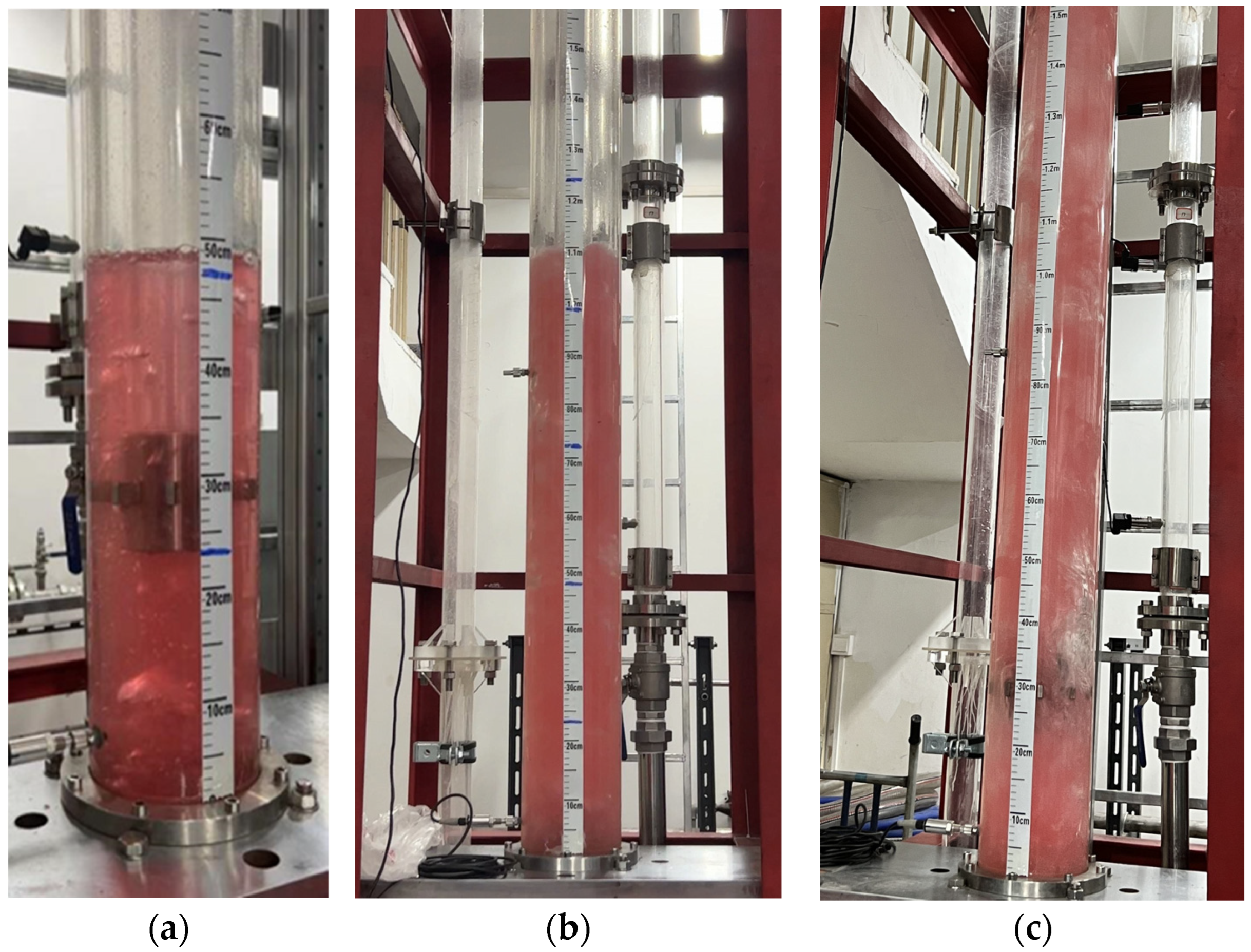
2.3. Experimental Phenomenon

The experimental results show that the air in the annulus is a dispersed phase, and the water is a continuous phase. The air enters the upper part of the annulus through the liquid column, and the slip-off between the air and the water is serious. From Figure 2, at low gas flow rates, the air is distributed in the liquid phase in the form of dispersed small bubbles, and the main flow pattern is bubble flow. At high gas flow rates, the air flows continuously through the liquid column to the upper part of the annulus and lifts the water. The gas velocity is relatively large, but it is not enough to keep the liquid droplets in suspension. The droplets fall and aggregate to form a liquid bridge. The main flow pattern is churn flow.

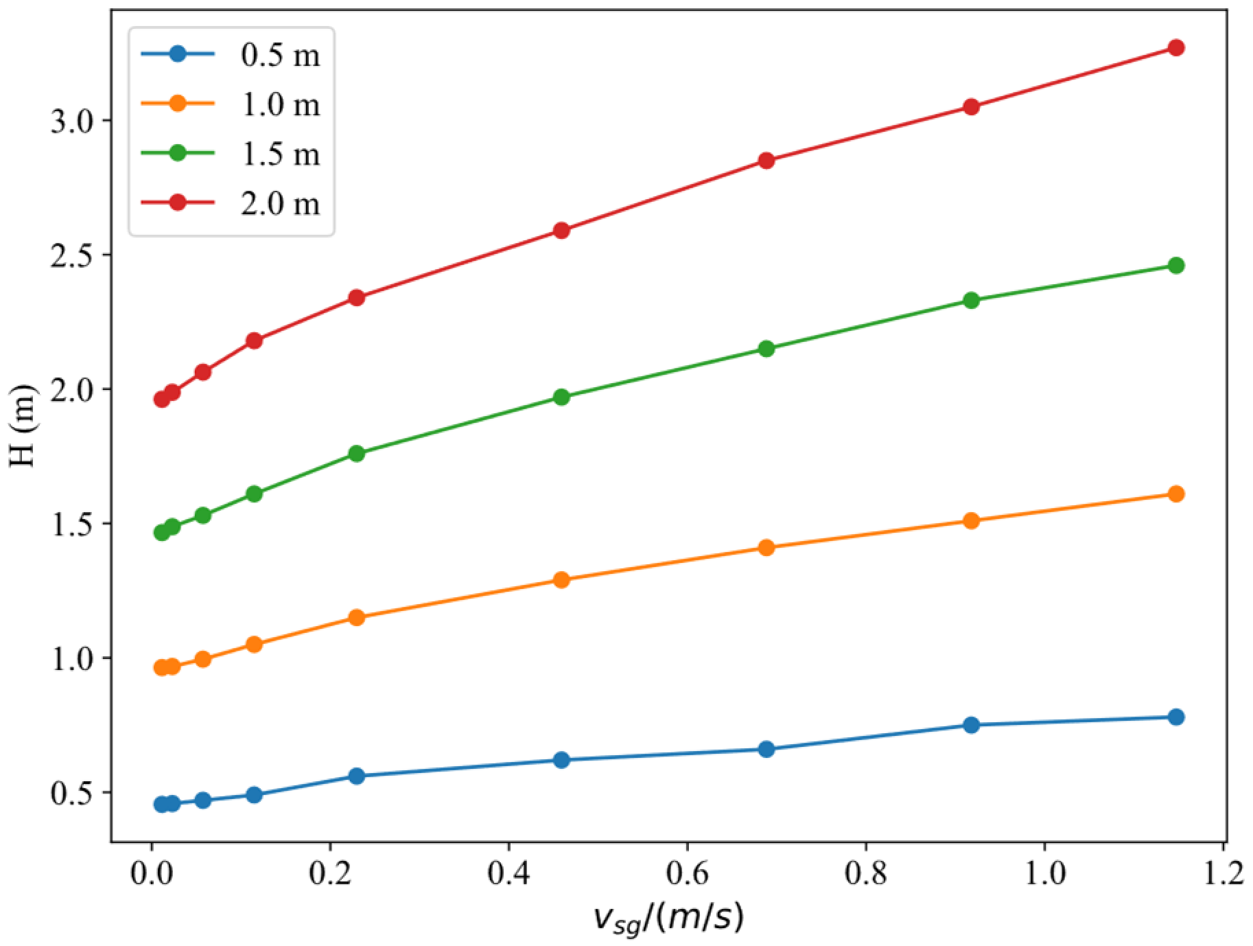
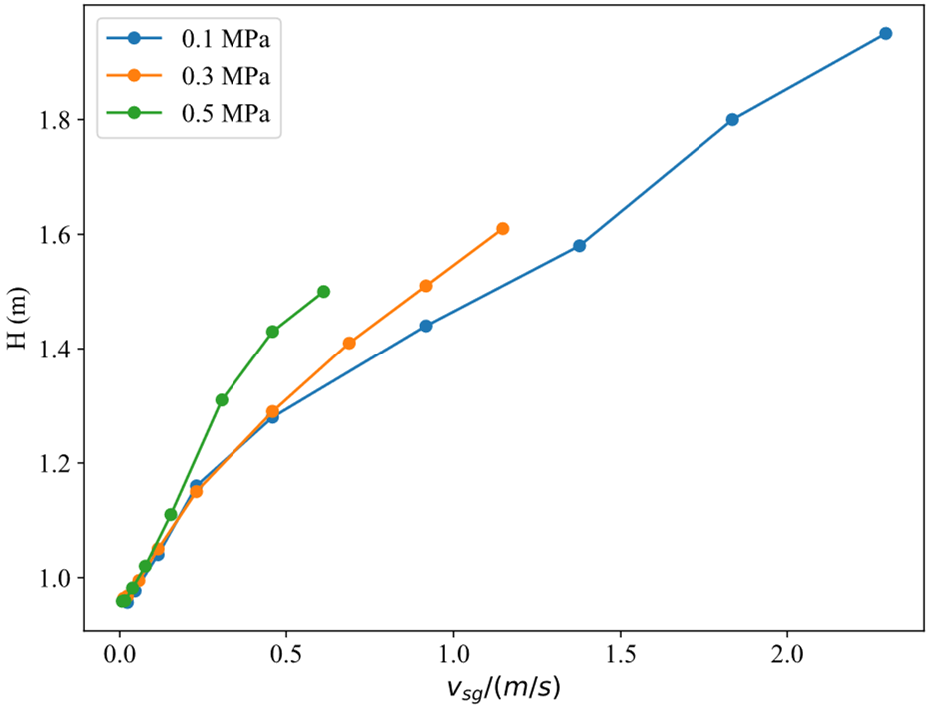
2.4. Experimental Results and Analysis

Potential sources of error in the experiments include:

(1)

Measurement Instrument Errors: Inaccuracies in the instruments used for measuring pressure, gas velocity, and liquid height can affect the precision of data.

(2)

Temperature Effects: Experiments did not account for temperature variations, which could influence fluid properties and flow dynamics.

(3)

Random Errors: Inherent variability in experimental conditions and measurements may introduce random errors.

Given the initial liquid-level height H₀, gas is injected into the annulus at a specified rate. Once the gas flow rate has stabilized, the new liquid-level height H is read. The expression for the annular average holdup is as follows:

$$HO{L}_{ave}=\frac{H_0}{H}$$

(1)

where H₀ is the initial liquid-level height, IN m; H is dynamic liquid-level height, IN m; HOL_ave is the annular average holdup, dimensionless.

Pressure transmitters are used to measure the pressure at the top and bottom of the outer pipe. The pressure drop of the annulus is determined by subtracting the wellhead pressure from the bottomhole pressure.

$$\mathrm{\Delta }P=P_{BH}-P_{WH}$$

(2)

$$\frac{dP}{dh}=\frac{\mathrm{\Delta }P}{H}$$

(3)

where P_BH is the bottomhole pressure, IN Pa; P_WH is the wellhead pressure, IN Pa; ΔP is the pressure drop, IN Pa.

The equivalent diameter of the annulus is calculated as the inner diameter of the casing minus the outer diameter of the tubing [23],the following formula:

$$d_e=d_c-d_t$$

(4)

where d_t is the outer diameter of the tubing, IN m; d_c is the inner diameter of the casing, IN m. d_e is the equivalent diameter of the annulus, IN m.

The superficial gas velocity is determined by dividing the gas injection rate by the cross-sectional area of the annulus.

$$v_{sg}=\frac{Q_g}{A}$$

(5)

where v_sg is the superficial gas velocity, IN m/s; Q_g is the gas injection rate, IN m³/s; A is the cross-sectional area of the annulus, IN m².

The experimental results indicated that the predominant flow patterns in the annular ZNLF were bubble flow and churn flow. Bubble flow was observed at lower gas flow rates, while churn flow was observed at higher gas flow rates.

The variation trend of the dynamic liquid level in the annulus with v_sg is depicted in Figure 3 and Figure 4. Figure 3 illustrates the change in dynamic liquid level with v_sg at a casing pressure of 0.3 MPa for different initial liquid column heights.

From Figure 3, it can be observed that when the casing pressure and initial liquid column height are the same, the height of the liquid column in the annulus increases with the increase in v_sg. This is because, with the casing pressure maintained constant and gas injected into the well bottom, the gas starts accumulating at the bottom of the annulus, forming a pressure zone [24]. As more gas is injected, v_sg gradually increases, and the volume of this pressure zone increases. To maintain pressure balance within the annulus, the gas pushes the liquid above it upward. Therefore, with an increasing v_sg, the height of the liquid column gradually rises. Additionally, it can be noted that, at the same velocity, the higher the initial liquid column, the higher the dynamic liquid level.

Figure 4 shows the change in liquid column height with v_sg under different casing pressures, with an initial liquid column height of 1 m. It is evident that under the same gas velocity, higher casing pressure results in a higher dynamic liquid level. Increased casing pressure compresses the gas inside the annulus, causing the liquid level to rise to maintain balance between gas and liquid pressures [25,26].

Figure 5 represents the holdup variation with v_sg for different initial liquid column heights at a casing pressure of 0.3 MPa. It can be observed that, under the same casing pressure and initial liquid column height, the holdup decreases as v_sg increases. Additionally, at the same gas velocity, the variation in holdup is not significant for different initial liquid column heights. This indicates that, under the same casing pressure, the holdup is not significantly affected by the amount of liquid inside the annulus.

Figure 6 depicts the variation in holdup with v_sg for different casing pressures when the initial liquid column height is 1 m. It can be observed that under the same gas velocity, a higher wellhead casing pressure leads to a lower holdup. This indicates that higher casing pressure compresses the gas inside the annulus, causing the liquid level to rise, thus resulting in a reduction in the cross-sectional holdup [27].

The total pressure drop is composed of gravity pressure drop, friction pressure drop, and kinetic energy pressure drop. The proportion of pressure drop caused by the kinetic energy term is small and negligible. Holdup is determined based on the dynamic liquid level, allowing for the calculation of gravitational pressure drop. Therefore, the frictional pressure drop can be obtained by the difference between the total pressure drop and the gravitational pressure drop.

Figure 7 depicts the variations in the total pressure drop gradient, gravitational pressure drop gradient, and frictional pressure drop gradient with v_sg under a wellhead casing pressure of 0.3 MPa. It can be observed that both the total pressure gradient and the gravitational pressure gradient decrease with increasing v_sg, while the frictional pressure gradient increases with increasing v_sg. This trend arises because as the gas volume increases, v_sg also increases, leading to a reduction in the holdup inside the annulus, consequently resulting in a decrease in both the gravitational pressure gradient and the total pressure gradient inside the pipe. Moreover, the higher gas velocity intensifies the dynamic complexity of the fluid, including changes in flow patterns and increased disturbance of the gas–liquid interface, thereby enhancing friction between the gas–liquid phase and the pipe wall and causing an increase in the frictional pressure gradient.

Next, we focus solely on the analysis of the frictional pressure gradient.

Table 2. Frictional pressure gradient with v_sg at 0.3 MPa.

vsg (m/s)	0.011	0.023	0.057	0.115	0.229	0.459	0.688	0.918	1.147
dPf/dh (KPa/m) (0.5 m)	−0.483	−0.425	0.088	0.974	1.164	1.999	1.958	2.143	2.373
dPf/dh (KPa/m) (1.0 m)	−0.371	−0.113	−0.108	0.075	0.184	0.740	0.809	0.977	1.033
dPf/dh (KPa/m) (1.5 m)	−0.269	−0.085	−0.159	0.207	0.202	0.483	0.548	0.620	0.647
dPf/dh (KPa/m) (2.0 m)	−0.393	−0.369	−0.219	0.003	0.105	0.298	0.311	0.422	0.430

shows the change in the friction pressure gradient with v_sg corresponding to the initial liquid column heights of 0.5 m, 1 m, 1.5 m, and 2 m when the casing pressure is 0.3 MPa.

When v_sg is low (less than 0.057 m/s), the frictional pressure gradient is negative for all experiments. This is because, when the gas flow rate is low, gas bubbles pass through the stationary liquid column towards the gas section above the annulus. During this process, the liquid film around the bubbles flows downward, and the frictional force acting on the liquid film is directed upward. When the frictional force acting on the liquid film exceeds the frictional force causing the bubbles to move upward, the frictional pressure gradient becomes negative [19,28]. This phenomenon also demonstrates the uniqueness of ZNLF. Then, we converted the data into the form of a picture, as shown in Figure 8.

Figure 8 depicts the relationship between the frictional pressure gradient and v_sg under different initial liquid-level heights when the casing pressure is 0.3 MPa. It can be observed that the frictional pressure gradient increases with increasing v_sg. In addition, it can be found that the frictional pressure gradient decreases with the increase in the height of the liquid column at the same v_sg. This is because when the height of the liquid level is lower, the resistance that the gas can overcome to pass through the liquid column is smaller, which makes the friction between the gas–liquid mixed flow and the pipe greater.

3. Theoretical Model of ZNLF in Annulus

The model of ZNLF in annulus is different from that of conventional gas–liquid two-phase flow. When the ESP well is in production, the liquid phase stays in the annulus during the casing gas-venting process, the bubble passes through the liquid section into the special state of the gas column above the annulus, and the holdup is more serious. Therefore, the conventional two-phase flow model cannot be used directly to calculate the ZNLF in the annulus.

3.1. Pressure Drop Gradient

It can be seen from the experimental results that the main flow modes of ZNLF are bubble flow and churn flow. Therefore, we established a pressure drop calculation model suitable for bubble flow and churn flow under the annular ZNLF.

The mass conservation equation of mixed fluid is as follows [21]:

$$\frac{\partial }{\partial h}({\rho }_m{v}_m)+\frac{\partial {\rho }_m}{\partial t}=0$$

(6)

where ρ_m is the density of the gas–liquid mixture, IN kg/m³; v_m is the velocity of the gas–liquid mixture, IN m/s; h is the depth of the wellbore, IN m; t is time, IN s.

The momentum conservation equation [21] of the mixed fluid is:

$$\frac{\partial }{\partial t}({\rho }_m{v}_m)+\frac{\partial P}{\partial h}+{\rho }_{m}g+\frac{2f{\rho }_m{v}_m^2}{d_e}=0$$

(7)

where f is coefficient of friction, dimensionless; P is pressure, IN Pa. After simplifying the momentum equation, the formula for calculating pressure drop is obtained:

$$\frac{dP}{dh}=-{\rho }_{m}g-\frac{2f{\rho }_m{v}_m^2}{d_e}-{\rho }_m{v}_m\frac{d{v}_m}{dh}$$

(8)

In the calculation of annular multiphase flow pressure drop, it is very important to estimate the holdup, which directly determines the physical properties of the mixed fluid.

3.1.1. Bubble Flow

The velocity of the gas phase is equal to the superficial velocity of the gas phase divided by the void fraction. For the bubble flow with ZNLF in the annulus, the void fraction is expressed by the following formula [23]:

$$f_g=\frac{v_{sg}}{C_0{v}_m+v_{\infty }}=\frac{v_{sg}}{C_0(v_{sg}+v_{sl})+v_{\infty }}$$

(9)

where f_g is the void fraction, dimensionless; C₀ is the flow coefficient, representing the change in velocity and bubble concentration of the two-phase mixture, dimensionless; v_∞ is the terminal velocity of Taylor bubbles rising, IN m/s; v_sl is the superficial liquid velocity, IN m/s.

Since the superficial velocity of the liquid phase of the stagnant liquid column is 0, the following formula can be obtained after simplification:

$$f_g=\frac{v_{sg}}{C_0{v}_{sg}+v_{\infty }}$$

(10)

Hasan and Kabir believed that C₀ is related to the pipe diameter ratio [23] and obtained the relationship between C₀ and the pipe diameter ratio:

$$C_0=1.97+0.371\frac{d_t}{d_c}$$

(11)

For v_∞, use the Harmathy relation [29]:

$$v_{\infty }=1.53{\left[g\sigma ({\rho }_l-{\rho }_g)/{\rho }_l^2\right]}^{0.25}$$

(12)

where σ is the surface tension, IN N/m; ρ_l is the liquid density, IN kg/m³; ρ_g is the gas density, IN kg/m³; g is the acceleration of gravity, IN m/s².

Therefore, the expression of the void fraction under the bubble flow pattern is obtained [23]:

$$f_g=\frac{v_{sg}}{(1.97+0.371\frac{d_t}{d_c})v_{sg}+1.53{\left[g\sigma ({\rho }_l-{\rho }_g)/{\rho }_l^2\right]}^{0.25}}$$

(13)

Equation (13) is used to predict the void fraction of the bubble flow and calculate the physical properties of the gas–liquid mixed fluid, which is brought into Equation (8).

Relevant studies have shown that the presence of inner tubes can affect the development of gas bubbles [30]. For the calculation of frictional pressure drop under the bubble flow pattern, Newton’s classical mechanics theory was used to analyze the force of the bubble. As shown in Figure 9, the bubble is subjected to upward buoyancy force, downward gravity, and friction force. The direction of vertical upward flow of bubbles is defined as positive, according to Newton’s second law [31]:

$$F_f+G+F_d=m\frac{\mathrm{d}{v}_{\mathrm{d}}}{\mathrm{d}t}$$

(14)

where F_f is the buoyancy force of the bubble, IN N; G is the bubble gravity, IN N; F_d is the resistance of the bubble flow process, IN N; m is the bubble mass, IN kg; v_d is the floating velocity of the bubble, IN m/s; t is the floating time of the bubble, IN s. Assuming that the bubble flow process is uniformly rising, Equation (14) can be written as:

$$\frac{1}{6}\pi {\rho }_{1}g{d}^3-\frac{1}{6}\pi {\rho }_{\mathrm{g}}g{d}^3-\frac{1}{8}\pi {\rho }_1{C}_{\mathrm{d}}{v_{\mathrm{d}}}^2{d}^2=0$$

(15)

where C_d is the resistance coefficient, dimensionless, which is 1.48; d is the bubble diameter, IN m. After simplifying Equation (15), the bubble floating velocity is as follows [31]:

$$v_d^2=\frac{4\left({\rho }_{\mathrm{l}}-{\rho }_{\mathrm{g}}\right)gd}{3{\rho }_{\mathrm{l}}{C}_{\mathrm{d}}}$$

(16)

Since small bubbles obey Stokes theorem, when the diameter of the bubble is less than 0.05 cm [32], the local slip velocity of the small bubble is:

$$V_{2j}=\frac{g\left({\rho }_{\mathrm{l}}-{\rho }_{\mathrm{g}}\right)d^2}{18{\mu }_1}{(1-f_g)}^3$$

(17)

where V_2j is the local slip velocity of the small bubble, IN m/s; μ_l is the viscosity of the liquid phase, IN Pa.s.

When the diameter of the bubble is 0.1 cm~2 cm, the local slip velocity of the bubble is [32]:

$$V_{2j}=1.53{\left[\frac{\sigma g\left({\rho }_{\mathrm{l}}-{\rho }_{\mathrm{g}}\right)}{{{\rho }_1}^2}\right]}^{1/4}{(1-f_g)}^{3/2}$$

(18)

The rising speed of the bubble is:

$$v_g=v_{sg}+v_{2j}$$

(19)

where v_g is the real velocity of the bubble, IN m/s.

The diameter of the bubble is calculated by combining Equations (16)–(18) or Equations (16), (17), and (19); the buoyancy force of the bubble is equal to the aggravating force of friction, and the friction force can be calculated.

By adding the three components of the pressure drop model, the total pressure drop gradient in the well annulus flow can be obtained.

3.1.2. Churn Flow

The churn flow is regarded as the combination of slug flow and bubble flow in a special state, and the liquid film zone and the liquid slug zone are considered as one system. As shown in the figure below, L_f represents the liquid film zone and L_s represents the liquid slug zone.

The churn flow is simplified by the physical model shown in Figure 10, and the compressibility of the fluid is ignored to establish a mathematical model of ZNLF in the annulus. The average holdup can be expressed as [18]:

$$H_L=\frac{H_f{L}_f+H_s{L}_s}{L_f+L_s}$$

(20)

where H_f is the holdup in the liquid film region, dimensionless; H_s is the holdup in the liquid slug region, dimensionless; L_f is the length of liquid film region, IN m; L_s is the length of the liquid slug zone, IN m; H_L is the average holdup, dimensionless.

The average liquid phase velocity is [18]:

$$v_l=\frac{Q_l}{H_{L}A}=\frac{v_s{H}_s{L}_s+v_{lf}{H}_f{L}_f}{L_f+L_s}$$

(21)

where v_l is the average liquid-phase velocity, IN m/s; v_s is the average velocity of the liquid slug zone, IN m/s; v_lf is the liquid-phase velocity of liquid film region, IN m/s; Q_l is the liquid-phase flow rate, IN m³/s.

Since there is ZNLF, so v_l = 0, Equation (21) is simplified as:

$$v_s{H}_s{L}_s+v_{lf}{H}_f{L}_f=0$$

(22)

Taking the liquid phase as the research object, the equilibrium equation of liquid phase in the liquid film region and liquid slug region is as follows [18,19]:

$$H_f(v_t-v_{lf})=H_s(v_t-v_s)$$

(23)

where v_t is the rising velocity of Taylor bubbles, IN m/s; v_s is approximately equal to the mixing velocity v_m of the gas–liquid two phases. For ZNLF, v_m is equal to the gas phase superficial gas velocity v_sg:

$$v_s=v_m=\frac{Q_g}{A}=v_{sg}$$

(24)

Equations (20), (22)–(24) are simplified to obtain the calculation formula of holdup:

$$H_L=H_s(1-\frac{v_{sg}}{v_t})$$

(25)

where H_s can be calculated from Gregory’s relation [33]:

$$H_s=\frac{1}{1+{(v_m/8.66)}^{1.39}}$$

(26)

v_t is commonly used in multiphase flows as follows:

$$v_t=C_0{v}_m+v_{\infty }$$

(27)

Express Equation (10) in the form of Equation (28):

$$\frac{v_{sg}{H}_s}{H_s-H_l}=C_0{v}_{sg}+v_{\infty }$$

(28)

The experimental data were analyzed, and the curve was drawn with v_sgH_s/(H_s − H_l) as the ordinate and v_sg as the abscissa. It can be seen from the plot that the curve is approximately a linear function, where the slope represents the flow coefficient C₀ and the intercept represents the slip velocity v_∞. It can be seen from the results that the intercept of each group of experimental curves is different, which means that the casing pressure affects the slip velocity v_∞.

To estimate the holdup under churn flow, a modified form of Equation (28) is proposed:

$$\frac{H_s-H_l}{H_s}=\frac{v_{sg}}{C_0{v}_{sg}+k_c\sqrt{g{d}_e({\rho }_l-{\rho }_g)/{\rho }_l}}$$

(29)

According to the experimental results, C₀ is 1.97, and k_c represents the coefficient of slip velocity v_∞, dimensionless, which is related to casing pressure P_c. According to the experimental results, k_c has the following relationship with P_c:

$$k_c=1.94455e^{-2{.131\mathrm{P}}_c\times {1\mathrm{e}}^{-6}}$$

(30)

where P_c is the casing pressure, IN Pa;

Therefore, the formula for calculating holdup under churn flow is obtained:

$$\frac{H_s-H_l}{H_s}=\frac{v_{sg}}{1.97v_{sg}+(1.94455e^{-2{.131\mathrm{P}}_c\times {1\mathrm{e}}^{-6}})\sqrt{g{d}_e({\rho }_l-{\rho }_g)/{\rho }_l}}$$

(31)

For the frictional pressure drop, because the liquid is at rest and Reynolds number is invalid, the method of calculating frictional pressure drop with conventional two-phase flow cannot be used to calculate the frictional pressure drop with ZNLF. The frictional pressure drop with ZNLF can be expressed as [18,34]:

$$\mathrm{\Delta }{P}_{\mathrm{F}}=\frac{L_{\mathrm{p}}}{L_{\mathrm{s}}+L_{\mathrm{f}}}(\frac{{\tau }_{\mathrm{s}}\pi d_e{L}_{\mathrm{s}}}{A}+\frac{{\tau }_{\mathrm{lf}}\pi d_e{L}_{\mathrm{f}}}{A})$$

(32)

where τ_s is the shear stress between the liquid slug and the wall, IN Pa; τ_lf is the shear stress between the liquid film and the wall, IN Pa; L_p is pipe length, IN m; ΔP_F is the friction pressure drop, IN Pa.

Taking the liquid film region as the research object, the momentum conservation equations are established for the flow of the liquid film and the Taylor bubble [34], as shown in Equations (33) and (34), respectively.

$$A_l{\left(-\frac{dP}{dh}\right)}_l={\rho }_{1}g{A}_l-{\tau }_{lf}{S}_{lf}+{\tau }_{\mathrm{i}}{S}_{\mathrm{i}}$$

(33)

$$A_g{\left(-\frac{dP}{dh}\right)}_g={\rho }_{g}g{A}_g+{\tau }_{gf}{S}_{gf}-{\tau }_{\mathrm{i}}{S}_{\mathrm{i}}$$

(34)

where τ_gf is the shear stress between the Taylor bubble and the wall, IN Pa; τ_i is the shear stress at the gas–liquid two-phase interface, IN Pa; A_l is the area of the liquid phase flow channel, IN m²; A_g is the area of the gas-phase flow channel, IN m²; S_lf is the wet circumference of liquid phase, IN m; S_gf is the wet circumference of gas phase, IN m; S_i is the wet circumference of the gas–liquid two-phase contact surface, IN m.

Under steady-state conditions, it can be considered that:

$${\left(-\frac{dP}{dh}\right)}_l={\left(-\frac{dP}{dh}\right)}_g$$

(35)

Equations (33)–(35) yield [18]:

$$\frac{{\tau }_f\pi D}{H_{\mathrm{f}}}+{\tau }_{\mathrm{i}}{S}_{\mathrm{i}}\left(\frac{1}{H_{\mathrm{f}}}+\frac{1}{1-H_{\mathrm{f}}}\right)-({\rho }_1-{\rho }_{\mathrm{g}})gA=0$$

(36)

The mass conservation of liquid flow in the liquid film region is Equation (23), and the mass conservation equation is established for Taylor bubbles in the liquid film region, as follows [19]:

$$(1-H_f)(v_t-v_{gf})=H_s(v_t-v_s)$$

(37)

where v_gf is the liquid-phase flow rate in the liquid film region, IN m/s. τ_lf is a function of v_lf, τ_lf is a function of v_lf and v_gf. By connecting Equations (23), (36), and (37), we can obtain the v_lf, v_gf and H_f. For the superficial gas velocity, there is the following expression [19]:

$$v_{sg}=\frac{L_f}{L_f+L_s}(1-H_f)v_{gf}+\frac{L_s}{L_f+L_s}(1-H_s)v_m$$

(38)

By connecting Equations (22) and (38), we can obtain the L_s and L_f. The friction pressure drop can be calculated by bringing it into Equation (32).

The total pressure drop of ZNLF is the sum of gravitational pressure drop and frictional pressure drop. Therefore, the total pressure drop [18,21,34] of the churn flow is:

$$\mathrm{\Delta }P=\mathrm{\Delta }{P}_{\mathrm{F}}+\left[\begin{array}{c}{H}_1{\rho }_1+(1-H_1){\rho }_g\end{array}\right]g{\mathrm{L}}_{\mathrm{p}}$$

(39)

3.2. Flow Pattern Transitions

The holdup conversion condition of bubble flow is 0.75 [23,35], so the distinguishing condition of the bubble flow pattern is:

$$v_{sg}\le 0.4829\sqrt[4]{\frac{g\sigma ({\rho }_l-{\rho }_g)}{{\rho }_l^2}}$$

(40)

The criterion of churn flow pattern is [21]:

$$0.4829\sqrt[4]{\frac{g\sigma ({\rho }_l-{\rho }_g)}{{\rho }_l^2}}<v_{sg}\le 3.1\sqrt[4]{\frac{g\sigma ({\rho }_l-{\rho }_g)}{{\rho }_g^2}}$$

(41)

The two-phase flow model established is suitable for calculating the pressure drop and holdup in the annulus for bubbly flow and churn flow, where the gas flow rate is not excessively high. As observed in Equation (41), if the superficial gas velocity exceeds its upper limit, there is a risk of the gas flow rate becoming too large, potentially carrying the liquid out of the wellhead. In such cases, the model would no longer be applicable.

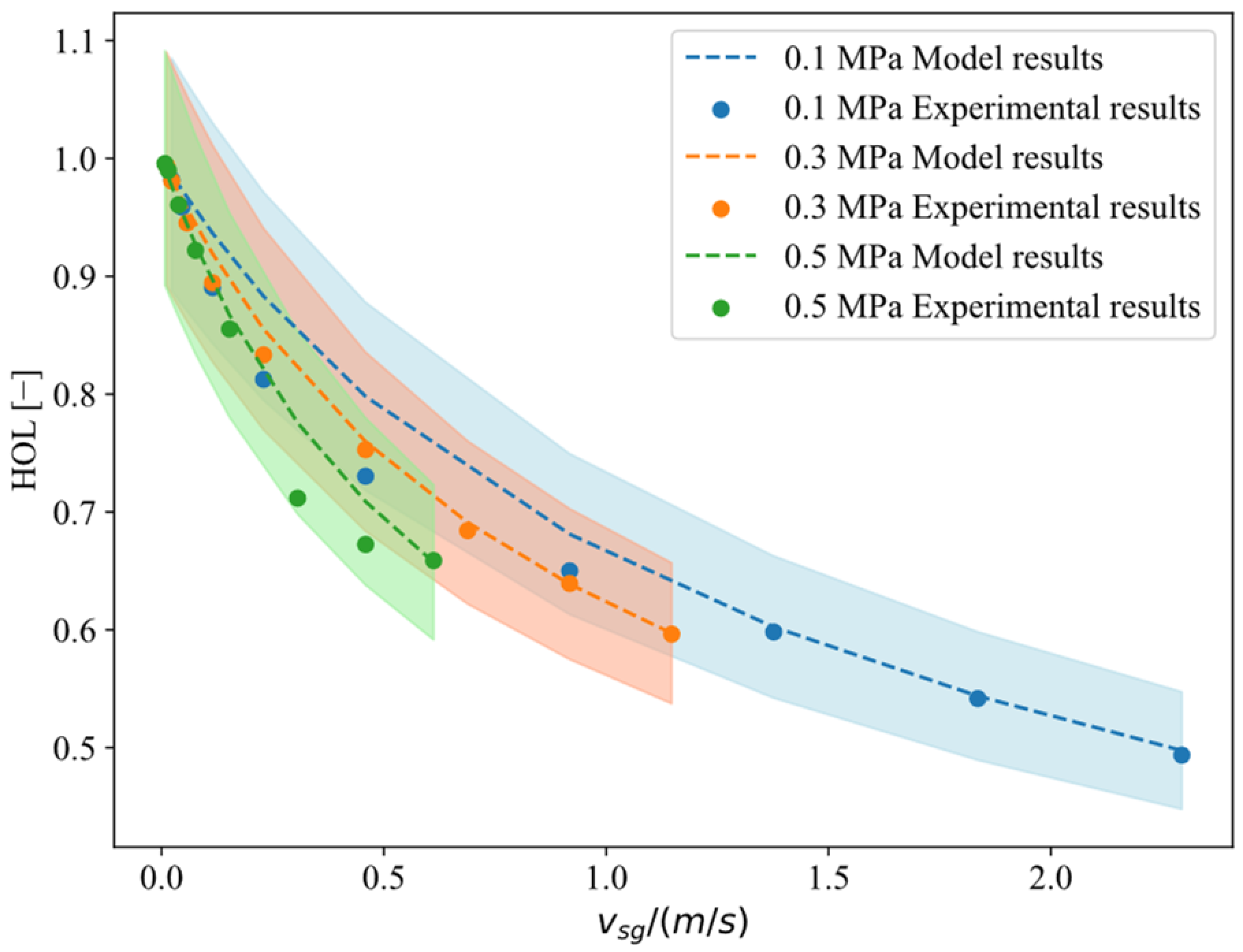
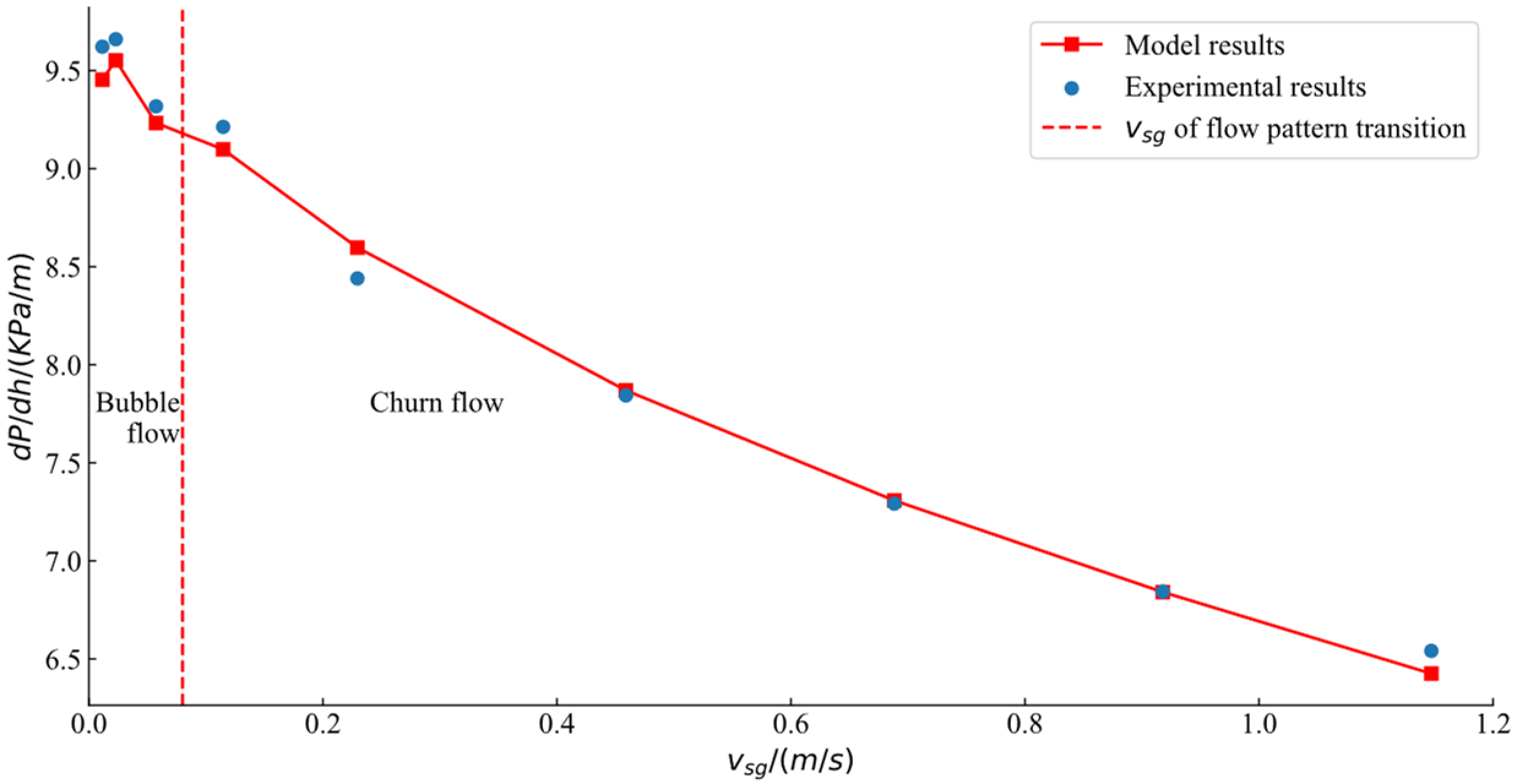
4. Model Verification

The accurate estimation of holdup is crucial for predicting the pressure along the annulus. In order to verify the established model of HOL, experimental data were used to test the ZNLF model, and the comparison results are shown in

Table 3. Comparative results of holdup.

vsg (m/s)	0.011	0.023	0.057	0.115	0.229	0.459	0.688	0.918	1.147
HOL (Experiment)	0.994	0.981	0.945	0.894	0.833	0.753	0.684	0.639	0.596
HOL (Model)	0.991	0.982	0.957	0.919	0.855	0.760	0.691	0.639	0.597
errHOL (%)	−0.286	0.141	1.266	2.765	2.614	0.890	1.004	−0.083	0.127

. The formula for calculating the relative deviation of liquid holdup is shown in Equation (42):

$$er{r}_{HOL}=\frac{HO{L}_{ZNLF}-HO{L}_{Exp}}{HO{L}_{Exp}}$$

(42)

where err_HOL is the relative deviation in liquid holdup, IN %;

It can be seen that the holdup predicted by the model is not much different from the experimental results, and the maximum error is 2.765%.

Using the ZNLF model, the holdup under different casing pressures was calculated with an initial liquid column height of 2 m, as shown in Figure 11. As shown in the figure, all three sets of calculated results are within a 10% error margin, indicating that the established model has high accuracy. Additionally, at the same v_sg, the higher the casing pressure, the lower the liquid holdup. The magnitude of the casing pressure affects the fluctuation in the dynamic liquid level. When the casing pressure at the wellhead increases, the dynamic liquid level in the annulus rises. This is mainly because the increased external casing pressure compresses the internal gas more, thus requiring a higher liquid column to balance this pressure difference.

Ignoring the kinetic energy term, the total pressure drop gradient is composed of the gravity pressure drop gradient and frictional pressure drop gradient. The ZNLF model is used to calculate the pressure drop gradient, and the results were compared with the experimental pressure drop results, as shown in

Table 4. Comparative results of pressure drop gradient.

vsg (m/s)	0.011	0.023	0.057	0.115	0.229	0.459	0.688	0.918	1.147
dP/dh (KPa/m) (Experiment)	9.622	9.660	9.318	9.213	8.440	7.844	7.292	6.843	6.541
dP/dh (KPa/m) (Model)	9.454	9.552	9.233	9.098	8.598	7.869	7.308	6.841	6.425
errΔp (%)	−1.749	−1.115	−0.912	−1.245	1.865	0.329	0.218	−0.038	−1.773

.

$$er{r}_{\mathrm{\Delta }P}=\frac{{\left(\frac{dP}{dh}\right)}_{ZNLF}-{\left(\frac{dP}{dh}\right)}_{Exp}}{{\left(\frac{dP}{dh}\right)}_{Exp}}$$

(43)

where err_Δp is the relative deviation of the pressure drop gradient, IN %;

Using the ZNLF model, the pressure gradient is calculated under a casing pressure of 0.3 MPa and an initial liquid column height of 2 m, with varying v_sg. A comparison of the model results with the experimental results is shown in Figure 12.

Compared to churn flow, the holdup in bubble flow decreases more rapidly with increasing v_sg. The flow pattern transition occurs at a superficial gas velocity of approximately 0.08 m/s, changing from bubble flow to churn flow. In addition, bubble flow has a higher holdup, resulting in a greater gravity pressure drop. This makes the total pressure drop gradient in bubble flow greater than that in churn flow.

5. Conclusions

To study the flow characteristics of casing pressure-controlled gas-venting wells, this study proposes an experimental simulation method for ZNLF in the annulus of a casing. By controlling the casing pressure, initial liquid column height, and gas injection rate, the ZNLF flow in the annulus is maintained. Additionally, a mathematical model for ZNLF in the annulus, considering liquid holdup, is established. The following conclusions were drawn from this study:

(1)

The experimental results show that the main flow patterns of ZNLF in the annulus are bubble flow and churn flow. At low gas flow rates, bubble flow dominates, while at high gas flow rates, churn flow prevails. Additionally, due to liquid-phase retention in the annulus, slip loss and holdup are more pronounced.

(2)

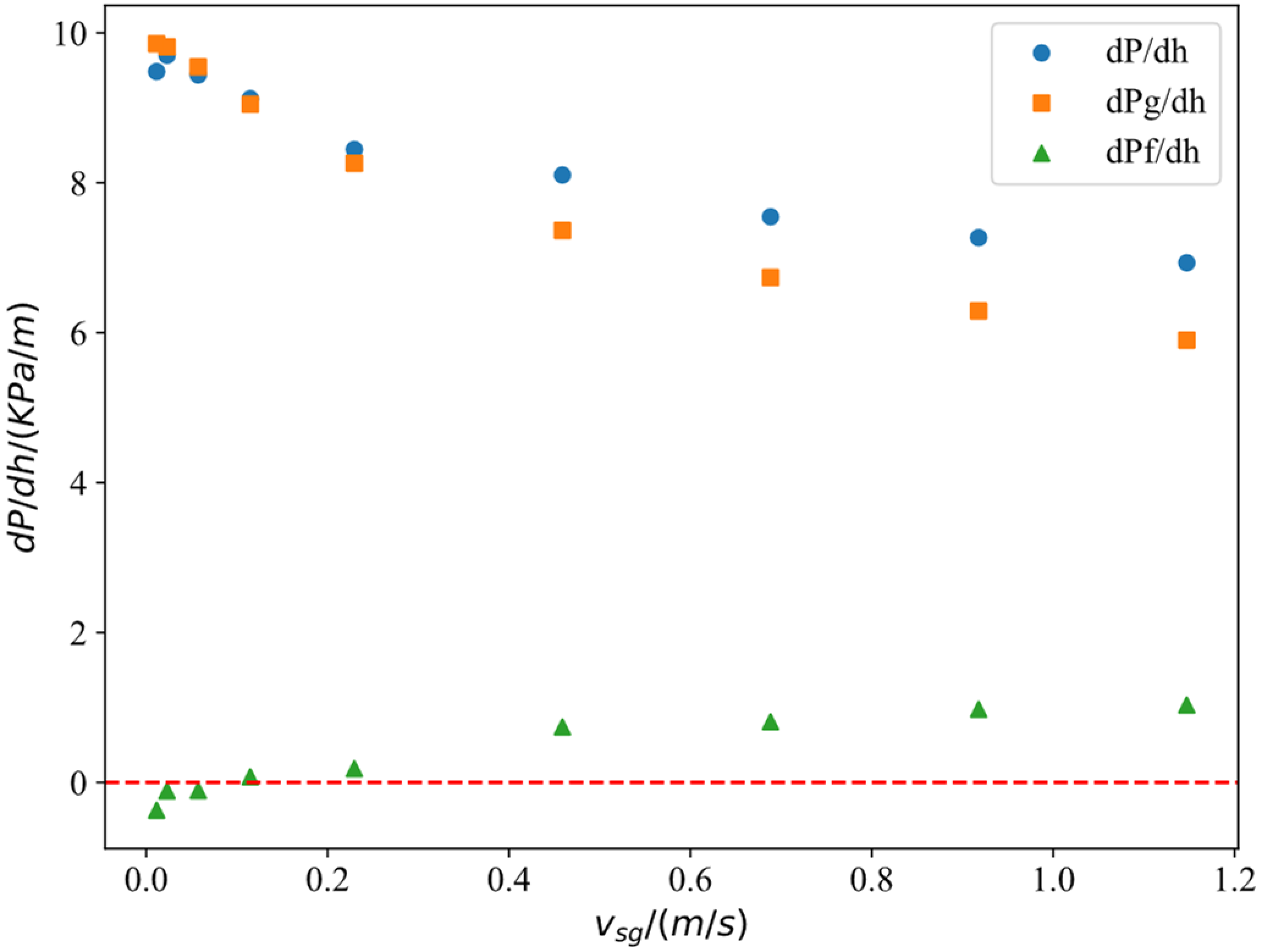
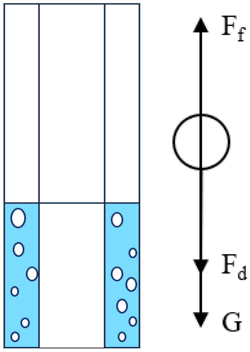
The experiments indicate that at low gas flow rates, the frictional pressure drop is negative. This is because the frictional force exerted by the downward-moving liquid film in contact with the rising bubbles is greater than the frictional force exerted on the upward-moving bubbles.

(3)

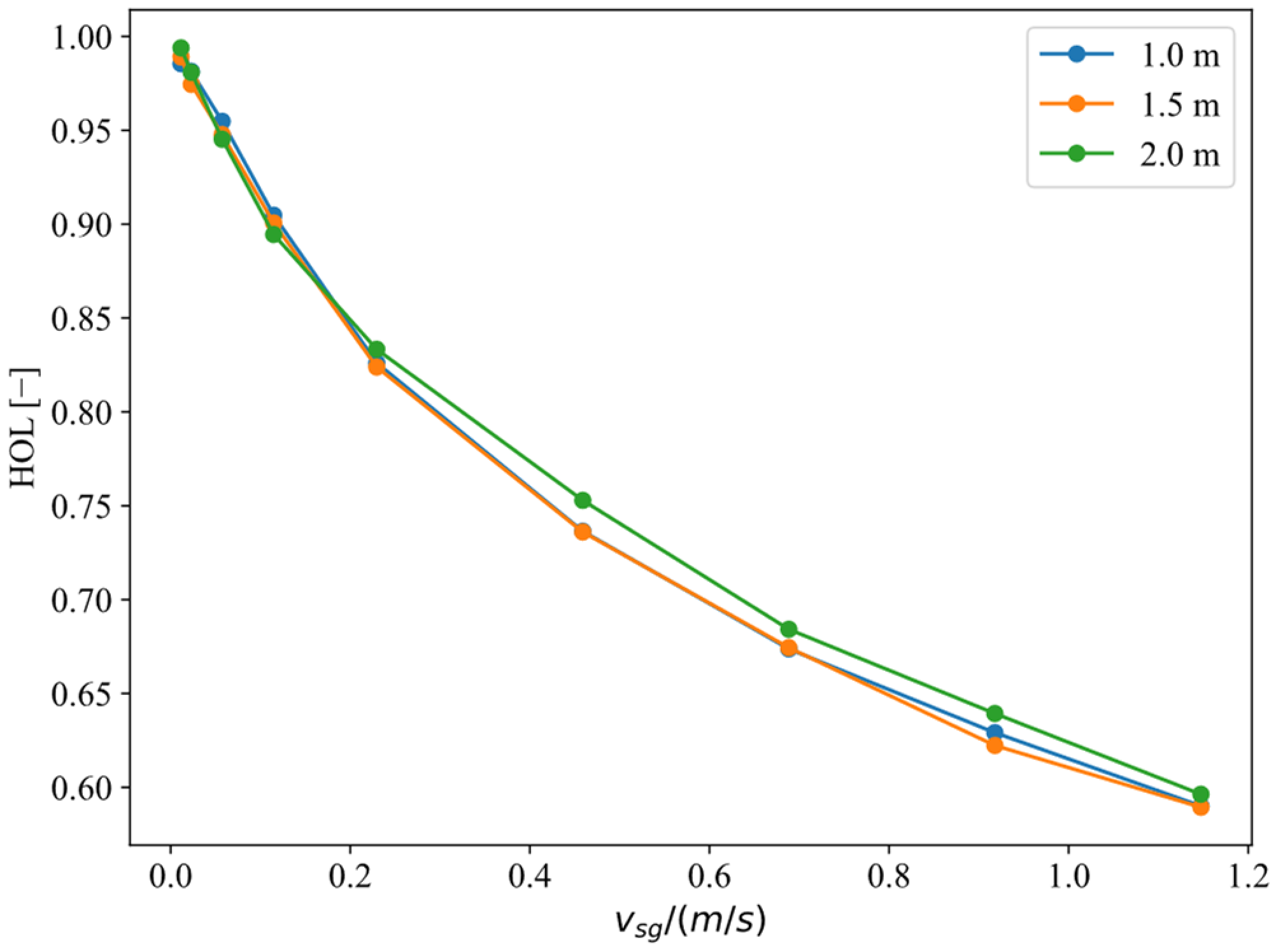
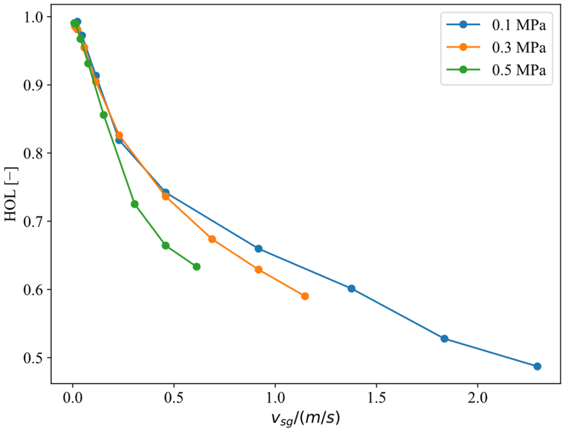
Understanding how casing pressure affects the liquid level in the annulus helps to better control wellbore pressure, prevent blowouts, and ensure operational safety and efficiency. When the wellhead casing pressure increases, the dynamic liquid level in the annulus rises. This is mainly due to the increased casing pressure compressing the gas, requiring a higher liquid column to balance the pressure difference.

(4)

The ZNLF model proposed in this study shows a small error compared to the test data. The flow patterns derived from this model can be used to guide the design of casing pressure and submergence settings for wells with constant pressure gas venting in the annulus.

References

1. Hasan, A.; Kabir, C. Determining Bottomhole Pressures in Pumping Wells. Soc. Pet. Eng. J. 1985, 25, 902–908. [Google Scholar] [CrossRef]
2. Orkiszewski, J. Predicting Two-Phase Pressure Drops in Vertical Pipe. J. Pet. Technol. 1967, 19, 829–838. [Google Scholar] [CrossRef]
3. Aziz, K.; Govier, G. Pressure Drop in Wells Producing Oil and Gas. J. Can. Pet. Technol. 1972, 11, PETSOC-72-03-04. [Google Scholar] [CrossRef]
4. Beggs, D.; Brill, J. An Experimental Study of Two-Phase Flow in Inclined Pipes. J. Pet. Technol. 1973, 25, 607–617. [Google Scholar] [CrossRef]
5. Taitel, Y.; Dukler, A. A Model for Predicting Flow Regime Transitions in Horizontal and near Horizontal Gas-Liquid Flow. AIChE J. 1976, 22, 47–55. [Google Scholar] [CrossRef]
6. Luo, C.; Cao, Y.; Liu, Y.; Zhong, S.; Zhao, S.; Liu, Z.; Liu, Y.; Zheng, D. Experimental and Modeling Investigation on Gas-Liquid Two-Phase Flow in Horizontal Gas Wells. J. Energy Resour. Technol. 2022, 145, 013102. [Google Scholar] [CrossRef]
7. Alqahtani, B.; Alqahtani, M.; Alqahtani, A. Electric Submersible Pump Setting Depth Optimization—A Field Case Study. In Proceedings of the SPE Middle East Artificial Lift Conference and Exhibition, Manama, Bahrain, 25–26 October 2022; OnePetro: Richardson, TX, USA, 2022. [Google Scholar] [CrossRef]
8. Goliatt, L.; Mohammad, R.; Abba, S.; Yaseen, Z. Development of Hybrid Computational Data-Intelligence Model for Flowing Bottom-Hole Pressure of Oil Wells: New Strategy for Oil Reservoir Management and Monitoring. Fuel 2023, 350, 128623. [Google Scholar] [CrossRef]
9. Heinemann, N.; Scafidi, J.; Pickup, G.; Thaysen, E.; Hassanpouryouzband, A.; Wilkinson, M.; Satterley, A.; Booth, M.; Edlmann, K.; Haszeldine, R. Hydrogen Storage in Saline Aquifers: The Role of Cushion Gas for Injection and Production. Int. J. Hydrog. Energy 2021, 46, 39284–39296. [Google Scholar] [CrossRef]
10. Sadatomi, M.; Sato, Y.; Saruwatari, S. Two-Phase Flow in Vertical Noncircular Channels. Int. J. Multiph. Flow 1982, 8, 641–655. [Google Scholar] [CrossRef]
11. Kelessidis, V.C.; Dukler, A.E. Modeling Flow Pattern Transitions for Upward Gas-Liquid Flow in Vertical Concentric and Eccentric Annuli. Int. J. Multiph. Flow 1989, 15, 173–191. [Google Scholar] [CrossRef]
12. Zhu, L.; Ooi, Z.; Zhang, T.; Brooks, C.; Pan, L. Identification of Flow Regimes in Boiling Flow with Clustering Algorithms: An Interpretable Machine-Learning Perspective. Appl. Therm. Eng. 2023, 228, 120493. [Google Scholar] [CrossRef]
13. Caetano, E.; Shoham, O.; Brill, J. Upward Vertical Two-Phase Flow Through an Annulus—Part I: Single-Phase Friction Factor, Taylor Bubble Rise Velocity, and Flow Pattern Prediction. J. Energy Resour. Technol. 1992, 114, 1–13. [Google Scholar] [CrossRef]
14. Salhi, A.; Rey, C.; Rosant, J. Pressure Drop in Single-Phase and Two-Phase Couette-Poiseuille Flow. J. Fluids Eng. 1992, 114, 80–84. [Google Scholar] [CrossRef]
15. Lu, X.; Andrés, L.; Yang, J. A Nonhomogeneous Bulk Flow Model for Gas in Liquid Flow Annular Seals: An Effort to Produce Engineering Results. J. Tribol. 2021, 144, 062302. [Google Scholar] [CrossRef]
16. Liu, A.; Guo, P.; Li, Y.; Liu, H.; Tang, S.; Yang, M.; Zhao, X. Wellbore zero liquid flow study. Oil Drill. Prod. Technol. 2009, 31, 75–78. [Google Scholar]
17. Hasan, A.; Kabir, C. Two-Phase Flow in Vertical and Inclined Annuli. Int. J. Multiph. Flow 1992, 18, 279–293. [Google Scholar] [CrossRef]
18. Liu, L.; Zhou, F. Holdup and pressure drop in tow-phase zero net-liquid flow. J. Eng. Thermophys. 2002, 23, 365–368. [Google Scholar]
19. Liu, L. The Phenomenon of Negative Frictional Pressure Drop in Vertical Two-Phase Flow. Int. J. Heat Fluid Flow 2014, 45, 72–80. [Google Scholar] [CrossRef]
20. Guan, C.; Zhao, G.; Zhang, Y.; Tao, J.; Zhu, L. Calculation method of multi-phase flow and optimization sub-mergence depth of electric pump in casing annulus gas-venting wells. Acta Pet. Sin. 2010, 31, 152–156. [Google Scholar]
21. Wei, N.; Meng, Y.; Liu, Y.; Li, G.; Liu, A. Zero-flow airlift simulation experiment and drawdown law study on under-balanced drilling. Chin. J. Appl. Mech. 2010, 27, 549–552+646. [Google Scholar]
22. Daraboina, N.; Chi, Y.; Sarica, C.; Pereyra, E.; Scott, S. Effects of High Pressure on the Performance of Existing Two-Phase Flow Models in Wellbores. In Proceedings of the SPE Annual Technical Conference and Exhibition, Dallas, TX, USA, 24–26 September 2018; OnePetro: Richardson, TX, USA, 2018. [Google Scholar] [CrossRef]
23. Hasan, A.; Kabir, C.; Rahman, R. Predicting Liquid Gradient in a Pumping-Well Annulus. SPE Prod. Eng. 1988, 3, 113–120. [Google Scholar] [CrossRef]
24. Sun, T.; Zhang, X.; Liu, S.; Cao, Y.; Xie, R. Annular Pressure Buildup Calculation When Annulus Contains Gas. Chem. Technol. Fuels Oils 2018, 54, 484–492. [Google Scholar] [CrossRef]
25. Godbey, J.; Dimon, C. The Automatic Liquid Level Monitor for Pumping Wells. J. Pet. Technol. 1977, 29, 1019–1024. [Google Scholar] [CrossRef]
26. Ding, L.; Yang, X.; Chen, W.; Li, S.; Zhang, Q. Prediction of Annulus Liquid Level Depth in High-Temperature and High-Pressure Gas Wells Based on Sustained Casing Pressure. Measurement 2022, 193, 110991. [Google Scholar] [CrossRef]
27. Arpandi, I.; Joshi, A.; Shoham, O.; Shirazi, S.; Kouba, G. Hydrodynamics of Two-Phase Flow in Gas-Liquid Cylindrical Cyclone Separators. SPE J. 1996, 1, 427–436. [Google Scholar] [CrossRef]
28. Xue, J.; Luo, W.; Liu, Z.; Wu, Z.; Wang, J.; Liao, R. A Criterion of Negative Frictional Pressure Drop in Vertical Two-Phase Flow. Chem. Eng. Trans. 2018, 66, 415–420. [Google Scholar] [CrossRef]
29. Harmathy, T. Velocity of Large Drops and Bubbles in Media of Infinite or Restricted Extent. AIChE J. 1960, 6, 281–288. [Google Scholar] [CrossRef]
30. Jasim, A.; Sultan, A.; Al-Dahhan, M. Influence of Heat-Exchanging Tubes Diameter on the Gas Holdup and Bubble Dynamics in a Bubble Column. Fuel 2019, 236, 1191–1203. [Google Scholar] [CrossRef]
31. Wang, X.; Liu, X.; Zhou, C.; He, H.; Zhang, R. Gas-Liquid Separation Mechanism of Downhole Pump under High Gas Content Condition and Its System Design Method. China Pet. Mach. 2020, 48, 75–80. [Google Scholar] [CrossRef]
32. Zuber, N.; Findlay, J. Average Volumetric Concentration in Two-Phase Flow Systems. J. Heat Transf. 1965, 87, 453–468. [Google Scholar] [CrossRef]
33. Gregory, G.; Scott, D. Correlation of Liquid Slug Velocity and Frequency in Horizontal Cocurrent Gas-Liquid Slug Flow. AIChE J. 1969, 15, 933–935. [Google Scholar] [CrossRef]
34. Wang, W.; Cui, G.; Chen, J.; Xiao, Y. Experiments and Modelling for Predicting Critical Gas Velocity with Zero Net Liquid Flow in Slightly Inclined Pipes. J. Eng. Thermophys. 2020, 41, 3068–3076. [Google Scholar]
35. An, H.; Langlinais, J.; Scott, S. Effects of Density and Viscosity in Vertical Zero Net Liquid Flow. J. Energy Resour. Technol. 2000, 122, 49–55. [Google Scholar] [CrossRef]
Figure 1. Schematic diagram of the experimental setup and process.
Processes 12 01311 g001
Figure 2. (a) Bubble flow; (b) transition from bubble flow to churn flow; (c) churn flow.
Processes 12 01311 g002
Figure 3. Change in dynamic liquid level with vsg at 0.3 MPa.
Processes 12 01311 g003
Figure 4. Change in dynamic liquid level with vsg at an initial liquid column height of 1 m.
Processes 12 01311 g004
Figure 5. Change in holdup with vsg at 0.3 MPa.
Processes 12 01311 g005
Figure 6. Change in holdup with vsg at an initial liquid column height of 1 m.
Processes 12 01311 g006
Figure 7. Change in pressure gradient with vsg at 0.3 MPa.
Processes 12 01311 g007
Figure 8. Change in frictional pressure gradient with vsg at 0.3 MPa.
Processes 12 01311 g008
Figure 9. Physical model of bubble flow.
Processes 12 01311 g009
Figure 10. Churn flow physics model.
Processes 12 01311 g010
Figure 11. Change in holdup with vsg at an initial liquid column height of 2 m.
Processes 12 01311 g011
Figure 12. Change in pressure gradient with vsg.
Processes 12 01311 g012