Article

A Novel Data Mining Framework to Investigate Causes of Boiler Failures in Waste-to-Energy Plants

1
Department of Water Management, Faculty of Civil Engineering and Geosciences, Delft University of Technology, 2628 CN Delft, The Netherlands
2
Department of Computing Science, Umeå University, SE-901 87 Umeå, Sweden
3
Umeå Energi, SE-901 05 Umeå, Sweden
4
Department of Chemistry, Umeå University, SE-907 36 Umeå, Sweden
*
Author to whom correspondence should be addressed.
Processes 2024, 12(7), 1346; https://doi.org/10.3390/pr12071346
Submission received: 15 May 2024 / Revised: 18 June 2024 / Accepted: 21 June 2024 / Published: 28 June 2024

Abstract

:
Examining boiler failure causes is crucial for thermal power plant safety and profitability. However, traditional approaches are complex and expensive, lacking precise operational insights. Although data-driven approaches hold substantial potential in addressing these challenges, there is a gap in systematic approaches for investigating failure root causes with unlabeled data. Therefore, we proffered a novel framework rooted in data mining methodologies to probe the accountable operational variables for boiler failures. The primary objective was to furnish precise guidance for future operations to proactively prevent similar failures. The framework was centered on two data mining approaches, Principal Component Analysis (PCA) + K-means and Deep Embedded Clustering (DEC), with PCA + K-means serving as the baseline against which the performance of DEC was evaluated. To demonstrate the framework’s specifics, a case study was performed using datasets obtained from a waste-to-energy plant in Sweden. The results showed the following: (1) The clustering outcomes of DEC consistently surpass those of PCA + K-means across nearly every dimension. (2) The operational temperature variables T-BSH3rm, T-BSH2l, T-BSH3r, T-BSH1l, T-SbSH3, and T-BSH1r emerged as the most significant contributors to the failures. It is advisable to maintain the operational levels of T-BSH3rm, T-BSH2l, T-BSH3r, T-BSH1l, T-SbSH3, and T-BSH1r around 527 °C, 432 °C, 482 °C, 338 °C, 313 °C, and 343 °C respectively. Moreover, it is crucial to prevent these values from reaching or exceeding 594 °C, 471 °C, 537 °C, 355 °C, 340 °C, and 359 °C for prolonged durations. The findings offer the opportunity to improve future operational conditions, thereby extending the overall service life of the boiler. Consequently, operators can address faulty tubes during scheduled annual maintenance without encountering failures and disrupting production.

1. Introduction

A boiler is an essential component in thermal power plants that utilize various fuels, including coal, oil, nuclear, or waste. Functioning as heat exchangers, boilers transform purified water into high-pressure steam through heat radiation from hot flue gas. This steam subsequently drives turbine blades for electricity generation. Typically, a boiler comprises economizers, evaporators, superheaters, and a steam drum, although the specific configuration may vary depending on the design and function of the power plant [1,2,3,4]. Given the harsh operating conditions of elevated temperature, pressure, corrosive substances, and mechanical stress, boilers are prone to frequent failures. Boiler tube failures account for the majority of unplanned shutdowns in power plants [5]. These failures commonly manifest as tube ruptures, significantly compromising both the safety and revenue of a power plant. In the event of tube rupture, the steam generation process can be halted, or worse, it might lead to more serious accidents, compelling a complete plant shutdown for necessary repairs [6,7,8,9]. Such unplanned downtime leads to substantial economic ramifications for the plant. Research indicates that the average cost of a single day of unscheduled power plant downtime in Europe is approximately EUR 100,000 [10].
Investigating the causes of boiler failures holds significant importance for the safety and profitability of power plants. Extensive research has been dedicated to probing the origins of boiler failures, with a predominant focus on chemical and physical mechanisms. These culprits can be generally classified into several categories, including short-term overheating, long-term overheating (high-temperature creep), caustic corrosion from the water/steam side, hydrogen attack from the water/steam side, high-temperature corrosion from the fireside, and dew point corrosion from the fireside [11,12,13,14,15,16]. These phenomena often occur concurrently and can be intricately interconnected. For example, caustic corrosion can set the stage for hydrogen attack. When substantial quantities of alkaline compounds deposit on the inner surface of a tube, they initiate a reaction with the oxide layer, resulting in the depletion of it. Consequently, the hydroxide ions continue to interact with the inner material of the tube, leading to caustic corrosion. Simultaneously, atomic hydrogen is generated. The atomic hydrogen diffuses into the tube wall, where it reacts with metal carbide, forming methane. The accumulation of methane can result in the formation of cracks in the tube wall, a phenomenon known as hydrogen attack [5]. However, if the oxide layer remains intact and accumulates gradually over time, it can diminish heat exchange between the water/steam and flue gas. This reduction in heat exchange fosters localized overheating, which can significantly contribute to tube creep or fatigue [17,18].
Inspecting failed tubes typically demands complex chemical treatments and expensive equipment, such as Scanning Electron Microscopes [12,19]. Furthermore, findings from one part of the boiler may not be relevant to another due to variations in design and operating conditions among different sections of the boiler. Even for the same boiler component, conclusions may not apply consistently over time, given the dynamic nature of the surrounding environment. For example, variations in fuel mixtures can introduce fluctuations in the environment around the boiler, a common occurrence in waste-to-energy (WtE) plants where the quality of municipal solid waste is uncontrollable [20,21]. Furthermore, some studies indicate that prior corrosion experiences can influence the current rate of corrosion [22].
The ultimate objective of uncovering the root causes of failures is to leverage these insights to inform future operations and proactively prevent similar incidents. Unfortunately, conventional examination methods struggle to pinpoint the exact parameters and their specific values that contributed to the failure. The conventional examination results typically yield general recommendations on adjusting operating conditions, but these fall short of offering precise guidance to operators. Regarding operational guidance, an efficient approach to failure investigation should prioritize the connection between a failure and precise operating parameters without delving extensively into the intricacies of the failure mechanism, especially considering the intricate and variable nature of the aforementioned boiler failure mechanisms. Therefore, it is advisable to harness historical operational monitoring data and apply suitable data science methodologies for failure analysis.
Only very few data science applications related to boilers in power plants have been documented in the literature. For instance, one study demonstrated the high effectiveness of a data-driven approach comprising Wavelet Packet Transform analysis and Deep Neural Network in detecting boiler tube leakages [23]. Another developed two short-term forecasting models (Convolutional Neural Network (CNN) and Long Short-Term Memory Network) for predicting three safety indicators of a supercharged boiler. Both models yielded excellent results, but CNN was preferred due to its lower computational cost [24]. Additionally, an Extreme Gradient Boosting model, fine-tuned with a Particle Swarm Optimization algorithm, accurately predicted the metal temperature time series, enabling the early detection of metal temperature anomalies in a coal-fired boiler [25]. Furthermore, the Extra-Tree classifier and Minimum Redundancy Maximum Relevance model were found to be highly effective in selecting the most relevant sensors for detecting faults in turbines and boilers, respectively. The results indicated a substantial reduction in the number of sensors needed for fault detection and a significant increase in detection accuracy [26]. Moreover, three individual machine learning algorithms, Random Forest, Lasso, and Support Vector Regression, along with the ensemble model based on them, were employed to forecast boiler faults in a thermal power plant by predicting the key performance indicators of the boiler. The findings indicated that the ensemble model outperformed all three individual models, delivering a highly satisfactory outcome [27].
However, the literature presents two gaps. Firstly, there is a lack of data science applications specifically focused on analyzing root causes of boiler failures. Secondly, all the prior studies are based on supervised learning, which is not suitable for scenarios where operational data lacks clear labels, a common occurrence in engineering settings, including the case study addressed in this research. Motivated by these gaps, this study introduces a novel and methodical framework that integrates engineering expertise with data science methods to investigate the causes of boiler failures and improve future operational practices. Beginning with formulating the boiler failure investigation problem into a data mining problem, the framework encompasses data preprocessing, model building and selection, and result evaluation and analysis, culminating in the provision of precise operational recommendations to prevent future boiler failures. The data science techniques employed predominantly include Discrete Wavelet Transform (DWT), Principal Component Analysis (PCA), K-means clustering, and Deep Embedded Clustering (DEC). This framework is designed and leveraged to achieve the aforementioned objective, which is pinpointing the exact operational parameters and their specific values that contributed to boiler failures so that similar failures in the future can be proactively prevented by adjusting process operations.
This paper is structured as follows. Following this introduction, the subsequent section introduces the case study subject and the datasets used in this research. The case study was conducted on a WtE facility situated in Umeå, Sweden. Its purpose was to demonstrate the details of the framework and validate the framework’s applicability in a real engineering context. The Section 3 that follows presents the framework, the chosen data science techniques, and the rationale behind their adoption. The results derived from the case study and the ensuing discussion are then presented in the subsequent section. Finally, the Section 5 summarizes the key findings of this research.

2. Overview of Umeå Waste-to-Energy Plant and Data Origin

The subject of the case study is the WtE plant located in Umeå, Sweden, operated by Umeå Energi. Umeå WtE plant is a 65 MW Combined Heat and Power (CHP) plant fueled by approximately 50% municipal solid waste and 50% industrial waste. Boasting a waste processing capacity of around 20 t/h, the plant operates roughly 8000 h per year and undergoes an annual scheduled maintenance shutdown.
Illustrated in Figure 1 is the boiler-related layout of the Umeå WtE plant. Waste is introduced through the hopper for incineration on the grate, and the resulting flue gas traverses four flue gas passages until it reaches the flue gas treatment modules. The initial three passages are vertically oriented, primarily relying on radiation for heat transfer, while the fourth passage is horizontal and characterized by convective heat exchange. In the initial three passages, numerous tubes containing water/steam are positioned along the inner walls. These tubes serve dual purposes: functioning as evaporators within the boiler system and acting as safeguards against overheating for the walls. In the fourth passage lies the central segment of the boiler arrangement, consisting of one evaporator unit, three superheater units, another evaporator unit, and three economizer units, arranged from left to right. Within this segment, water/steam typically flows counter to the flue gas to facilitate convective processes. Within the economizers, boiler feed water is raised to a temperature below boiling point under certain water pressure. Concurrently, the flue gas surrounding the economizers achieves the desired (lower) temperature for subsequent flue gas treatment. Following the economizers, the heated water ascends to the uppermost steam drum situated atop the flue gas passages. Subsequently, the water in the steam drum flows through the downcomers to reach the evaporators, where it undergoes a phase transition into wet steam before ascending back to the steam drum. Within the steam drum, a separator works to transform the wet steam into saturated steam. This saturated steam is extracted from the upper section of the steam drum and subsequently undergoes additional heating in the superheaters to attain the status of superheated steam. The superheating process is crucial for optimizing turbine efficiency and ensuring its continued optimal performance.
The entirety of the plant is monitored by numerous online sensors. With the assistance of the engineers at the Umeå WtE plant, 66 of them (presented in Table S1 in Supplementary Material) were identified to possess potential associations with boiler failure occurrences. Consequently, there were 66 variables in the case study datasets. Throughout the case study, a total of three boiler failures were examined, each corresponding to a specific repair stoppage. The timeframes for these stoppages were derived from the log. Closely proximate failures were analyzed collectively, resulting in the investigation of two datasets (as outlined in Table 1). The time spans of the datasets were decided by setting the starting points three to five months (depending on the availability of data) before the initial stoppage. This approach ensured an adequate number of observations for evaluating distinctions between normal and abnormal operational conditions (further elaborated on in Section 3.1). The datasets were obtained at a 30 min resolution through averaging, despite the original data being of a higher resolution. Averaging was employed for two main purposes: noise reduction and, notably, mitigation of the time-lag impact caused by the movement of water, steam, and flue gas.

3. Methodology

3.1. The Framework

The investigation into the causes of boiler failure in this study is primarily grounded in the inference that there are certain abnormal conditions giving rise to the failure, and these abnormal conditions persist until the operators detect the failures and halt the process line. Hence, the primary phase of abnormal conditions ceases around the time of the commencement of stoppage/repair. Preceding the occurrence of abnormal conditions there exists a period characterized by normal operational conditions. Through a comparison of variable values under normal and abnormal conditions, we can identify which variables deviate from the expected behavior and consequently lead to failure.
However, identifying the normal and abnormal periods presents a two-fold challenge. First, the monitored data lack labels, aside from the logging of boiler repair events. Second, the criteria for classifying operational conditions as abnormal may differ from one tube to another and across various time periods, owing to variations in the functions of different tubes and the potential degradation of their properties over time. Thus, to the authors’ best knowledge, case-based unsupervised clustering stands as the sole fitting approach for identifying normal and abnormal periods in this study. The specific method of unsupervised clustering applied in this study is K-means [28].
Figure 2 shows the flowchart of the failure analysis framework in this study. Following the initial data cleansing process, the application of Discrete Wavelet Transform (DWT) served to effectively eliminate any noise stemming from the sensors. Next, embedding techniques were implemented to mitigate noise that may exist among different variables. Importantly, the utilization of embedding also aids in averting the curse of dimensionality [29], as it effectively reduces the dimensionality of the data. This study employed two distinct embedding techniques. The first approach was Principal Component Analysis (PCA), whereas the second approach was a Deep Neural Network (DNN) integrated within the structure of Deep Embedded Clustering (DEC). Following the embedding process, the transformed data were input into K-means, producing the final clustering results. PCA + K-means served as the baseline against which the performance of DEC was evaluated. For PCA + K-means, the developments of PCA and K-means are loosely combined as the information flow is unidirectional from PCA to K-means. Conversely, in DEC, the DNN and K-means are seamlessly connected and trained simultaneously and iteratively. The information flow in DEC is bidirectional: from DNN to K-means, further extending to KL divergence, and reciprocally from KL divergence back to K-means and DNN. Having obtained the initial clustering results that categorized all observations into three distinct clusters, the subsequent task was to determine the identity of each cluster. Initially, the repair cluster (period of stoppage) can be discerned by referencing the operational log, as the log indicates when the boiler underwent repair and subsequently resumed operation. Following this, the contiguous timeframe directly preceding the repair event can be recognized as the cluster indicative of abnormal operating conditions. Finally, the continuous timeframe preceding the cluster of abnormal conditions can be designated as the cluster of normal operating conditions. Once the clusters were identified, an assessment and comparison of the clustering outcomes between PCA + K-means and DEC were conducted from an operational perspective. This evaluation aimed to determine the optimal clustering result. Based on this optimal clustering result, histograms were constructed for each individual variable. The purpose was to scrutinize potential disparity in distribution patterns between clusters under normal and abnormal conditions. To quantify this distribution disparity, the Normalized Peak Shift (NPS) metric was employed. It assesses the normalized shift in peak values (the most frequent values) within two distinct distributions. Variables that displayed a noticeable shift, characterized by NPS values surpassing the threshold of 30%, were identified as contributors to failure occurrences. These identified variables require vigilant monitoring to proactively prevent the recurrence of similar failures. Furthermore, recommendations concerning their values during production were formulated based on observations of their distributions under both normal and abnormal conditions.
In addition to the utilization of data science techniques, the experiential insights contributed by WtE plant engineers held a substantial influence within the framework. The term ‘empirical engineering knowledge’ within the framework pertains to the experiential knowledge garnered by the engineers through their operational and maintenance experiences. This encompasses their specialized engineering expertise in the realms of chemistry and physics. This form of knowledge served as an important complement within this framework, ensuring the data science methodologies were effectively employed to align seamlessly with the study’s objectives. For example, as described in Section 2, the engineers helped to narrow down relevant variables significantly. Moreover, empirical engineering knowledge was sought when setting the noise threshold in the DWT process. More importantly, it was employed to evaluate and compare different clustering results, and, finally, to select the optimal one.

3.2. Discrete Wavelet Transform

Discrete Wavelet Transform (DWT) is a powerful tool for denoising signal data [30]. DWT-based denoising typically comprises three steps: Decomposition, Thresholding, and Reconstruction.
Decomposition: Solve the DWT coefficients from the decomposition expansion of the signal with noise. Given a signal s t , decompose it using DWT to obtain the approximation coefficients c j 0 k and detail coefficients d j k . The decomposition expansion can be expressed as Equation (1):
s t = k c j 0 k φ j 0 , k t + k j = j 0 d j k ψ j , k t
Here, ψ j , k t = 2 j 2 ψ ( 2 j t k ) is the wavelet function, and φ j 0 , k t = 2 j 0 2 φ ( 2 j 0 t k ) is the scaling function associated with the wavelet function. j is the level parameter, and k is the translation parameter.
Thresholding: Keep the detail coefficients associated with the signal as they are, and replace the ones related to noise with zeros. Given the detail coefficients d j k , apply a threshold T to it to suppress the noise. This study adopted the hard thresholding approach that is presented in Equation (2):
d j ~ k = d j k   i f   d j k T 0   i f   d j k < T
Reconstruction: Reconstruct the signal with the modified coefficients. Equation (3) demonstrates the reconstructed and denoised signal s ~ t using the original approximation coefficients c j 0 k and the modified detail coefficients d j ~ k :
s ~ t = k c j 0 k φ j 0 , k t + k j = j 0 d j ~ k ψ j , k t
For the DWT work in this study, we used the Python package PyWavelets (version: 1.1.1) [31]. Specifically, we use the wavedec application programming interface (API) for multilevel decomposition with the arguments ‘db6’ for wavelet and 5 for level.

3.3. Principal Component Analysis

Principal Component Analysis (PCA) yields several principal components (PCs), which are the result of mapping the raw data’s variation space to a new space of lower dimensionality. All the PCs are linear combinations of the original variables, but the PCs are orthogonal to each other. The number of PCs is determined by maximizing the total variation explained by the PCs, while minimizing the noise remaining. Typically, PCA is conducted by calculating the covariance matrix of the original data, which is followed by eigenvalue decomposition of the covariance matrix. The eigenvectors from the decomposition define the directions of the PCs. The eigenvectors are sorted according to their corresponding eigenvalues, and larger eigenvalues represent greater capability of explaining variation by the corresponding PCs [32]. For the PCA work in this study, we used the API sklearn.decomposition.PCA in the Python package sickit-learn (version: 0.24.0) [33].

3.4. K-Means

The idea of K-means clustering is quite straightforward: all the observations in the dataset are grouped into k clusters based on their distances to each other, minimizing the distances among observations within each cluster, while maximizing the distances among different clusters [28]. To be specific, the objective of K-means is to minimize E, as presented in Equation (4):
E = i = 1 k x C i x μ i 2
Here, k is the set number of clusters, C i is the ith cluster, and μ i is the mean vector (centroid) of C i . Since the total variance is constant, minimizing E is equivalent to maximizing the variance among different clusters.
However, minimizing E is an NP-hard problem. Thus, the following heuristic algorithm is used:
(1)
Randomly generate k initial centroids within the dataset.
(2)
Generate new clusters by assigning every observation to its nearest centroid.
(3)
Calculate the centroids of the new clusters.
(4)
Repeat Steps 2 and 3 until convergence is reached.
For the K-means work (for both PCA + K-means and DEC) in this study, we used the Python API sklearn.cluster.KMeans in the Python package sickit-learn (version: 0.24.0) [33] with the parameters n_clusters = 3, tol = 0.001, and random_state = 5. The number of clusters for K-means was set to 3, because for every case, there are three categories of operating conditions for the boiler–normal conditions, abnormal conditions, and repair/stoppage.

3.5. Deep Embedded Clustering

Deep Embedded Clustering (DEC) is a method that learns variable embedding and observation clustering simultaneously using deep neural networks (DNN) and K-means [34]. Instead of clustering the original data X into k clusters, DEC first maps X nonlinearly onto a new space Z with much lower dimensionality. The mapping is conducted through a DNN with the parameters   θ . Subsequently, DEC learns the centroids set μ i Z   i = 1 k and the parameter θ simultaneously. DEC consists of two stages:
(1)
Using a stacked autoencoder (SAE) to initialize the parameters θ .
(2)
Iterating the process of generating an auxiliary target distribution and minimizing the Kullback–Leibler (KL) divergence between the soft assignment q i j and the auxiliary target distribution p i j . By doing this, the parameters θ are optimized.
SAE is applied because much research has demonstrated its capability of consistently yielding good representations (results of mapping) for real-world datasets [35,36,37]. As shown by Figure S1 in Supplementary Material, SAE consists of an encoder and a decoder, and their structures are symmetric with respect to one another. The low-dimension layer in the middle is the embedded space. The activation function applied for the SAE (except for the embedded layer and the reconstruction layer) in this study is ReLU [38]. The training is performed by minimizing the least-square loss between the input layer and the reconstruction layer. Once initialization is carried out, the encoder part is selected to concatenate with K-means in Stage (2) for further training.
In Stage (2), the loss function KL divergence is expressed in Equation (5):
K L ( P Q ) = i j p i j l o g p i j q i j
The term q i j mentioned above is defined in Equation (6):
q i j = 1 + z i μ j 2 α α + 1 2 j 1 + z i μ j 2 α α + 1 2  
Here, z i Z corresponds to x i X , and α are the degrees of freedom of the Student’s t distribution. q i j indicates the probability of assigning sample i to cluster j.
The term p i j mentioned above is defined in Equation (7):
p i j = q i j 2 f j j q i j 2 f j
Here, f j = i q i j are soft cluster frequencies.
The DEC work in this study was carried out based on the Keras script written by Xifeng Guo [39]. The original script was designed to perform image clustering, but we customized it to fit this study.

3.6. Key Hyperparameters of Models

Since the primary focus of this study is the optimization of the WtE process, the description and discussion of the data science methodology are presented concisely. Therefore, only the core hyperparameters of the models are discussed in this paper, while any API arguments not explicitly mentioned are retained at their default settings. We adopted the Grad Student Descent approach [40] for tuning all the model hyperparameters. In our analyses, two key hyperparameters took center stage: the number of PCs (npc) for PCA + K-means, and the number of neurons in the embedded layer (nn_el) for DEC. They both dictate the dimensionality of the embedded spaces. To facilitate optimization, we defined an identical range, specifically {2, 3, 4, 5, 6, 7, 8}, for both of these hyperparameters’ tuning. In cases where the optimal outcome for either approach emerged at 2 or 8, an exploration of 1 or 9 would be initiated to assess the potential for yielding a new optimal result. This iterative process would continue until the superior outcome was no longer derived from the boundary values of the specified range. For DEC, additional significant hyperparameters included the number of hidden layers within the encoder (nhl) and the number of neurons within these layers (nn_hl). Given the datasets’ moderate scales, the optimization range for nhl was designated as {1, 2, 3}, with 2 consistently identified as the optimal selection across all datasets. To enhance tuning efficiency, we maintained uniformity in nn_hl across all hidden layers for a specific dataset. Nevertheless, the optimization ranges and optimal values for nn_hl differed among datasets.

3.7. Normalized Peak Shift

Normalized Peak Shift (NPS) was introduced as the metric to evaluate the state difference of each variable between normal conditions and abnormal conditions. It is based on the notion that the most frequently observed value (peak value of a distribution) under certain conditions can effectively encapsulate the variable’s state under those conditions. Thus, by estimating the peak values’ shift between two distributions, the state change of the variable of interest can be quantified. To enhance the clarity and utility of this metric, the range of variable values under normal conditions (excluding extreme values) is utilized to normalize the shift, resulting in NPS values presented as percentages. N P S can be calculated by Equation (8):
N P S = f x n h x a   max 1 i < j k x n i x n j  
Here, f x n is the Probability Mass Function (PMF) of the variable values under normal conditions ( x n ), while h x a is the PMF of the variable values under abnormal conditions ( x a ). k is the number of observations under normal conditions after excluding the observations with extreme variable values.

4. Results and Discussion

4.1. Results for Dataset A

There are two boiler failures in Dataset A. Within the DEC approach, we defined the optimization range for nn_hl as {70, 80, 90, 100}, determining that 80 emerged as the optimal value. By employing this optimal nn_hl, we obtained the DEC’s optimal clustering outcome when nn_el was set to 2. Within the PCA+K-means approach, we observed that none of the values within the set {1, 2, 3, 4, 5, 6, 7, 8} proved to be an effective npc value that was capable of delineating a distinct separation between the normal conditions cluster and the abnormal conditions cluster. Accordingly, as summarized in Table 2, the optimal clustering result for Dataset A was achieved using DEC with nhl, nn_hl, and nn_el set to 2, 80, and 2, respectively. The optimal clustering result is shown in Figure 3. The complete compilation of results obtained from both DEC and PCA + K-means under various hyperparameter settings can be accessed in Section S3 in the Supplementary Material.
Applying the method expounded in Section 3.1, the three clusters in Figure 3 can be readily identified. Cluster 2 is the repair periods/stoppages caused by the failures since it matches the timelines of repair according to the log information. Consequently, Cluster 1 can be identified as the abnormal conditions directly contributing to the failures, while Cluster 0 is the normal conditions. Based on this clustering result, the NPS values of each variable were calculated. The histograms of the variables displaying substantial disparities between normal and abnormal conditions (NPS > 30%) are demonstrated in Figure 4.
As illustrated in Figure 4, 17 variables exhibit NPS values surpassing 30%. Notably, T-FaG2 demonstrates the highest value at 94.0%, while T-BSH1r records the lowest at 33.8%. The substantial number of involved variables coupled with elevated average NPS values underscores an extensive and noteworthy shift in the state between these two operational conditions. It is noteworthy that the variables T-FaG1 and T-FaG2 correspond to the two temperature sensors in closest proximity to the incineration area, thus their values are expected to be significantly higher compared to others. However, as depicted in Figure 4, a substantial portion of T-FaG2 values is remarkably low (nearing 0) under both normal and abnormal conditions, in contrast to the regular patterns observed in other variables’ values. This observation leads to the inference that the T-FaG2 sensor experienced prolonged malfunction while the data were recorded. Consequently, despite having the highest NPS value among all variables, T-FaG2 is excluded from further consideration and analysis.
Among the variables displayed in Figure 4, all except T-BEM3rl pertain to flue gas temperatures within the superheater area (red modules in Figure 1). This collective observation implies a significant overheating issue across the entirety of the superheater area, which emerges as the most likely culprit behind the failures encountered in Dataset A. The top three variables ranked by their NPS values are T-BSH3rm, T-BSH2l, and T-BSH3r, exhibiting NPS values of 57.2%, 56.7%, and 53.4%, respectively. This signifies that the temperatures of flue gas at “Superheater 3 roof middle”, “Superheater 2 left”, and “Superheater 3 right” deviated considerably from the normal operational temperatures. Therefore, these variables stand out as the primary contributors to the failures observed in Dataset A. Given the adjacency of all three superheaters, the temperatures within the superheater area are naturally linked and interdependent. Thus, prioritizing the management of the top three influential variables has the potential to effectively address the overarching overheating concern throughout the entire superheater area. According to Figure 4, the peak operational values of T-BSH3rm, T-BSH2l, and T-BSH3r during normal conditions were recorded as 527 °C, 432 °C, and 482 °C, respectively. Under abnormal conditions, these values escalated to 594 °C, 471 °C, and 537 °C, correspondingly. To ensure future production safety, it is advisable to maintain the operational levels of T-BSH3rm, T-BSH2l, and T-BSH3r around 527 °C, 432 °C, and 482 °C respectively. Additionally, it is crucial to prevent these values from reaching or exceeding 594 °C, 471 °C, and 537 °C for prolonged durations. Please refer to Section 4.3 for the discussion on the results and underlying mechanisms.

4.2. Results for Dataset B

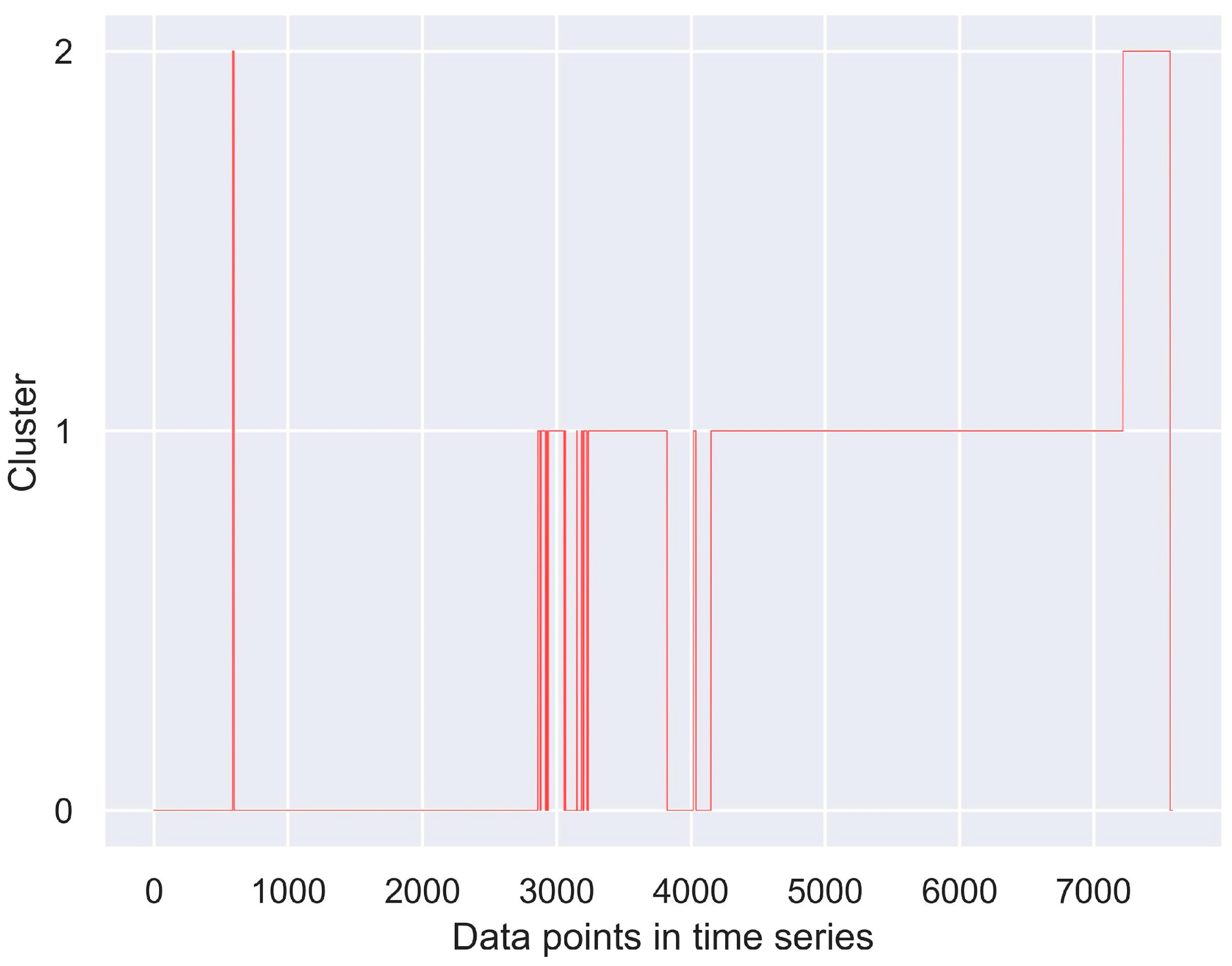
There is one boiler failure in Dataset B. Within the DEC approach, we defined the optimization range for nn_hl as {80, 100, 128, 156}, determining that 128 emerged as the optimal value. By employing this optimal nn_hl, we obtained the DEC’s optimal clustering outcome when nn_el was set to 8. Within the PCA+K-means approach, we observed that none of the values within the set {2, 3, 4, 5, 6, 7, 8, 9} proved to be an effective npc value that was capable of delineating a distinct separation between the normal conditions cluster and the abnormal conditions cluster. Accordingly, as summarized in Table 2, the optimal clustering result for Dataset A was achieved using DEC with nhl, nn_hl, and nn_el set to 2, 128, and 8, respectively. The optimal clustering result is shown in Figure 5. The complete compilation of results obtained from both DEC and PCA + K-means under various hyperparameter settings can be accessed in Section S4 in the Supplementary Material.
Table 2. Optimal hyperparameter values for the DEC models on Datasets A and B.
Dataset IDnhlnn_hlnn_el
A2802
B21288
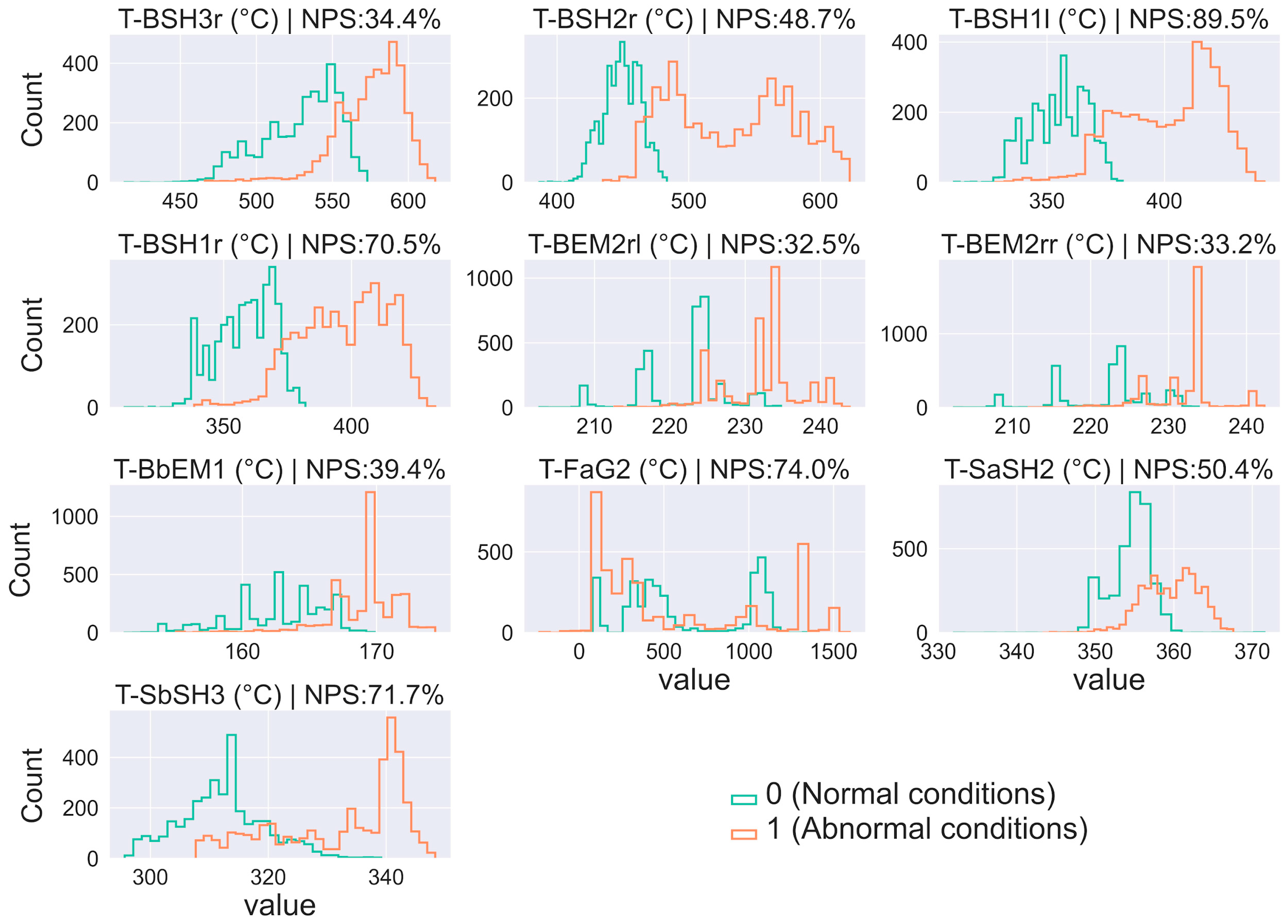
Applying the method expounded in Section 3.1, three distinct clusters can be discerned. Cluster 2 signifies stoppages, Cluster 1 denotes abnormal conditions, and Cluster 0 corresponds to normal conditions. Nevertheless, a brief segment of Cluster 2 is evident within the initial phase of Cluster 0. Engineers at Dåva 1 believed that this occurrence is likely unrelated to the boiler failure, suggesting it may reflect a transient glitch within the monitoring system. Based on this clustering result, the NPS values of each variable were calculated. The histograms of the variables displaying substantial disparities between normal and abnormal conditions (NPS > 30%) are demonstrated in Figure 6.
As illustrated in Figure 6, 10 variables exhibit NPS values surpassing 30%. Notably, T-BSH1l demonstrates the highest value at 89.5%, while T-BEM2rl records the lowest at 32.5%. It is worth noticing that T-FaG2 holds the second-highest NPS value (74.0%) among all the variables. However, the histogram pattern of T-FaG2 closely resembles its counterpart in Dataset A. Consequently, based on the analysis of Dataset A, T-FaG2 is disregarded for subsequent consideration and analysis, despite its elevated NPS value.
In contrast to Dataset A, the variables in Figure 6 comprise a more balanced combination of temperatures from both economizers (green modules in Figure 1) and superheaters. Among them, T-BbEM1, T-BEM2rr, and T-BEM2rl are temperatures within the economizer sector, while the remaining variables pertain to temperatures in the superheater sector. In addition, this implies that the temperature of the evaporator situated between the first superheater and the third economizer likely underwent a comparable shift pattern, despite the absence of a designated sensor for the evaporator. The presence of these variables in Figure 6 suggests an overall overheating of the entire fourth flue gas pass during the abnormal conditions. What resembles Dataset A is the consistent prominence of variables associated with the superheaters. The top three variables for Dataset B ranked by their NPS values are T-BSH1l, T-SbSH3, and T-BSH1r, recording NPS values of 89.5%, 71.7%, and 70.5% respectively. They are the temperatures of flue gas at “Superheater 1 left”, steam prior to “Superheater 3”, and flue gas at “Superheater 1 right”. Additionally, T-SaSH2 and T-BSH2r exhibit noteworthy NPS values of 50.4% and 48.7%, respectively, ranking as the fourth and fifth most influential variables. Importantly, all five variables correspond to either flue gas or steam temperatures within the superheater area, signifying an intensified overheating specifically concentrated in the superheater region within the already overheated fourth flue gas pass. Thus, these variables emerge as the primary causative factors behind the failure observed in Dataset B. Given the linkage and interdependence between the temperatures in the fourth flue gas pass, prioritizing the management of the top three influential variables has the potential to effectively address the overheating concern throughout the entire fourth flue gas pass. According to Figure 6, the peak operational values of T-BSH1l, T-SbSH3, and T-BSH1r during normal conditions were recorded as 356 °C, 313 °C, and 368 °C, respectively. Under abnormal conditions, these values escalated to 412 °C, 340 °C, and 408 °C, correspondingly. It is worth noting that T-BSH1l and T-BSH1r were also recognized as significant contributors to the failures in Dataset A (see Figure 4), despite not being part of the top three ranked variables. In Dataset A, their respective peak values during normal conditions were 338 °C and 343 °C, while during abnormal conditions, these values increased to 355 °C and 359 °C. Consequently, to uphold the highest safety standards, it is advisable to maintain the operational levels of T-BSH1l, T-SbSH3, and T-BSH1r around 338 °C, 313 °C, and 343 °C, respectively. Additionally, it is crucial to prevent these values from reaching or exceeding 355 °C, 340 °C, and 359 °C for prolonged durations. Please refer to Section 4.3 for the discussion on the results and underlying mechanisms.

4.3. Discussion on the Results and Underlying Mechanisms

Four types of operational variables—temperature, pressure, chemical concentration, and fluid flow rate—were investigated in this study. Among these, the results illustrated that elevated temperatures, particularly those in close proximity to both inside and outside of superheaters, emerge as the predominant cause for boiler failures. This observation aligns with numerous prior investigations into boiler failure, which employed conventional chemical and physical methodologies. Engineers and researchers widely acknowledge that elevated temperatures can directly result in the rupture of boiler pipes or expedite the occurrence of such ruptures.
For example, thermal fatigue is prevalent with boilers. Thermal fatigue arises when metal components undergo substantial fluctuations in temperature, particularly during repetitive cycles of heating and cooling. These fluctuations can lead to substantial variations in thermal expansion among the structural elements. Depending on the magnitude of the thermal shock experienced, failure may manifest within a few cycles. This process induces multiaxial stresses on the affected surfaces, giving rise to microcracks along the pipe’s surface. Once initiated, these cracks continue to propagate with each subsequent cycle [41,42,43]. Hence, it is imperative to avert situations that introduce significant temperature fluctuations, such as frequent adjustments to burner settings, inconsistent fuel supply, or excessive on/off cycles.
Overheating is another significant temperature-related cause of boiler failures, which encompasses both short-term and long-term overheating. The short-term overheating problem occurs when pipes experience elevated temperatures and insufficient cooling, often causing the pipe temperature to exceed the eutectoid transformation temperature of the pipe materials. Moreover, the rise in material temperature can induce a significant escalation of stress within the pipe, potentially surpassing the pipe’s yield point. The short-term overheating problem can be triggered by factors like water/steam deprivation, flow stagnation due to blockages, uneven flame temperature, etc. [44,45,46].
Conversely, long-term overheating transpires over an extended duration, as the term implies. Long-term overheating problems have been reported as the most common cause of boiler failures [47,48,49]. The continuous exposure to elevated temperatures, often surpassing intended or recommended operational thresholds, can result in the deterioration of the pipes’ microstructure, characterized by phenomena such as graphitization and spheroidization. Along with the constant stress on the pipes, this gradually leads to a slow, time-dependent deformation (creep) and eventually the rupture of the pipes [50,51,52]. Long-term overheating may manifest as a result of various underlying factors, including inadequate circulation, scaling, and flame impingement [53,54]. For instance, the presence of scales on the interior surface of pipes can contribute to the occurrence or exacerbation of long-term overheating issues. The low thermal conductivity of scales results in the potential evaporation of water beneath them when exposed to excessive heat. This process of evaporation can progressively elevate the pH of the water to a critical point, thereby fostering conditions conducive to localized caustic corrosion or embrittlement. Ultimately, this sequence of events culminates in the eventual failure of the boiler [55,56,57].

4.4. Factors Contributing to DEC’s Superior Performance over PCA + K-Means

As can be seen in Sections S3 and S4 of the Supplementary Material, the clustering outcomes achieved by DEC consistently surpass those of PCA + K-means across nearly every dimension. This discrepancy in performance can be attributed to the mechanisms inherent in these two methods. PCA + K-means comprises transforming the original variable space through linear PCA embedding, followed by K-means clustering in the transformed space. Conversely, DEC utilizes an encoder module (DNN) extracted from a pre-trained SAE for embedding, enabling simultaneous, iterative training of DNN and K-means bidirectionally. The DNN forwards the embedded information to K-means clustering, further extending to KL divergence. Reciprocally, DNN and K-means receive feedback from KL divergence for optimization, creating a seamless and iterative process. To be more specific, the DEC system involves iterative refinement of the non-linearly embedded space and cluster centroids based on KL divergence feedback. In contrast, the PCA + K-means approach utilizes linear embedding and lacks iterative feedback optimization. Furthermore, DEC benefits from a wider array of tunable core hyperparameters (such as nhl and nn_hl), whereas PCA + K-means is limited to npc alone.

4.5. Significance of Study and Limitations

As mentioned in the Section 1, this study focuses on an operational-parameter-oriented investigation of failure causes, rather than an exhaustive examination of intricate physical or chemical mechanisms. The objective is not to pinpoint precise physical or chemical reactions leading to failures, but rather to optimize future operational conditions for the purpose of prolonging the boiler’s overall service life. Through this approach, operators can address faulty tubes during scheduled annual maintenance without encountering failures and disrupting production. The notable benefit of this study is its accessibility to operators, as the outcomes are straightforward, encompassing solely operational parameters and their recommended values. Informed by the findings, operators can adjust the production process as needed to ensure that the operating parameters remain within a secure range. This failure investigation framework is applicable not only to WtE plants but also potentially to any production line characterized by numerous operating parameters, even when lacking operating-condition labels in the data.
As aforementioned in Section 4.3, elevated temperature-induced mechanisms are the primary causes of failures studied in this case study. However, precisely identifying the specific mechanisms responsible for the failures is beyond the scope of this research, as outlined in the Section 1. Various mechanisms can intertwine and interact, contributing to the occurrence of failures. Given this complexity, extensive additional research and traditional examination approaches are necessary, rather than relying solely on data-driven methods.
The variables identified as culprits in the investigation of failures—specifically, elevated flue gas and steam temperatures—directly triggered cracking, bulging, or bursting. However, various other factors might also have played a role in the eventual failures, including long-term corrosion, physical stress or impact, and oxidation, which are beyond the scope of this study’s findings. Monitoring some of these parameters might not be feasible, resulting in unavailable data. Alternatively, for other parameters, relevant factors were monitored, such as the concentration of acidic compounds (SO2, HCl, etc.) known to contribute to corrosion. The impact of these acidic compounds is usually not immediately significant but rather accumulates gradually over time, implying that data collected within a specific period may not accurately capture their true influence. This deduction has been substantiated by the fact that none of the variables relating to acidic compounds was identified as influential for the failures.

5. Conclusions

A novel and methodical data mining framework was introduced for conducting operational-level (focused on operating parameters) investigations into the attribution of boiler failures. The framework centered on two data mining approaches, PCA + K-means and DEC, with PCA + K-means serving as the baseline against which the performance of DEC was evaluated. To demonstrate the framework’s specifics, a case study was performed using datasets obtained from a WtE plant in Sweden. Within the case study, different operational conditions were clustered and identified, followed by the quantification of shifts in variable states between normal and abnormal conditions. Based on this quantification, we pinpointed the variables that played a substantial role in causing failures and recommended their safe operational values to forestall similar incidents in the future. The major findings of the case study are as follows:
(1)
The clustering outcomes of DEC consistently surpass those of PCA + K-means across nearly every dimension. This is attributed to DEC’s iterative refinement of the non-linearly embedded space and cluster centroids based on KL divergence feedback.
(2)
T-BSH3rm, T-BSH2l, T-BSH3r, T-BSH1l, T-SbSH3, and T-BSH1r emerged as the most significant contributors to the three failures recorded in the two datasets. This underscores the critical importance of vigilant monitoring and precise temperature control of the superheaters to ensure safe production.
(3)
It is advisable to maintain the operational levels of T-BSH3rm, T-BSH2l, T-BSH3r, T-BSH1l, T-SbSH3, and T-BSH1r around 527 °C, 432 °C, 482 °C, 338 °C, 313 °C, and 343°C, respectively. Additionally, it is crucial to prevent these values from reaching or exceeding 594 °C, 471 °C, 537 °C, 355 °C, 340 °C, and 359 °C for prolonged durations.
The findings offer the opportunity to improve future operational conditions, thereby extending the overall service life of the boiler. Consequently, operators can address faulty tubes during scheduled annual maintenance without encountering failures and disrupting production. In future research, by examining a broader range of failures, we can develop a repository of diverse influential variables and their recommended operational values. This resource can facilitate more comprehensive, precise, and reliable production operation and management.

Supplementary Materials

The following supporting information can be downloaded at: https://www.mdpi.com/article/10.3390/pr12071346/s1, Table S1: List of failure-related operational variables with full name, short name, and unit, of each; Figure S1: DEC structure; Figure S2: Complete clustering results for PCA+K-means for dataset A; Figure S3: Complete clustering results for DEC for dataset A; Figure S4: Complete clustering results for PCA+K-means for dataset B; Figure S5: Complete clustering results for DEC for dataset B.

Author Contributions

Conceptualization, D.W., M.K., E.W. and M.T.; Methodology, D.W.; Validation, D.W., L.J., M.K., E.W. and J.T.; Formal analysis, D.W.; Investigation, D.W., M.K., E.W. and M.T.; Resources, J.T. and M.T.; Data curation, D.W., M.K. and E.W.; Writing—original draft, D.W.; Writing—review & editing, D.W., L.J., J.T. and M.T.; Visualization, D.W.; Supervision, L.J., J.T. and M.T.; Project administration, J.T. and M.T.; Funding acquisition, M.T. All authors have read and agreed to the published version of the manuscript.

Funding

This research received no external funding.

Data Availability Statement

The data presented in this study are not publicly available due to commercial restrictions.

Acknowledgments

The present work was performed as part of the Green Technology and Environmental Economics Research and Collaboration Platform (Green TEE) at Umeå University. Green TEE is a collaborative interface between municipal companies and academic researchers directed toward improving the sustainable performance of cities. The authors acknowledge support from the Green TEE platform for performing this project. The authors would also like to acknowledge support from Umeå Energi, Umeå, Sweden, in organizing study visits and providing the data required in order to perform this study.

Conflicts of Interest

Authors Måns Kjellander and Eva Weidemann were employed by the company Umeå Energi. All authors declare that the research was conducted in the absence of any commercial or financial relationships that could be construed as a potential conflict of interest.

Nomenclature

APIApplication Programming Interface
DECDeep Embedded Clustering
DMData Mining
DNNDeep Neural Network
DWTDiscrete Wavelet Transform
HFHigh-pass Filter
IDInduced Draft
KLKullback–Leibler
LFLow-pass Filter
nhlnumber of hidden layers of the encoder
nn_elnumber of neurons in the embedded layer of DEC
nn_hlnumber of neurons in the hidden layer of DEC
npcnumber of PCs
PCPrincipal Component
PCAPrincipal Component Analysis
PMFProbability Mass Function
SAEStacked Autoencoder
WtEWaste-to-Energy

References

  1. Agarwal, S.; Suhane, A. Study of boiler maintenance for enhanced reliability of system A review. Mater. Today Proc. 2017, 4, 1542–1549. [Google Scholar] [CrossRef]
  2. Barma, M.; Saidur, R.; Rahman, S.; Allouhi, A.; Akash, B.; Sait, S.M. A review on boilers energy use, energy savings, and emissions reductions. Renew. Sustain. Energy Rev. 2017, 79, 970–983. [Google Scholar] [CrossRef]
  3. Liu, J.; Zhao, J.; Zhu, Q.; Huo, D.; Li, Y.; Li, W. Methanol-based fuel boiler: Design, process, emission, energy consumption, and techno-economic analysis. Case Stud. Therm. Eng. 2024, 54, 103885. [Google Scholar] [CrossRef]
  4. Elwardany, M. Enhancing Steam Boiler Efficiency through Comprehensive Energy and Exergy Analysis: A Review. Process Saf. Environ. Prot. 2024, 184, 1222–1250. [Google Scholar] [CrossRef]
  5. Saha, A. Boiler tube failures: Some case studies. In Handbook of Materials Failure Analysis with Case Studies from the Chemicals, Concrete and Power Industries; Elsevier: Amsterdam, The Netherlands, 2016; pp. 49–68. [Google Scholar]
  6. Kumar, S.; Kumar, M.; Handa, A. Combating hot corrosion of boiler tubes—A study. Eng. Fail. Anal. 2018, 94, 379–395. [Google Scholar] [CrossRef]
  7. Shokouhmand, H.; Ghadimi, B.; Espanani, R. Failure analysis and retrofitting of superheater tubes in utility boiler. Eng. Fail. Anal. 2015, 50, 20–28. [Google Scholar] [CrossRef]
  8. Xue, S.; Guo, R.; Hu, F.; Ding, K.; Liu, L.; Zheng, L.; Yang, T. Analysis of the causes of leakages and preventive strategies of boiler water-wall tubes in a thermal power plant. Eng. Fail. Anal. 2020, 110, 104381. [Google Scholar] [CrossRef]
  9. Hu, W.; Xue, S.; Gao, H.; He, Q.; Deng, R.; He, S.; Xu, M.; Li, Z. Leakage failure analysis on water wall pipes of an ultra-supercritical boiler. Eng. Fail. Anal. 2023, 154, 107670. [Google Scholar] [CrossRef]
  10. Baglee, D.; Gorostegui, U.; Jantunen, E.; Sharma, P.; Campos, J. How can SMEs adopt a new method to advanced maintenance strategies? A Case study approach. In Proceedings of the COMADEM 2017 30th International Congress & Exhibition on Condition Monitoring and Diagnostic Engineering Management, Lancashire, UK, 10–13 July 2017. [Google Scholar]
  11. Ichihara, T.; Koike, R.; Watanabe, Y.; Amano, Y.; Machida, M. Hydrogen damage in a power boiler: Correlations between damage distribution and thermal-hydraulic properties. Eng. Fail. Anal. 2023, 146, 107120. [Google Scholar] [CrossRef]
  12. Haghighat-Shishavan, B.; Firouzi-Nerbin, H.; Nazarian-Samani, M.; Ashtari, P.; Nasirpouri, F. Failure analysis of a superheater tube ruptured in a power plant boiler: Main causes and preventive strategies. Eng. Fail. Anal. 2019, 98, 131–140. [Google Scholar] [CrossRef]
  13. Ding, Q.; Tang, X.-F.; Yang, Z.-G. Failure analysis on abnormal corrosion of economizer tubes in a waste heat boiler. Eng. Fail. Anal. 2017, 73, 129–138. [Google Scholar] [CrossRef]
  14. Mudgal, D.; Ahuja, L.; Bhatia, D.; Singh, S.; Prakash, S. High temperature corrosion behaviour of superalloys under actual waste incinerator environment. Eng. Fail. Anal. 2016, 63, 160–171. [Google Scholar] [CrossRef]
  15. Pal, U.; Kishore, K.; Mukhopadhyay, S.; Mukhopadhyay, G.; Bhattacharya, S. Failure analysis of boiler economizer tubes at power house. Eng. Fail. Anal. 2019, 104, 1203–1210. [Google Scholar] [CrossRef]
  16. Pramanick, A.; Das, G.; Das, S.K.; Ghosh, M. Failure investigation of super heater tubes of coal fired power plant. Case Stud. Eng. Fail. Anal. 2017, 9, 17–26. [Google Scholar] [CrossRef]
  17. Jones, D. Creep failures of overheated boiler, superheater and reformer tubes. Eng. Fail. Anal. 2004, 11, 873–893. [Google Scholar] [CrossRef]
  18. Kain, V.; Chandra, K.; Sharma, B. Failure of carbon steel tubes in a fluidized bed combustor. Eng. Fail. Anal. 2008, 15, 182–187. [Google Scholar] [CrossRef]
  19. Guo, H.; Fan, W.; Liu, Y.; Long, J. Experimental investigation on the high-temperature corrosion of 12Cr1MoVG boiler steel in waste-to-energy plants: Effects of superheater operating temperature and moisture. Process Saf. Environ. Prot. 2024. [Google Scholar] [CrossRef]
  20. Gu, B.; Jiang, S.; Wang, H.; Wang, Z.; Jia, R.; Yang, J.; He, S.; Cheng, R. Characterization, quantification and management of China’s municipal solid waste in spatiotemporal distributions: A review. Waste Manag. 2017, 61, 67–77. [Google Scholar] [CrossRef] [PubMed]
  21. Tsiliyannis, C.A. Enhanced waste to energy operability under feedstock uncertainty by synergistic flue gas recirculation and heat recuperation. Renew. Sustain. Energy Rev. 2015, 50, 1320–1337. [Google Scholar] [CrossRef]
  22. Paz, M.; Zhao, D.; Karlsson, S.; Liske, J.; Jonsson, T. Investigating corrosion memory: The influence of previous boiler operation on current corrosion rate. Fuel Process. Technol. 2017, 156, 348–356. [Google Scholar] [CrossRef]
  23. Sohaib, M.; Kim, J.-M. Data driven leakage detection and classification of a boiler tube. Appl. Sci. 2019, 9, 2450. [Google Scholar] [CrossRef]
  24. Jia, X.; Sang, Y.; Li, Y.; Du, W.; Zhang, G. Short-term forecasting for supercharged boiler safety performance based on advanced data-driven modelling framework. Energy 2022, 239, 122449. [Google Scholar] [CrossRef]
  25. Cui, Z.; Xu, J.; Liu, W.; Zhao, G.; Ma, S. Data-driven modeling-based digital twin of supercritical coal-fired boiler for metal temperature anomaly detection. Energy 2023, 278, 127959. [Google Scholar] [CrossRef]
  26. Khalid, S.; Hwang, H.; Kim, H.S. Real-world data-driven machine-learning-based optimal sensor selection approach for equipment fault detection in a thermal power plant. Mathematics 2021, 9, 2814. [Google Scholar] [CrossRef]
  27. Qin, H.; Yin, S.; Gao, T.; Luo, H. A data-driven fault prediction integrated design scheme based on ensemble learning for thermal boiler process. In Proceedings of the 2020 IEEE International Conference on Industrial Technology (ICIT), Buenos Aires, Argentina, 26–28 February 2020; pp. 639–644. [Google Scholar]
  28. Jain, A.K. Data clustering: 50 years beyond K-means. Pattern Recognit. Lett. 2010, 31, 651–666. [Google Scholar] [CrossRef]
  29. Verleysen, M.; François, D. The curse of dimensionality in data mining and time series prediction. In Proceedings of the International work-conference on artificial neural networks, Barcelona, Spain, 8–10 June 2005; pp. 758–770. [Google Scholar]
  30. Burrus, S.; Burrus, C.S.; Gopinath, R.A.; Guo, H.; Odegard, J.A.N.E.A.; Selesnick, I.W.A. Introduction to Wavelets and Wavelet Transforms: A Primer; Prentice Hall: Hoboken, NJ, USA, 1998. [Google Scholar]
  31. Lee, G.R.; Gommers, R.; Waselewski, F.; Wohlfahrt, K.; O’Leary, A. PyWavelets: A Python package for wavelet analysis. J. Open Source Softw. 2019, 4, 1237. [Google Scholar] [CrossRef]
  32. Wold, S.; Esbensen, K.; Geladi, P. Principal component analysis. Chemom. Intell. Lab. Syst. 1987, 2, 37–52. [Google Scholar] [CrossRef]
  33. Pedregosa, F.; Varoquaux, G.; Gramfort, A.; Michel, V.; Thirion, B.; Grisel, O.; Blondel, M.; Prettenhofer, P.; Weiss, R.; Dubourg, V. Scikit-learn: Machine learning in Python. J. Mach. Learn. Res. 2011, 12, 2825–2830. [Google Scholar]
  34. Xie, J.; Girshick, R.; Farhadi, A. Unsupervised deep embedding for clustering analysis. In Proceedings of the International Conference on Machine Learning, New York, NY, USA, 20–22 June 2016; pp. 478–487. [Google Scholar]
  35. Hinton, G.E.; Salakhutdinov, R.R. Reducing the dimensionality of data with neural networks. Science 2006, 313, 504–507. [Google Scholar] [CrossRef]
  36. Le, Q.V. Building high-level features using large scale unsupervised learning. In Proceedings of the 2013 IEEE International Conference on Acoustics, Speech and Signal Processing, Vancouver, BC, Canada, 26–31 May 2013; pp. 8595–8598. [Google Scholar]
  37. Vincent, P.; Larochelle, H.; Lajoie, I.; Bengio, Y.; Manzagol, P.-A. Stacked denoising autoencoders: Learning useful representations in a deep network with a local denoising criterion. J. Mach. Learn. Res. 2010, 11, 3371–3408. [Google Scholar]
  38. Nair, V.; Hinton, G.E. Rectified linear units improve restricted boltzmann machines. In Proceedings of the 27th International Conference on Machine Learning (ICML-10), Haifa, Israel, 21–24 June 2010; pp. 807–814. [Google Scholar]
  39. Guo, X. DEC.py. Available online: https://github.com/XifengGuo/DEC-keras/blob/master/DEC.py (accessed on 25 February 2020).
  40. Gencoglu, O.; van Gils, M.; Guldogan, E.; Morikawa, C.; Süzen, M.; Gruber, M.; Leinonen, J.; Huttunen, H. HARK Side of Deep Learning—From Grad Student Descent to Automated Machine Learning. arXiv 2019, arXiv:1904.07633. [Google Scholar]
  41. Magnus, C.; Pardeshi, A. Investigation into the failure of a superheater tube in a power generation plant utilizing waste material combustion in a furnace. Eng. Fail. Anal. 2024, 156, 107838. [Google Scholar] [CrossRef]
  42. Ahmad, J.; Purbolaksono, J.; Beng, L. Thermal fatigue and corrosion fatigue in heat recovery area wall side tubes. Eng. Fail. Anal. 2010, 17, 334–343. [Google Scholar] [CrossRef]
  43. Lee, N.-H.; Kim, S.; Choe, B.-H.; Yoon, K.-B.; Kwon, D.-i. Failure analysis of a boiler tube in USC coal power plant. Eng. Fail. Anal. 2009, 16, 2031–2035. [Google Scholar] [CrossRef]
  44. Ahmad, J.; Rahman, M.M.; Zuhairi, M.; Ramesh, S.; Hassan, M.; Purbolaksono, J. High operating steam pressure and localized overheating of a primary superheater tube. Eng. Fail. Anal. 2012, 26, 344–348. [Google Scholar] [CrossRef]
  45. Hosseini, R.K.; Yareiee, S. Failure analysis of boiler tube at a petrochemical plant. Eng. Fail. Anal. 2019, 106, 104146. [Google Scholar] [CrossRef]
  46. Munda, P.; Husain, M.M.; Rajinikanth, V.; Metya, A. Evolution of microstructure during short-term overheating failure of a boiler water wall tube made of carbon steel. J. Fail. Anal. Prev. 2018, 18, 199–211. [Google Scholar] [CrossRef]
  47. Deshmukh, S.; Dhamangaonkar, P. A review paper on factors that causes the bulging failure of the metal tube. Mater. Today Proc. 2022, 62, 7610–7617. [Google Scholar] [CrossRef]
  48. Lobley, G.R.; Al-Otaibi, W.L. Diagnosing boiler tube failures related to overheating. Adv. Mater. Res. 2008, 41, 175–181. [Google Scholar] [CrossRef]
  49. Rahman, M.; Purbolaksono, J.; Ahmad, J. Root cause failure analysis of a division wall superheater tube of a coal-fired power station. Eng. Fail. Anal. 2010, 17, 1490–1494. [Google Scholar] [CrossRef]
  50. Hayazi, N.F.; Shamsudin, S.R.; Wardan, R.; Sanusi, M.S.M.; Zainal, F.F. Graphitization damage on seamless steel tube of pressurized closed-loop of steam boiler. IOP Conf. Ser. Mater. Sci. Eng. 2019, 701, 012042. [Google Scholar] [CrossRef]
  51. Nutal, N.; Gommes, C.J.; Blacher, S.; Pouteau, P.; Pirard, J.-P.; Boschini, F.; Traina, K.; Cloots, R. Image analysis of pearlite spheroidization based on the morphological characterization of cementite particles. Image Anal. Stereol. 2010, 29, 91–98. [Google Scholar] [CrossRef]
  52. Pérez, I.U.; Da Silveira, T.L.; Da Silveira, T.F.; Furtado, H.C. Graphitization in low alloy steel pressure vessels and piping. J. Fail. Anal. Prev. 2011, 11, 3–9. [Google Scholar] [CrossRef]
  53. da Silveira, R.M.S.; Guimarães, A.V.; Oliveira, G.; dos Santos Queiroz, F.; Guzela, L.R.; Cardoso, B.R.; Araujo, L.S.; de Almeida, L.H. Failure of an ASTM A213 T12 steel tube of a circulating fluidized bed boiler. Eng. Fail. Anal. 2023, 148, 107188. [Google Scholar] [CrossRef]
  54. McIntyre, K.B. A review of the common causes of boiler failure in the sugar industry. Proc. S. Afr. Sug. Technol. Ass. 2002, 75, 355–364. [Google Scholar]
  55. Dooley, R.B.; Bursik, A. Hydrogen damage. PowerPlant Chem. 2010, 12, 122. [Google Scholar]
  56. Dooley, R.B.; Bursik, A. Caustic gouging. PowerPlant Chem. 2010, 12, 188–192. [Google Scholar]
  57. Kim, Y.-S.; Kim, W.-C.; Kim, J.-G. Bulging rupture and caustic corrosion of a boiler tube in a thermal power plant. Eng. Fail. Anal. 2019, 104, 560–567. [Google Scholar] [CrossRef]
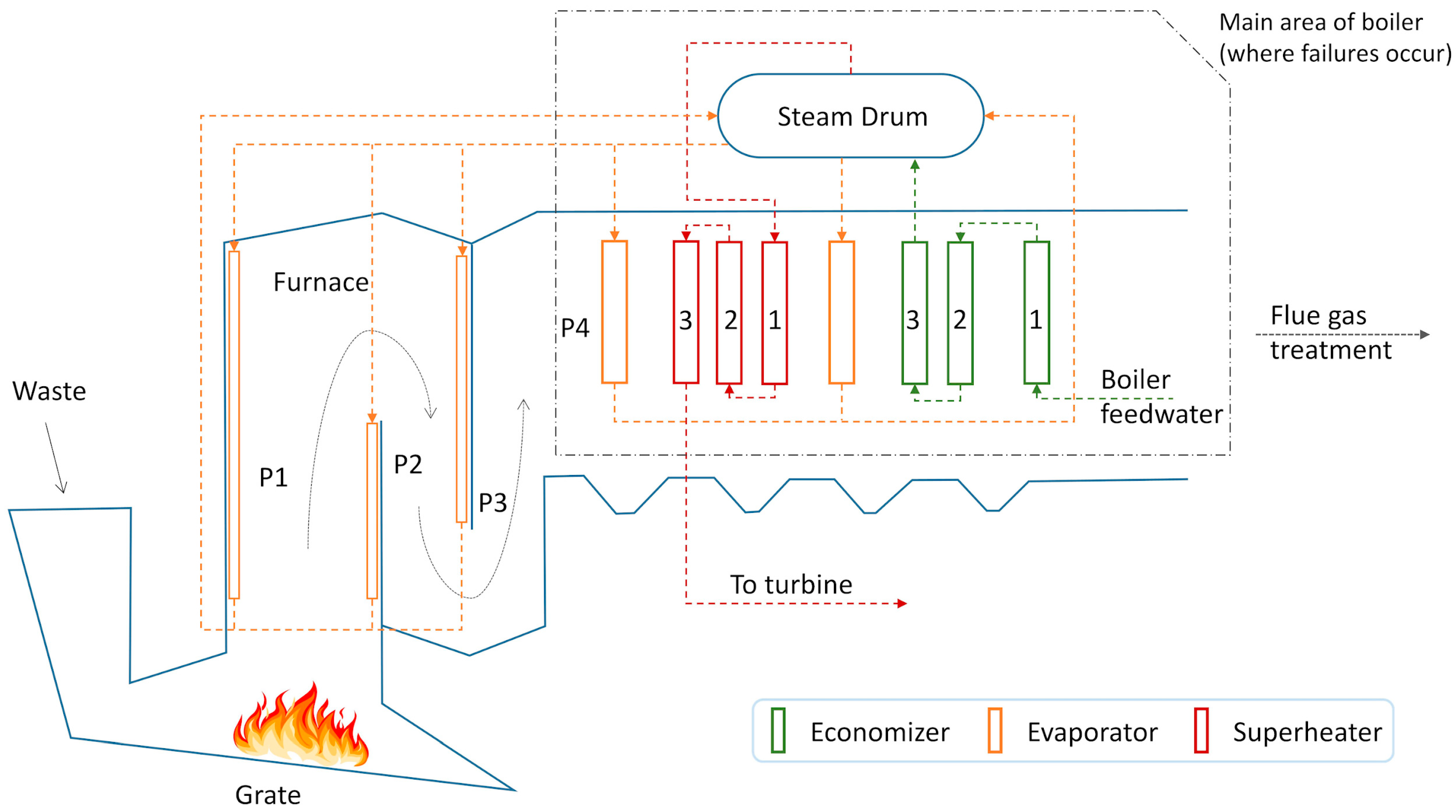
Figure 1. Boiler-related layout of Umeå WtE plant. P1, P2, P3, and P4 represent the first, second, third, and fourth flue gas passages, respectively.
Processes 12 01346 g001
Figure 2. Flowchart of the boiler failure investigation framework. Empirical engineering knowledge refers to the knowledge engineers have gained from their operating or maintenance experience, and it is grounded in physical or chemical mechanisms in the engineering context.
Processes 12 01346 g002
Figure 3. Optimal clustering result of Dataset A. Cluster 2 represents repair periods/stoppages, Cluster 1 abnormal conditions, and Cluster 0 normal conditions.
Processes 12 01346 g003
Figure 4. Histograms of Dataset A variables with significant shifts between normal and abnormal conditions. The histograms are independent of each other. For each of them, the x-axis indicates the variable value, the y-axis indicates the count/frequency of values, and the title includes the variable’s name, unit, and NPS value.
Processes 12 01346 g004
Figure 5. Optimal clustering result of Dataset B. Cluster 2 represents repair periods/stoppages, Cluster 1 abnormal conditions, and Cluster 0 normal conditions. The extremely brief appearance of Cluster 2 at the beginning reflects a transient fault in the monitoring system.
Processes 12 01346 g005
Figure 6. Histograms of Dataset B variables with significant shifts between normal and abnormal conditions. The histograms are independent of each other. For each of them, the x-axis indicates the variable value, the y-axis indicates the count/frequency of values, and the title includes the variable’s name, unit, and NPS value.
Processes 12 01346 g006
Table 1. Summary information of datasets.
Dataset IDNo. of Failures/StoppagesData ResolutionDataset Size (Row × Column)
A230 min5808 × 66
B130 min7856 × 66
Disclaimer/Publisher’s Note: The statements, opinions and data contained in all publications are solely those of the individual author(s) and contributor(s) and not of MDPI and/or the editor(s). MDPI and/or the editor(s) disclaim responsibility for any injury to people or property resulting from any ideas, methods, instructions or products referred to in the content.