Abstract
Reverse electrodialysis (RED) is one of the methods able to generate energy from the salinity gradient between sea- and river water. The technique is based on the diffusion of ions through membranes that specifically allow either cations or anions to pass through. This ion current is converted into an external electric current at electrodes via suitable redox reactions. Seawater contains mainly eight different ions and the description of transport phenomena in membranes in classical terms of isolated species is not sufficient because the different particles have different velocities—in the same direction or opposite—in the same membrane. More realistic is the Maxwell–Stefan (MS) theory that takes all interactions between the different particles in account; however, such a model is complex and validation is difficult. Therefore, a simplified system is used with solely NaCl in solution, using only 9 diffusivities in the calculation. These values are estimated from the literature and are applied to an MS model of the RED process. Using experimental data of NaCl and water transport as well as power density, these diffusivities are adapted in the MS model. Reliable values for the diffusivities were obtained for the following three interactions: H2O–Na+, H2O–Cl− and Na+–Cl−.
1. Introduction
Salinity gradient energy (SGE) can be generated from the reversible mixing of river water and seawater. It is potentially a clean and sustainable form of energy, producing brackish water and electrical energy only. The theoretical energy content of mixing 1 m3 river water with a large surplus of is 2.5 MJ or 1.7 MJ when mixed with 1 m3 [1]. The global potential of SGE is estimated to be 2.6 TW [2] which is comparable with the current world electricity consumption of about 3 TW [3] The two main membrane-based technologies that can be used to harvest this energy are reverse electrodialysis (RED) and pressure retarded osmosis (PRO) [1]. This paper is focused on RED.
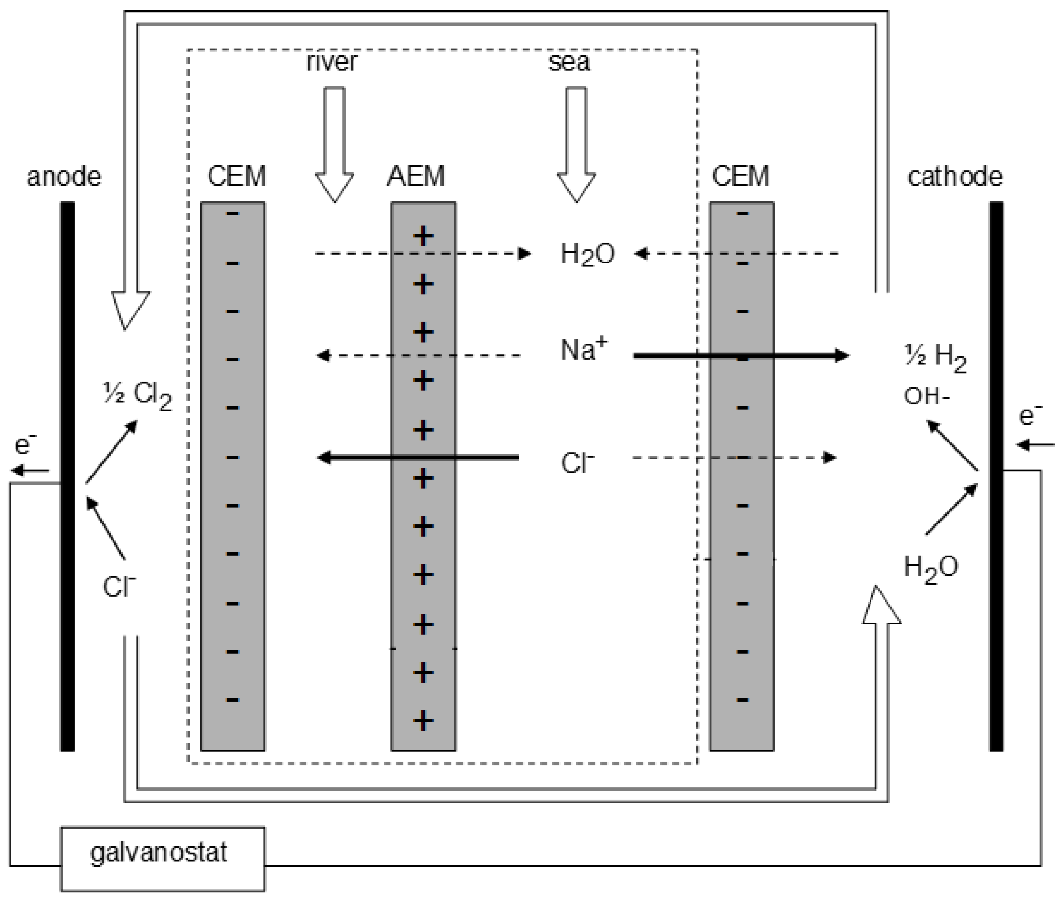
A RED stack consists of a large number of cells, each containing an anion exchange membrane (AEM), a seawater compartment, a cation exchange membrane (CEM) and a river water compartment. The stack is terminated on each side with an electrode compartment and an electrode. On one side, there is an extra ion exchange membrane (IEM), the same type as on the other side (Figure 1). The driving force in the cell is the chemical potential difference between the sea- and river water. Positive ions diffuse through the CEM from the seawater compartment to the river water compartment in one direction; the negative ions through the AEM in the other direction. The internal ionic current is converted to an external electron current on the electrodes by proper redox reactions.
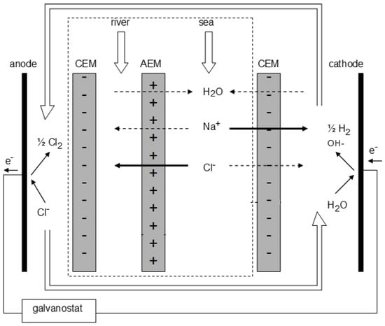
Figure 1.
A RED stack with only one cell (the part in the dashed square). Signs in the membranes represent fixed charges. Desired movements of the ions through the membranes are indicated with solid arrows and unwanted with dashed ones. The direction of the water flow is assigned to the normal osmotic flow, but may be in the opposite direction when the electro-osmotic flow dominates.
The feed consists of two solutions with different salt content: i.e., seawater with river water, Red Sea water with Dead Sea water, an industrial brine waste with seawater and so on. In this paper, we focus on the combination of seawater with river water. Table 1 shows that the main ions in seawater are Na+ and Cl− and we restrict our model to these ions.

Table 1.
Main composition of seawater with salinity 30 ‰ [4].
The feasibility of RED is described by two response parameters: power density Pd (power per m2 total active membrane) and energy efficiency Y (the generated amount of energy as part of the exergy from the inlets). In earlier experiments, we studied the effect of different parameters on these response parameters [5]. Experimental power densities are typical 1.2 W/m2. If operated under conditions of maximal power density, the energy efficiency is about 20%, increasing to more than 85% with low power density and using circulating feed waters [6]. Membrane properties are decisive for optimal operating and influence power density as well as fuel efficiency by osmosis, electro-osmosis, co-ion transport, monovalent/multivalent competition and electrical as well hydrodynamic losses.
There are two main contributors to the performance of a RED stack: the feed water supply through the spacer filled compartments (parallel to the membranes) and the ion and water transport through the membranes (perpendicular to the membranes). The first movement is described by hydrodynamics; the driving force is the pressure difference as applied by the pumps. The driving forces for ion and water transport are the chemical and electrical potentials; resistance against the particle movements is caused by friction between the different particles and between particles and immobilized charges within the membranes. This complicated process is described by the Maxwell–Stefan theory and is the subject of this paper [7,8].
A membrane has primary and secondary properties. Primary properties can be seen as the causes and include type (homogeneous or heterogeneous), ion exchange capacity, swelling degree, composition, degree of cross-linking, etc. Secondary properties are the consequences and examples are electrical resistance, counter ion permselectivity, water permeability, permselectivity for monovalent ions, density and tensile strength.
- -
- Electrical resistance: With pure NaCl solutions, the RED process is clear. A low electrical resistance is important for high power density; high permselectivity together with low osmosis is necessary for good energy efficiency. The areal resistance of common membranes as used in RED is about 2–3 Ω∙cm2 for CEMs and 1–3 Ω∙cm2 for AEMs [9].
- -
- Permselectivity for counter-ions: A second membrane parameter is the permselectivity for counter-ions. A CEM is also slightly permeable for chloride ions and an AEM for sodium ions. This transport of co-ions affects not only the generated voltage (and therewith power density), but also fuel efficiency [10]. Most common IEMs as used in RED have permselectivities of 95–100% for CEMs and 90–95% for AEMs [9].
- -
- Water permeability: Besides ions, also water can be transported through the membrane. If the RED stack is not connected to an electrical load, the ion flow through the membranes is low and the water will flow from the river water compartment to the seawater side. In fact, the water flows from high to low water concentration— a phenomenon called osmosis. However, if the stack produces power, there is an ionic flow inside the stack from the seawater to the river water compartments. Ions in aqueous solution are hydrated with a hydration number of 5.4–5.5 for Na+ and 7.1–7.3 for Cl−, depending slightly on the concentration [11]. These water molecules—in direct contact with the ion—form the inner hydration shell. The moving hydrated ions can drag even more water molecules that are situated in the so-called outer hydration shell. All attached water causes a water flow opposite the osmotic flow, a phenomenon known as electro-osmosis. Osmosis and electro-osmosis are opposite in direction and can even completely cancel each other out at a certain electrical current density [10]. In normal ED, as used for desalination, osmosis and electro-osmosis have the same direction and here too this water transport is detrimental to the energy demand of the process.
Permselectivity for monovalent ions: Most commercial membranes do not discriminate between monovalent and divalent ions. However, it was found that divalent ions in the feed waters have a negative influence on the power density of a RED stack equipped with these membranes [12,13,14,15]. The main reason that divalent ions adversely affect the operation of a RED system is their low membrane potential E. This is shown by the Donnan equation for a CEM, as follows:
where aCEM stands for the permselectivity of the CEM, R for the gas constant (8.314 J mol−1K−1), T for the temperature (K), z for the valence of the ion and F for the Faraday constant (96,485 C mol−1); activities are denoted by a, activity coefficients by γ and concentrations (mol/L) by C. Subscripts S and R are used for sea- and river water. A similar equation holds for the membrane potential over an AEM. The membrane potential is determined by the monovalent ions (z = 1) because those are in large excess and amounts to 78 mV for pure NaCl solutions of 30 g/L and 1 g/L [14]. Supposing that the membrane is part of a RED stack operating at maximum power, the voltage will drop to half, namely 39 mV. Divalent ions (z = 2) generate half of the potential of monovalent ions—assuming the same ratio of activities—and this potential is equal to that 39 mV. In that case, those ions experience no net electrical force and therefore remain at rest and do not contribute to the power output. If there are relatively more divalent ions in the river water, then there will be an uphill transport of these ions. It is clear that monovalent and divalent ions have different velocities within the membrane. A measure to mitigate the effect of divalent ions is the application of mono-selective membranes. However, these membranes have a higher resistance and ultimately yield little or no gain in power density efficiency or efficiency.
To get grip on these complex systems, Higa et al. [16,17] applied the Nernst–Planck equation to such systems. However, this method takes no account of the mutual interactions between the different particles. In the next decade, many articles were published on the multicomponent problem in ion exchange membranes using the Maxwell–Stefan (MS) theory [7,8,18,19,20]. This theory takes all interactions between ions, water molecules and fixed membrane ions into account. Movement of particles is derived from driving forces and from friction with other particles. In a RED stack—operating on pure NaCl solutions—the driving forces are the chemical and electrical potential while the process is slowed down by friction between H2O–Na+, H2O–Cl−, Na+–Cl−, Na+–~SO3−, Cl−–~NR3+, H2O–~SO3−, H2O–~NR3+, Na+–~NR3+, and Cl−–~SO3− (~NR3+ and ~SO3− are fixed charges in the AEM and CEM).The secondary properties resistance and permselectivity are dependent on these friction coefficients.
To describe the drag between particles, the MS theory uses diffusivities, inverse friction coefficients. In a simplified model of seawater as shown in Table 1, there are 8 ions; the MS approach of such a system in RED uses a total of 11 particles: the 8 mentioned for the solved ions, 1 for water and 2 for the two types of fixed charges on the membranes (AEM and CEM). All diffusivities can be written as a single 11 × 11 matrix. However, the diffusivities on the main diagonal are not interesting and the matrix is symmetrical, and therefore only 55 elements remain. Because there is no interaction between the fixed ions on the AEM and the CEM, the concerning element can be omitted, remaining 54 elements. In general—following this reasoning—with n different ions, the number of MS interactions (NMS) is as follows:
Each interaction has an associated diffusivity and with multiple ions NMS increases rapidly. Thus for pure NaCl solutions, NMS = 9 and for mixtures of NaCl and MgSO4, NMS = 40. MS-diffusivities are in most cases barely obtained. Only the system consisting of Na+, Cl− and water in membranes is well described, but it appears that the diffusivities are dependent on concentration and type of membrane. Furthermore, published data of other ions are exceptionally scare. Therefore our model and experiments are restricted to NaCl solutions only and transport phenomena through compartments and diffusion layers will not be taken in account. In this case only 2 ions remain, resulting in 9 diffusivities. The model in this paper is validated by data achieved experimentally; the transport of ions and water and electrical properties are measured and compared with the values of the model.
2. Experimental
2.1. Cell and Membranes
The RED stack that was used is described in a former paper [10]. The functional area of one membrane was 10 × 10 cm2. The stack was equipped with 25 membrane pairs of Fumasep anion and cation exchange membranes (FAD and FKD, Fumatech Bietigheim-Bissingen, Germany), thickness 0.082 mm. The stack was closed with CEMs on both ends. Polyamide woven spacers were applied between the membranes with a thickness of 200 μm (Nitex 03-300/51, Sefar, Lochem, The Netherlands).
2.2. Electrode System and Electrical Measurements
Titanium mesh electrodes coated with Ru-Ir mixed metal oxides (Magneto Special Anodes, Schiedam, The Netherlands) were applied together with an electrode rinse solution of NaCl (15 g/L). Potential measurements were performed with Ag/AgCl gel-filled reference electrodes (QM711X, ProSense, Oosterhout, The Netherlands) that were connected to the electrode compartments through Luggin capillaries.
2.3. Feed Waters
‘Seawater’ consisted of 0.5 mol/L NaCl and ‘river water’ of 0.0167 mol/L NaCl. The stack was fed with 350 mL/min of both feed waters. The temperature was controlled at 298 ± 1 K for all experiments. Salt concentrations in inlet and outlet streams were derived from measured conductivities. Flow rates were measured at the outlets of the stack. The transport of salt and water was calculated from mass balance of salt and water; the method is described in [10] and summarized in Appendix A.
3. Application of the Maxwell–Stefan Theory
The transport through a membrane is considered as a one-dimensional event in the z-direction. The MS description of species i in a mixture of n different particles in an ion exchange membrane in a RED stack, is as follows:
The left side of the equation, the gradient of the chemical potential, represents the driving force (N/mol) of species i. The right side shows the friction between species i and all other species (j = 1, …, n; j ≠ i) and, depending on the difference in average velocity (vi − vj), and the mole fraction of each other species (xj). For each combination of i with j, there is a special Maxwell–Stefan diffusivity Ðij.
The most important driving forces in the RED process are the activity gradient and the electric gradient. Used pressures in RED are low (<1 bar) with respect to the osmotic pressure of seawater (about 25 bar) and can be neglected. If the these driving forces are substituted in Equation (3) the result is:
The first term on the left side indicates the activity contribution where the mole fraction x is corrected by the activity coefficient γ. The second term is the electric part of the driving force. This equation in our model is approximated by:
The superscripts R and S indicate the boundaries in the membrane on the river water side and on the seawater side.
Maxwell–Stefan diffusivities Đ of particles in ion exchange membranes are collected from different sources as shown in Table 2. The amount of found data is rather poor; moreover, data are related to different membranes, achieved with different methods at different temperatures. The last column in the table lists the median of the different diffusivities; these are used as a starting value in the fit of the MS model.
Table 2.
Diffusivities from the literature in CEMs, AEMs and water and median values. All diffusivities are given in units of 10−10 m2/s.
4. Modelling
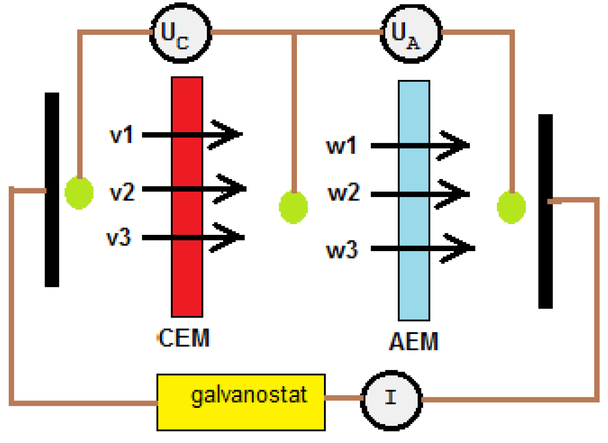
Figure 2 shows the design of the MS model. Our model is limited to transport in the membranes; mass transfer in the intermediate feed water compartments was not considered for reasons of simplicity. The variables are the velocities of the particles (v1, v2 and v3) through the CEM and (w1, w2 and w3) through the AEM. Indices 1, 2 and 3 stand for H2O, Na+ and Cl−; UC and UA are the voltages over the CEM and AEM. With the solver the 6 velocities and 2 voltages are obtained as functions of the electrical current I. The Maxwell–Stefan model consists of 5 steps which are summarized below. The program code is written in Mathcad Express Prime 9.0.0.0.0 and is available from the author.
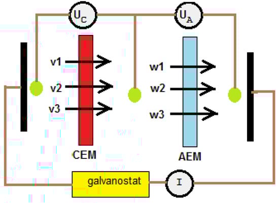
Figure 2.
Design of the MS model. In a solver box, the two membrane voltages (UC and UA) and the velocities v1, v2, v3 (for H2O, Na+ and Cl−), w1, w2 and w3 through the membranes are calculated as functions of the electrical current I.
4.1. Feed Water Concentrations
Because the experiment was performed with 7 different current densities, 7 inlet concentrations were imported for both inlet streams (S and R) and 7 for both outlet concentrations. The model used the mean value of each stream. For each of the 4 mean concentrations the activity of all ions was calculated using the extended Debye–Hückel equation. The mole fraction of each particle (ions and water) was also calculated.
4.2. Membrane Properties
The relevant membrane properties are the concentration of the fixed charges (Cn) and the total concentration of all particles (Ct); they were obtained from the reported values of the swelling degree (S), density (ρ) and the ion exchange capacity (IEC) as shown:
Here, MW is the molar mass of water (0.018 kg/mol).
4.3. Boundary Concentrations within the Membranes
The following compounds are involved in the model: H2O (1), Na+ (2), Cl− (3), for the dissolved particles and ~SO3− (4) and ~NR3+ (5) for the fixed charges in the membranes. The number between parentheses is used as an index in the notation of mole fractions, etc. Concentrations in the river and seawater compartments were taken independently of the distance to the membranes. Within the membranes there are four interfaces, indicated by the superscripts CS (CEM–Sea), CR (CEM–River), AS (AEM–Sea) and AR (AEM–River). On each interface the mole fraction of the ions in the membrane phase was calculated by applying the theory of the Donnan equilibrium [17]. For example, on the sea-CEM interface the equilibria for all charged particles are as follows:
In these expressions KCS represents the Donnan equilibrium constant for the relevant interface (CS); the power applied on K (1 and −1) is the valence of the relevant ion. To solve the system, an extra equation should be added. For reasons of electroneutrality, this is as follows:
Using Equations (8) and (9) the mole fractions x2CS and x3CS and the Donnan equilibrium constant KCS can be solved. Such systems are also solved for the other interfaces, giving the mole fractions xiCS, xiCR, xiAS, xiAR (i = 2, 3) and the equilibrium constants KCS, KCR, KAS and KAR. In this particular case, with only three unknowns, the solver function does not need to be used and the equilibrium constant K and the mole fractions of Na+ and Cl− can be solved with a quadratic equation.
4.4. The Solver Box
The solver box contains 6 equations similar to Equation (5), namely 3 for the transport of H2O, Na+ and Cl− through the CEM and 3 for the transport through the AEM. Additional equations are added for the mass balance through the membranes and for the relation between mass transport and electrical current. With these 8 equations, 8 variables are solved (v1, v2, v3, w1, w2, w3, and the voltages over the two membranes UC and UA).
4.5. Comparison of MS Model and Experiment
Power density was determined from membrane potentials and current density. The internal fluxes of ions and water were derived from the velocities and concentrations of the particles. These data were compared with the experimental values. This is discussed in the next section.
5. Results and Discussion
5.1. Adapting the Maxwell–Stefan Model
In previous experiments [10] we developed a method for measuring the transport of NaCl and H2O in a RED stack. Experimental results of a stack equipped with 25 cell pairs with Fumasep FAD and FKD membranes were compared with the MS model. Measurements were performed with seven different current densities (+20, 0, .... −100 A/m2). The comparison was based on three aspects: (i) internal water transport, (ii) internal salt transport, and (iii) power density. Together, these experiments provide a dataset consisting of 21 numbers. Using this dataset, nine diffusivities (those from Table 2 as well as one value for the internal resistance of the stack) were adapted.
The model was adapted by minimizing the sum of squared residuals SS, as follows:
where Fw stands for (electro)osmotic flux, Ts for salt transport and Pd for power density.
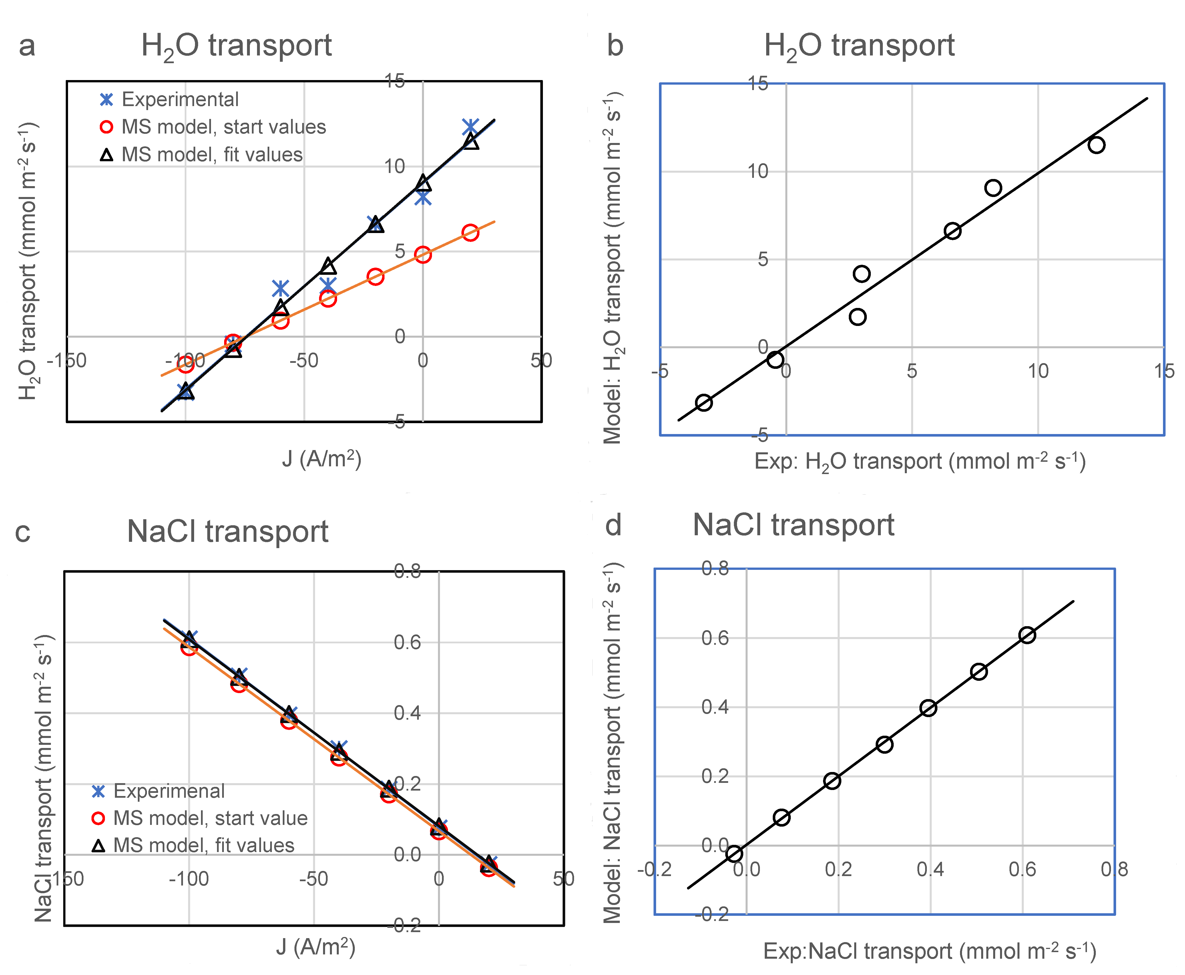
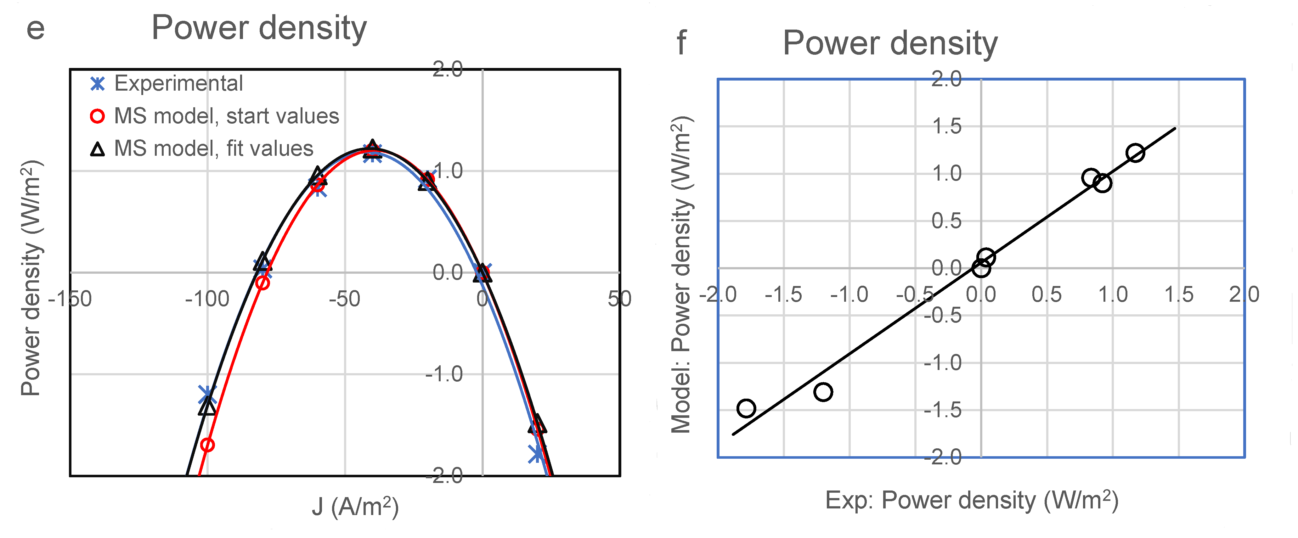
First we adjusted the internal resistance (Ri) only and used the median diffusivities from Table 2. This resulted in relatively poor agreements with experimental values as seen in Figure 3 (marked as ‘MS model, start values’). Then Ri all diffusivities were adjusted until SS reached the minimum SSmin. The same figure illustrates accordance with the experimental values (plots marked with ‘MS model, fit values’). Of interest are the coefficients of determination (R2) between the experimental and modelled data. Table 3 lists the R2 values and the equations of the regression lines from Figure 3b,d,f. The good similarity between the adapted model and the experiment is evident from the high values of R2 and the small y-intercept.
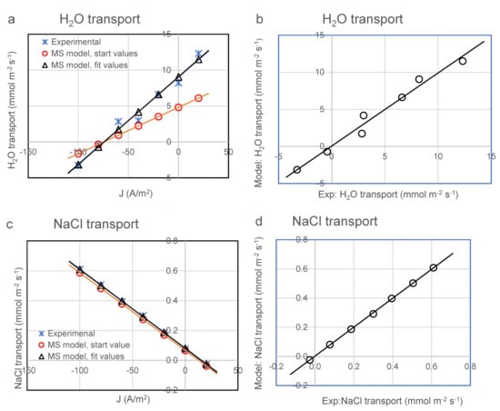
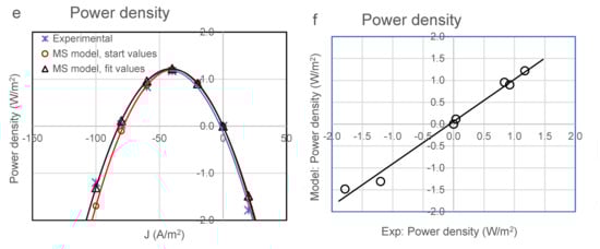
Figure 3.
(a) H2O transport from river to seawater compartment. Experimental data (*), data from the model with start values (○) and modelled data with adapted diffusivities (△) The regression lines for the experimental data and the adapted model, almost coincide. (b) H2O transport: adapted model data versus experimental data. (c) NaCl transport from sea- to river water compartment. (d) NaCl transport: adapted model data versus experimental data. (e) Power density with parabolic regression lines (partly overlapping). (f) Power density: adapted data versus experimental data.
Table 3.
Results of the fit procedure.
5.2. Diffusivities
Table 4 shows the adapted diffusivities (column ‘Adapt’). The influence of each diffusivity is tested by decreasing the value until SS-min is doubled. These values are listed in column ‘Low’. The same is done by increasing the diffusivity and listing these in column ‘High’. In column ‘Adapt’ some diffusivities appear to be very high. Because diffusivity is the inverse of the friction coefficient, friction is not measured in these cases. Other values are suspect because the range between Low and High is very large. This means that these diffusivities have little influence on the model. Therefore, only the interactions H2O–Na+, H2O–Cl− and Na+–Cl− remain as reliable. The values for these three remaining diffusivities are in the range of values in the literature for very diverse membranes as shown in Table 2.
Table 4.
MS diffusivities used in the MS model. “Start’ indicates the medial values from Table 2 which are used as a start for the adjusted procedure while “Adapt” shows the final results. Values under “Low” and “High” are obtained with double values of the minimum squared residuals.
5.3. Stack Resistance
The experimental internal resistance can be derived from the power plotted in Figure 3e. From the regression line y = 0.0007x2 − 0.0623x − 0.1273, a maximum power density is found at x = −44.5 (Jopt = 44.5 A/m2) and a maximum power density Pdmax = 1.26 W/m2. Thus the external resistance is Re = Pdmax/Jopt 2 = 0.00064 Ω m2 for a single membrane, or 0.00128 Ωm2 for a membrane pair. The external resistance is equal to the internal stack resistance if the stack is operated on maximum power delivery. The MS model used is optimized by adjusting internal resistance to 0.00149 Ω. This value is close to the experimental resistance.
5.4. Permselectivity
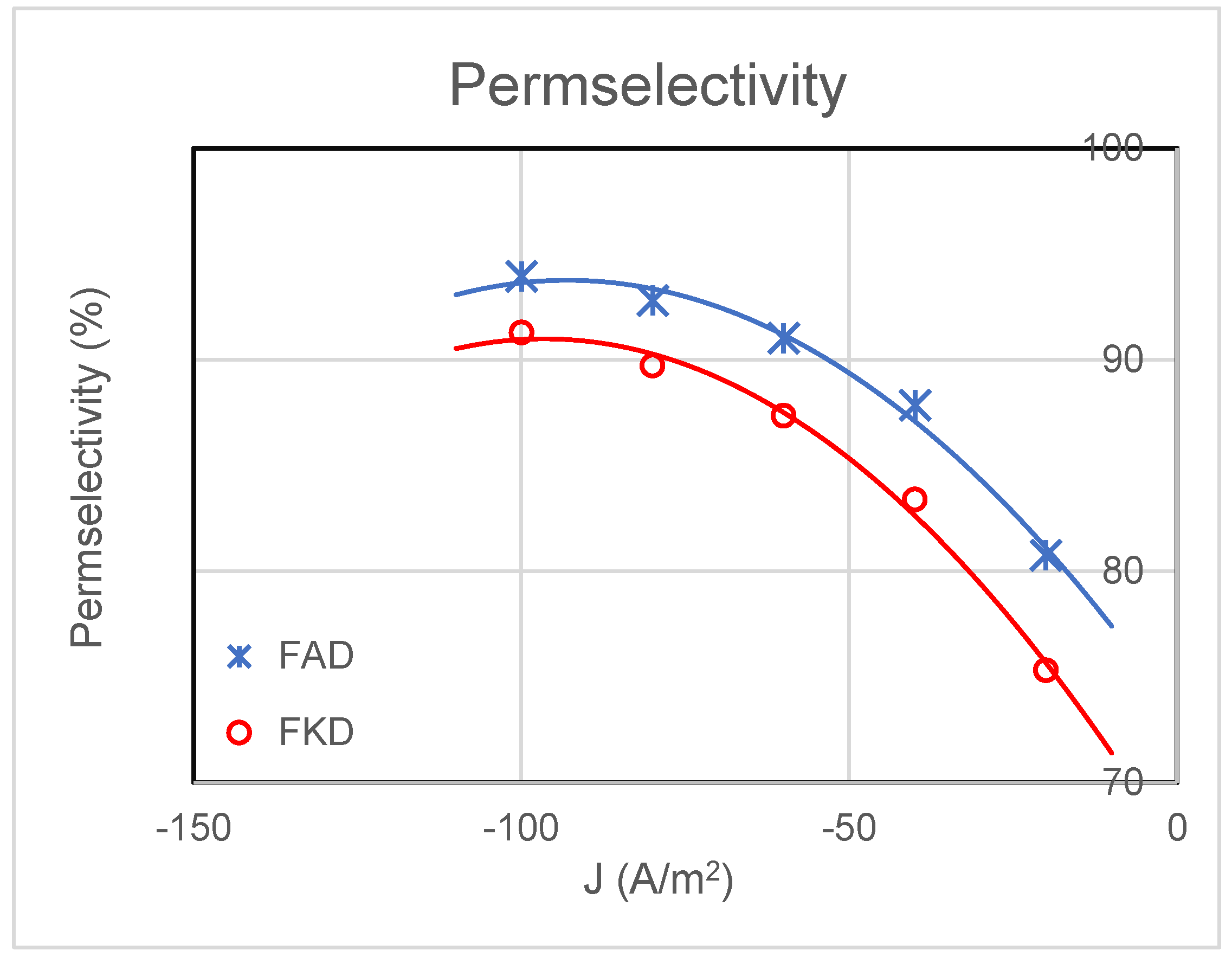
The MS model uses only swelling degree (SD), ion exchange capacity (IEC) and density (ρ) as specific input variables of the membranes. Permselectivity is not included in the model, but it follows from the calculated ion fluxes through the membranes. Figure 4 shows the permselectivity as a function of the current density. For RED, permselectivity is particularly important under conditions of maximum power delivered; for the stack used, this is at a current density of −44.5 A/m2. These values are listed in Table 5 together with values from the literature.
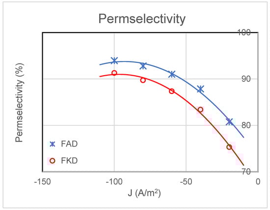
Figure 4.
Permselectivities of FAD (*) and FKD (○) membranes as function of the current density.
Table 5.
Permselectivity at J = −44.6 A/m2 is derived from the ionic fluxes in the MS model as well as from data in the literature derived from membrane potential measurements [29].
6. Conclusions and Outlook
The Maxwell–Stefan methodology provided credible values for three of the nine diffusivities. The other diffusivities have such high values that they play no role in the model. Nevertheless, after the fitting procedure, the model provided good agreements with the experimental values for (electro)osmosis, salt transport and power density which is promising for further developments in the application of the MS methodology to RED.
To achieve this, it is important to refine both experiment and model. The experiment could be improved by carrying out very accurate flow measurements, not only at the outlets, as in the experiments described in this paper and explained in Appendix A, but also at the inlet. By working with metering pumps (e.g., piston pumps) instead of peristaltic pumps, internal water transport can be measured directly. In this way, more reliable values can be achieved for the water and salt transport through membranes, parameters that are of decisive importance for the adapted procedure. Another threat is internal fluid leakage from the seawater to the river water compartment or vice versa. This may perhaps be checked with high molecular weight dyes that cannot cross the membranes themselves but can pass through the leaks in solution.
There is still a lot to be done regarding the model. At higher current intensities, internal salt transport increases and therefore the outlet concentrations change. The results described in this paper were produced using average values for inlet and outlet concentrations. As a result, the calculation of the mole fractions at the membrane interfaces is not entirely correct. A remedy could be to perform the adapted procedure for each individual amperage. That would then lead to a set of current dependent diffusivities that could be averaged afterwards.
With better coordination between experiment and model, it would be possible to include divalent ions in experiments and model. This is particularly interesting because divalent ions in a RED setup can move oppositely to monovalent ions with the same charge sign [14]. Both seawater and river water contain significant amounts of divalent ions, especially Mg2+, Ca2+ and SO42−. A better understanding of all interactions between water and free and fixed ions would be a boost for the development of RED technology as a source of renewable energy. Furthermore, this knowledge would also contribute to the development of ED, especially if this technique is used for the desalination of seawater.
Funding
This research received no external funding.
Data Availability Statement
The original contributions presented in the study are included in the article, further inquiries can be directed to the corresponding author.
Acknowledgments
This work was facilitated by REDstack BV in The Netherlands. REDstack BV aims to develop and market RED and the ED technology. The author would like to thank his colleagues from the REDstack company for fruitful discussions.
Conflicts of Interest
Author J.V. was employed by REDstack bv. The REDstack bv had no role in the design of the study; in the collection, analyses, or interpretation of data; in the writing of the manuscript, or in the decision to publish the results.
Nomenclature
| a | activity |
| C | salt content (kg∙m−3) |
| Ct | total concentration of all particles (mol∙m−3) |
| Cn | total concentration of fixed charges (mol∙m−3) |
| Đ | Maxwell–Stefan diffusivity (m2∙s−1) |
| F | Faraday constant (96,485 C∙mol−1) |
| Fw | water flux (L∙min−1) |
| I | electrical current (A) |
| IEC | ion exchange capacity (mol∙m−3) |
| J | electrical current density (A∙m−2) |
| K | Donnan equilibrium constant |
| MW | molar mass of water (0.018 kg∙mol−1) |
| NMS | number of interactions |
| n | number of particles involved |
| Pd | power density (W/m2) |
| Ri | internal resistance (Ω) |
| Re | external resistance (Ω) |
| R2 | determination coefficient |
| r | cell resistance (Ω) |
| R | gas constant (8.31432 J∙mol−1K−1) |
| S | swelling degree |
| SS | sum of squared residuals |
| Ts | salt flux |
| T | temperature (K) |
| U | electrical potential (V) |
| vi | velocity of i (m∙s−1) |
| xi | mole fraction of i |
| Y | energy efficiency |
| z | distance (m) |
| z | ionic valence |
| Greek symbols | |
| permselectivity | |
| Φ | membrane potential |
| Γ | activity coefficient |
| μii | chemical potential of i (J∙mol−1) |
| p | density (kg∙m−3) |
| Superscripts | |
| i | in |
| o | out |
| R | river |
| S | sea |
| Subscripts | |
| A | AEM |
| C | CEM |
| Abbreviations | |
| AEM | anion exchange membrane |
| CEM | cation exchange membrane |
| IEM | ion exchange membrane |
| ED | electrodialysis |
| MS | Maxwell–Stefan |
| RED | reverse electrodialysis |
| SGE | salinity gradient energy |
Appendix A. Measurement of H2O and NaCl Transport in the RED Stack
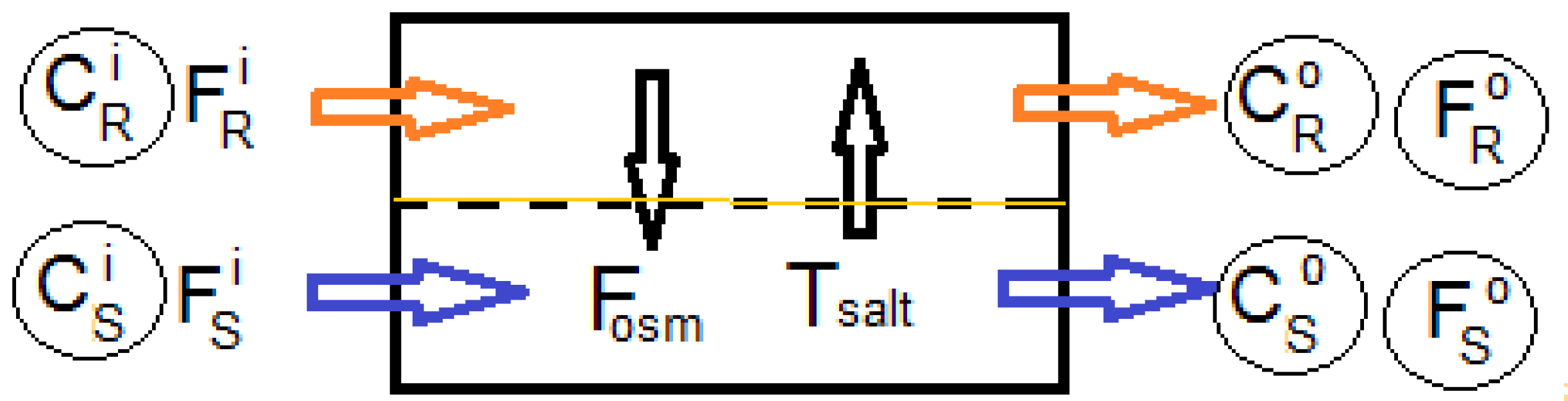
The stack was fed by peristaltic pumps which make it difficult to determine the exact flow rates. This is in contrast to the outlet flow rates, which can be determined accurately by weighting. Concentrations were determined by measuring conductivity. Figure A1 is a schematic representation of a stack, with the upper part representing all river water compartments and the lower part the seawater compartments. The dashed line represents the membranes, both the AEMs and CEMs. Variables are concentrations C (g/L), flow rates F (L/min) and mass transport numbers T (g/min). Measured values in the figure are circled and include input concentrations and and outlet concentrations and as well as measured outlet flow rates and . From these data inlet flow rates and are derived and finally internal (electro)-osmotic flow and salt transport are obtained. If electro-osmosis during operation surpasses osmotic flow, will become negative.

Figure A1.
Schematic representation of the RED stack with concentrations (C), flow rates (F) and salt transport (T). Circled values are measured and are used for calculation of the other values.
Figure A1.
Schematic representation of the RED stack with concentrations (C), flow rates (F) and salt transport (T). Circled values are measured and are used for calculation of the other values.
The mass balance applies to salt transport as follows:
Because the NaCl concentrations are not very high (<0.5 M), it is reasonable to assume that no volume contraction or expansion occurs during mixing. We therefore draw up the following volume balance:
or
Substituting (A3) in (A1):
This results in:
Now the internal streams are known as follows:
and
References
- Nijmeijer, K.; Metz, S. Chapter 5: Salinity Gradient Energy. In Sustainability Science and Engineering; Elsevier: Amsterdam, The Netherlands, 2010; Volume 2, pp. 139–295. [Google Scholar] [CrossRef]
- Wick, G.L.; Schmitt, W.R. Prospects for renewable energy from sea. Mar. Technol. Soc. J. 1977, 11, 16–21. [Google Scholar]
- International Energy Agency. World Energy Outlook 2023. Available online: https://www.iea.org/reports/world-energy-outlook-2023 (accessed on 18 January 2024).
- Lide, D.R. (Ed.) Handbook of Chemistry and Physics, 85th ed.; CRC Press: Boca Raton, FL, USA, 2004; pp. 14–16. [Google Scholar]
- Veerman, J.; Saakes, M.; Metz, S.; Harmsen, G. Reverse electrodialysis: A validated process model for design and optimization. Chem. Eng. J. 2011, 166, 256–268. [Google Scholar] [CrossRef]
- Post, J.W.; Hamelers, H.V.M.; Buisman, C.J.N. Energy Recovery from Controlled Mixing Salt and Fresh Water with a Reverse Electrodialysis System. Environ. Sci. Technol. 2008, 42, 5785–5790. [Google Scholar] [CrossRef] [PubMed]
- Wesselingh, J.A.; Krishna, R. Mass Transfer in Multicomponent Mixtures; Delft University Press: Delft, The Netherlands, 2006; ISBN 9071301583. [Google Scholar]
- Krishna, R.; Wesselingh, J. The Maxwell-Stefan approach to mass transfer. Chem. Eng. Sci. 1997, 52, 861–911. [Google Scholar] [CrossRef]
- Abidin, M.N.Z.; Nasef, M.M.; Veerman, J. Towards the development of new generation of ion exchange membranes for reverse electrodialysis: A review. Desalination 2022, 537, 115854. [Google Scholar] [CrossRef]
- Veerman, J.; de Jong, R.; Saakes, M.; Metz, S.; Harmsen, G. Reverse electrodialysis: Comparison of six commercial membrane pairs on the thermodynamic efficiency and power density. J. Membr. Sci. 2009, 343, 7–15. [Google Scholar] [CrossRef]
- Chen, H.; Ruckenstein, E. Hydrated Ions: From Individual Ions to Ion Pairs to Ion Clusters. J. Phys. Chem. B 2015, 119, 12671–12676. [Google Scholar] [CrossRef]
- Post, J.W.; Hamelers, H.V.; Buisman, C.J. Influence of multivalent ions on power production from mixing salt and fresh water with a reverse electrodialysis system. J. Membr. Sci. 2009, 330, 65–72. [Google Scholar] [CrossRef]
- Moreno, J.; Díez, V.; Saakes, M.; Nijmeijer, K. Mitigation of the effects of multivalent ion transport in reverse electrodialysis. J. Membr. Sci. 2018, 550, 155–162. [Google Scholar] [CrossRef]
- Veerman, J. Concepts and Misconceptions Concerning the Influence of Divalent Ions on the Performance of Reverse Electrodialysis Using Natural Waters. Membranes 2023, 13, 69. [Google Scholar] [CrossRef]
- Rijnaarts, T.; Huerta, E.; van Baak, W.; Nijmeijer, K. Effect of Divalent Cations on RED Performance and Cation Exchange Membrane Selection to Enhance Power Densities. Environ. Sci. Technol. 2017, 51, 13028–13035. [Google Scholar] [CrossRef] [PubMed]
- Higa, M.; Taioka, A.; Miyaska, K. Simulation of the transport of ions against their concentration gradient across charged membranes. J. Membr. Sci. 1988, 37, 251–266. [Google Scholar] [CrossRef]
- Higa, M.; Tanioka, A.; Miyasaka, K. At study of ion permeation across a charged membrane in multicomponent ion systems as a function of membrane charge density. J. Membr. Sci. 1990, 49, 145–169. [Google Scholar] [CrossRef]
- Kraaijeveld, G.; Wesselingh, J. The kinetics of film-diffusion-limited ion exchange. Chem. Eng. Sci. 1993, 48, 467–473. [Google Scholar] [CrossRef]
- Kraaijeveld, G.; Sumberova, V.; Kuindersma, S.; Wesselingh, H. Modelling electrodialysis using the Maxwell-Stefan description. Chem. Eng. J. Biochem. Eng. J. 1995, 57, 163–176. [Google Scholar] [CrossRef]
- Wesselingh, J.; Vonk, P.; Kraaijeveld, G. Exploring the Maxwell-Stefan description of ion exchange. Chem. Eng. J. Biochem. Eng. J. 1995, 57, 75–89. [Google Scholar] [CrossRef]
- Van der Stegen, J.; der Veen, A.; Weerdenburg, H.; Hogendoorn, J.; Versteeg, G. Application of the Maxwell–Stefan theory to the transport in ion-selective membranes used in the chloralkali electrolysis process. Chem. Eng. Sci. 1999, 54, 2501–2511. [Google Scholar] [CrossRef]
- Heintz, A.; Wiedemann, E.; Ziegler, J. Ion exchange diffusion in electromembranes and its description using the Maxwell-Stefan formalism. J. Membr. Sci. 1997, 137, 121–132. [Google Scholar] [CrossRef]
- Narębska, A.; Koter, S.; Kujawski, W. Irreversible thermodynamics of transport across charged membranes. Part 1—Macroscopic resistance coefficients for a system with Nafion 120 membrane. J. Membr. Sci. 1985, 25, 153–170. [Google Scholar] [CrossRef]
- PPintauro, N.; Bennion, D.N. Mass transport of electrolytes in membranes. 2 Determination of NaCl equilibrium and transport parameters for Nafion. Ind. Eng. Fundam. 1984, 23, 234–243. [Google Scholar] [CrossRef]
- Visser, R.C. Electrodialytic Recovery of Acids and Bases: Multicomponent Mass Transfer Description; Thesis Fully Internal (DIV); University of Groningen: Groningen, The Netherlands, 2001; ISBN 90-367-1359-5. [Google Scholar]
- Scattergood, E.M.; Lightfoot, E.N. Diffusional interaction in an ion-exchange membrane. Trans. Faraday Soc. 1968, 64, 1135–1146. [Google Scholar] [CrossRef]
- Schaetzel, P.; Auclair, B. Mass transfer through a weak acid ion-exchange membrane. Electrochim. Acta 1993, 38, 329–340. [Google Scholar] [CrossRef]
- Schaetzel, P.; Nguyen, Q.; Riffault, B. Statistical mechanics of diffusion in polymersConductivity and electroosmosis in ion exchange membranes. J. Membr. Sci. 2004, 240, 25–35. [Google Scholar] [CrossRef]
- Długołęcki, P.; Nymeijer, K.; Metz, S.; Wessling, M. Current status of ion exchange membranes for power generation from salinity gradients. J. Membr. Sci. 2008, 319, 214–222. [Google Scholar] [CrossRef]
Disclaimer/Publisher’s Note: The statements, opinions and data contained in all publications are solely those of the individual author(s) and contributor(s) and not of MDPI and/or the editor(s). MDPI and/or the editor(s) disclaim responsibility for any injury to people or property resulting from any ideas, methods, instructions or products referred to in the content. |
© 2024 by the author. Licensee MDPI, Basel, Switzerland. This article is an open access article distributed under the terms and conditions of the Creative Commons Attribution (CC BY) license (https://creativecommons.org/licenses/by/4.0/).