Determination of High Concentration Copper Ions Based on Ultraviolet—Visible Spectroscopy Combined with Partial Least Squares Regression Analysis

Abstract

With the rapid development of industrialization, the problem of concentration determination based on the copper production process has been widely concerned, and the accurate determination of high-concentration copper ions (Cu²⁺) is of great significance for enterprise production, resource utilization, and pollution prevention. The characteristics of different spectrophotometric methods for the determination of Cu²⁺ are discussed, and it is found that these methods are suitable for the determination of trace or low concentration of Cu²⁺ (0.5 μg/L–5 mg/L), whereas for the determination of high Cu²⁺ concentration pre-treatments such as dilution, complexation, and coloring are required. In this study, a method based on ultraviolet-visible spectroscopy (UV-Vis) combined with partial least squares regression analysis (PLS) was proposed for the determination of high copper ions (>100 mg/L), which performs rapid and accurate determination of high Cu²⁺ concentration by preprocessing and feature extraction of UV-Vis spectral data, followed by model construction with PLS analysis, which is easy to operate and applicable to a wide range of concentrations. The correlation coefficient (R²), mean relative error (MRE), and root mean square error (RMSECV) of the model prediction of Cu²⁺ concentrations were 0.99946, 0.006343, and 11.237 mg/L, respectively, indicating that the accuracy of the model prediction is very high. This study not only provides an efficient method for the precise determination of high Cu²⁺ concentration but also enables the simultaneous determination of Cu²⁺, Co²⁺, and Ni²⁺ ions, which provides a new technical means for environmental monitoring and pollution prevention.

1. Introduction

Copper is an essential material in the national economy and national defense construction. In the past decades, with the sharp increase in global copper demand, copper smelting technology has been constantly developing and progressing [1,2,3], and production capacity and output are expanding rapidly. China is the largest country in the production and consumption of refined copper, and the production of refined copper shows a rising trend from 2016 to 2022, and the production even exceeds 10 million tones after 2020 (Figure 1b). China leads the global refined copper industry in both production and consumption. In 2022, China′s refined copper production surpasses that of the second-largest producer, Chile, by over fivefold, while its consumption exceeds that of the second-largest consumer, the U.S., by more than eightfold (Figure 1a). Therefore, copper smelting is widespread throughout the world and the monitoring of copper ions is crucial.

Copper is a typical heavy metal, and there are various methods available for its determination, including spectrophotometry [4,5,6], atomic absorption spectroscopy (AAS) [7], flame atomic absorption spectroscopy (FAAS) [8,9,10,11], atomic fluorescence spectroscopy (AFS) [12], inductively coupled plasma optical emission spectroscopy (ICP-OES) [13], inductively coupled plasma mass spectrometry (ICP-MS) [14], high-performance liquid chromatography (HPLC) [15], as well as some electrochemical methods such as voltammetry [16], ion-selective electrode method [17,18,19], and polarographic analysis [20,21]. Among them, AAS, FAAS, AFS, ICP-OES, ICP-MS, and HPLC techniques have good sensitivity for the determination of trace copper, but there is a complicated pre-treatment process that introduces a major human error for the determination of high concentration samples [22]. Spectrophotometry, on the other hand, is a method that involves determining the absorbance of a substance at specific wavelengths or within a certain wavelength range to analyze the substance qualitatively and quantitatively. It has the advantages of high sensitivity, easy operation, and rapidity and is the most commonly used experimental method in biochemistry experiments [23,24].

Ultraviolet-visible spectrophotometry is a typical method within spectrophotometry that is based on the mechanism of the varying absorption of light by a substance at different wavelengths [25,26,27]. The sodium diethydlthiocabamate spectrophotometric method and the 2,9-Dimethy-1,10-phenanthroline spectrophotometric method are the two Environmental Protection Standards of the People’s Republic of China for the determination of copper in water [28,29]. Wen et al. [4] determined copper in water and food samples by dispersive liquid-liquid microextraction coupled with UV-visible spectrophotometry, with a detection limit of 0.5 μg/L. Pourbasheer et al. [5] designed a novel optical sensor for the determination of trace copper in real samples by UV/Vis spectrophotometry, with a detection range of 0.0448–6.4 mg/L for Cu(II) and a detection limit of 0.016 mg/L. Shpigun et al. [23] used a flow-injection spectrophotometric method for the simultaneous determination of Cu(II) and Zn(II). The linear range of Cu(II) detection was in the range of 0.2–3.5 mg/L. Garcia Rodriguez et al. [30] achieved the simultaneous determination of Fe(II), Co(II), Ni(II), Cu(II) by UV/Vis spectrophotometry and the linear range of Cu(II) detection was in the range of 0.2–1.5 mg/L. Zhou et al. [31] proposed a spectrophotometric method combining Kalman filtering and the derivative method, which can achieve the simultaneous determination of Co, Ni, and Cu in zinc sulphate solution, and the detection range of Cu was 0.5–5 mg/L. Zhou et al. [32] also proposed a spectrophotometric method combining continuous wavelet transform and over-zero technique, which can achieve the simultaneous detection of Co and Cu, and the detection range of Cu is also 0.5–5 mg/L. Although the above copper determination based on UV-visible spectrophotometry is feasible, it is only applicable to the determination of low-concentration copper ions (range 0.5 μg/L–5 mg/L), and the monitoring of high-concentration copper ions still requires pre-treatment such as dilution, complexation, and coloring, so the application in the actual industry is still restricted. In view of this problem, this study investigates the theoretical method for monitoring high concentrations of copper ions (>100 mg/L) and establishes a monitoring method applicable to high concentrations of copper ions in industry.

One commonly utilized modeling approach is linear modeling, with multiple linear regression being frequently employed to investigate the relationships between variables. This regression analysis method requires a relatively high sample capacity and is unable to eliminate multicollinearity among variables, thus leading to potential issues of parameter distortion in the model [33,34,35]. Principal Component Analysis (PCA) is a statistical method that involves the orthogonal transformation of a set of potentially correlated variables into a set of linearly uncorrelated variables [36]. These transformed variables, known as principal components, represent a dimensionality reduction technique [37,38]. Canonical correlation analysis is a statistical method used to study the relationship between two sets of variables. The fundamental principle of this analysis is to extract two representative composite variables, U₁ and V₁, from each set of variables, and then utilize the correlation between these two composite variables to reflect the overall correlation between the two sets of indicators [39,40]. The Partial Least Squares (PLS) regression analysis method is a typical full-spectrum, multivariate calibration method that combines multiple linear regression, principal component analysis, and canonical correlation analysis [41,42]. This method first extracts the principal components of the spectrum and establishes a multivariate statistical regression model between the principal components and sample concentrations [43,44]. PLS simultaneously decomposes the independent variable concentration matrix C and the dependent variable spectrum matrix A into principal components, extracting composite variables that have the strongest explanatory power for the dependent variable. This approach maximizes the correlation between the spectral principal components and concentrations, thereby overcoming the negative effects of multicollinearity and further enhancing the reliability of the model.

2. Materials and Methods

2.1. Materials and Sample Preparation

To understand the characteristics of copper smelting wastewater, copper smelting wastewater from a copper smelting plant in Guangxi, China, was selected to determine the main components and content, and the results are shown in

Table 1. Species and concentration ranges in typical copper smelting wastewater.

Component	Content	Units
Cu	200–3500	mg/L
Ni	1000–8000	mg/L
Co	50–200	mg/L
Fe	500–2000	mg/L
Bi	0–200	mg/L
As	500–20,000	mg/L
H2SO4	35–240	g/L

below. As can be seen from the table, copper smelting wastewater mainly contains H₂SO₄, As, Ni, Cu, Fe, Co, Bi, and the concentration of each substance fluctuates within a certain range. Particularly, the content of H₂SO₄ in the wastewater is up to 35–240 g/L. Therefore, sulfate was used as the raw material for sample preparation in this study. Ultrapure water (18.2 MΩ) from the Milli-Q water purification unit was used for dissolving and diluting in the sample preparation process. Ni²⁺ and Co²⁺ solutions of different concentrations were prepared with analytically pure grades of NiSO₄·6H₂O (98.5%) and CoSO₄·7H₂O (99.5%), respectively. Analytically pure CuSO₄·5H₂O (99%) was applied as the raw material, and various concentrations of Cu²⁺ solutions were prepared with a gradient increase starting from 100 mg/L, resulting in solutions within the concentration range of 100 to 7700 mg/L.

2.2. The Collection of UV-Visible Spectra

Since there is background absorption interference during the spectral measurement, the background interference was deducted by using ultrapure water as a blank. Then, the UV-visible spectra of the Cu²⁺ solutions were measured with the reference of ultrapure water in four different thicknesses of cuvettes, namely, 20 mm, 30 mm, 50 mm, and 100 mm, respectively. The UV-visible spectra of Ni²⁺ and Co²⁺ solutions were determined in a 50 mm cuvette with ultrapure water as a reference. Featuring a hybrid C-T double monobloc optical system with specially coated high-reflective optics (grating) and a high-performance deuterium lamp as the UV source, the T10 CS UV-visible spectrophotometer from Beijing PuXi General Instrument Co., Ltd., Beijing, China, is equipped with the UV-Win computer software for controlling the spectrometer and for data collection.

2.3. Data Processing

UV-vis spectra data plotting and processing by first and second order derivatives was conducted by origin 2024; and PLS fitting and validation were run by SPSS 26.

3. Results and Discussion

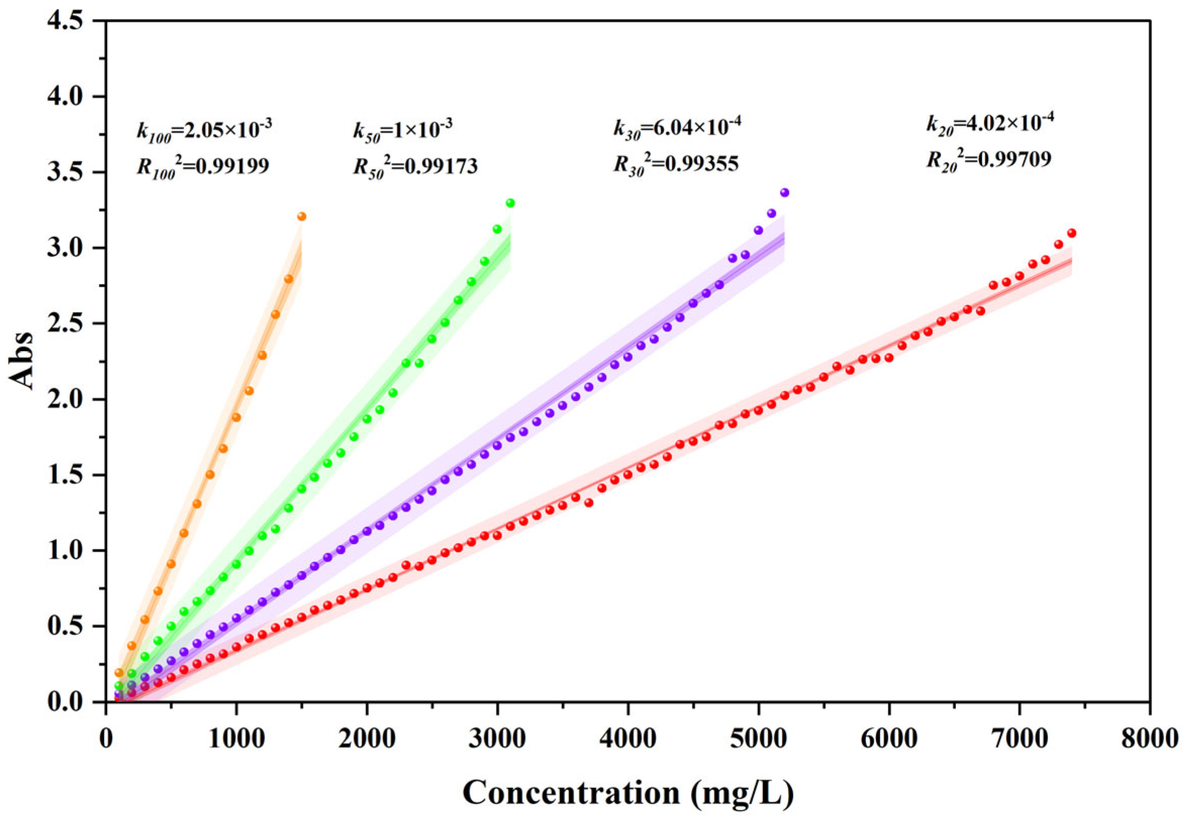
3.1. Determination of Optical Parameters

The determination of copper in the national environmental protection standards of the People′s Republic of China is carried out using the sodium diethyldithiocarbamate and the 2,9-dimethyl-1,10-phenanthroline spectrophotometric method. Both methods require the sample to undergo dilution, acidification, complexation, and color development. The detection ranges of these two methods are 0.04–6 mg/L and 0.08–3.2 mg/L, respectively. However, these methods are associated with issues such as lengthy pretreatment times, complexity of operation, potential for secondary pollution, and a limited detection range [45]. And for high-concentration samples, multiple dilutions are necessary for analysis, introducing uncertainty errors due to manual handling. To address these challenges, this study adopts a fundamental approach known as the UV-visible spectrophotometric direct measurement method. This method involves directly measuring the UV-visible spectrum of high-concentration copper samples without the need for complex pretreatments such as dilution, acidification, complexation, and color development. Samples of varying concentration gradients are scanned using a T10 CS UV-visible spectrophotometer to obtain a series of spectral curves. By analyzing these spectral curves, the optimal optical parameters for monitoring are determined. The fundamental principle followed by UV-visible spectrophotometry is the Lambert-Beer Law [46,47], expressed as Equation (9).

A = lg(1/T) = −lg(I₀/I) = ε(λ)bc

(1)

Here, A represents absorbance; T is the transmittance ratio; I₀ is the incident intensity; I is the transmitted intensity; ε is the molar absorbance coefficient, which is dependent on the properties of the substance and the incident light wavelength λ; b is the thickness of the absorbing layer; and c is the concentration of the substance (mol/L).

The UV-visible spectra of the solutions were measured in four different thicknesses of cuvettes, namely 20 mm, 30 mm, 50 mm, and 100 mm, as depicted in Figure 2a–d. It is evident from the figures that the maximum absorption peak of Cu²⁺ is located at 810 nm, and the maximum absorbance significantly increases with the rise in Cu²⁺ solution concentration. When the Cu²⁺ solution concentration is fixed, the UV-visible spectra are illustrated in Figure 2e,f. It is observed from the figures that as the thickness of the cuvette (i.e., the absorption layer thickness) increases, the maximum absorbance of Cu²⁺ gradually rises. Upon reaching a Cu²⁺ solution concentration of 5000 mg/L, a path length of 50 mm exceeds the measurement range of the UV-visible spectrophotometer. However, a path length less than 50 mm may result in low sensitivity for the concentration determination of Cu²⁺ at the hundred mg/L level.

The C-A curves of Cu²⁺ solution at different optical path lengths are shown in Figure 3, and it can be seen that the R² of the C-A fitted curves under four different optical paths are all greater than 0.99, which indicates that the fitted curves can well respond to the relationship of absorbance with Cu²⁺ concentration. ΔA/ΔC can be used to express the sensitivity of concentration detection [48], which can be approximated by the slope k on the C-A curve, and it can be seen from Figure 3 that the sensitivity is k₁₀₀ > k₅₀ > k₃₀ > k₂₀. The upper limits of concentration reached by the fitted curves at path lengths of 20 mm, 30 mm, 50 mm, and 100 mm are 7700 mg/L, 5400 mg/L, 3200 mg/L, 1500 mg/L, 1500 mg/L, and 3200 mg/L, respectively. Meanwhile, considering the actual concentrations of Cu²⁺ in acidic wastewater from the copper smelting industry, which can reach levels above a thousand mg/L but generally not exceeding 5000 mg/L (Table 1), an excessively large path length could lead to concentrations of Cu²⁺ in the solution surpassing the detection limit of the spectrophotometer. So combining the concentration range of Cu²⁺ in copper smelting wastewater and the scale of sensitivity, the optimal absorption wavelength is determined to be 810 nm, with a maximum path length of 50 mm.

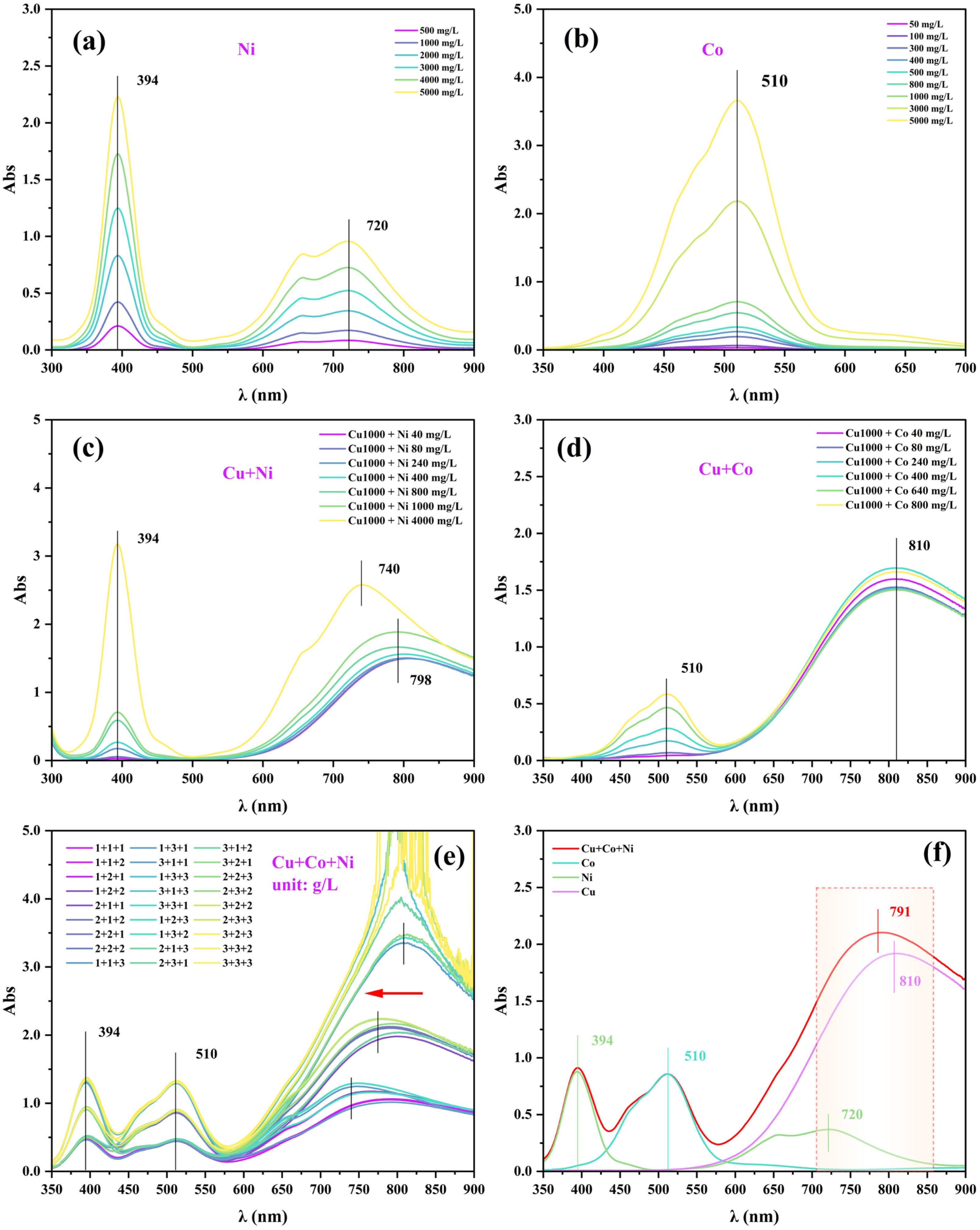
3.2. Influence of Interfering Factors

Ni²⁺ and Co²⁺ ions are coexisting metal ions in copper smelting wastewater. Nickel sulfate (NiSO₄) and cobalt sulfate (CoSO₄) dissolve in aqueous solution to exhibit green and red colors, respectively, while copper sulfate (CuSO₄) dissolution results in a blue color. Therefore, the mixed color changes in the presence of Ni²⁺ and Co²⁺ ions in the solution can interfere with the detection of Cu²⁺ ion concentration using UV-visible spectrophotometry [49]. To assess the extent of interference of Ni²⁺ and Co²⁺ ions on the detection of Cu²⁺ ions, individual UV-visible spectroscopic analyses were conducted for Ni²⁺ and Co²⁺ ions. Additionally, different concentrations of Ni²⁺ and Co²⁺ ions were separately added to solutions with Cu²⁺ ions for UV-visible spectroscopic analysis. The results are depicted in Figure 4. The UV-visible spectra revealed that Ni²⁺ ions exhibit two distinct maximum absorption peaks at 394 nm and 720 nm (Figure 4a), with the maximum absorbance values showing systematic changes with concentration. The maximum absorption wavelength for Co²⁺ ions is 510 nm, and its maximum absorbance values increase systematically with concentration (Figure 4b). When Cu²⁺ ions are mixed with Ni²⁺ ions, significant changes in the absorption peak of Cu²⁺ ions at 810 nm are observed. The maximum absorption peak position of Cu²⁺ ions in the mixed solution undergoes noticeable changes (Figure 4c), and the mixed solution also affects the absorption peak of Ni²⁺ ions at 720 nm. When Cu²⁺ ions are mixed with Co²⁺ ions, it is observed from Figure 4d that the maximum absorption peak positions of Cu²⁺ ions and Co²⁺ ions do not change due to their mixture. However, the maximum absorption intensity values of Cu²⁺ ions at the same concentration will irregularly vary with changes in the concentration of Co²⁺ ions. Since the maximum absorption peak position of Cu²⁺ ions is located at 810 nm, which is close to the maximum absorption peak position of Ni²⁺ ions at 720 nm, the overlapping effect of their absorption wavelengths in the range of 720 to 810 nm will impact the absorption peaks of both ions. Figure 4e presents the absorption spectra of mixed solutions of Cu²⁺, Co²⁺, and Ni²⁺ with different concentration combinations, and the positions of the maximum absorption peaks at 394 nm for Ni²⁺ and 510 nm for Co²⁺ do not vary, whereas the positions of the maximum absorption peaks at 720 nm for Ni²⁺ and 810 nm for Cu²⁺ near the NIR region are significantly shifted with the mixing of the three and the change in their concentrations. Thus, the interfering ions affect the absorption spectrum of Cu²⁺. In Figure 4f, the UV-visible absorption spectral curves of Co²⁺, Ni²⁺, and Cu²⁺ are cyan, green, and violet, respectively, and the spectral curve of the mixed solution of the three is red, and the mixed solution obviously affects the maximal absorption wavelength of Cu²⁺ at 810 nm, which is consistent with the results in Figure 4e.

The original spectrum of the mixed solution in UV-visible spectroscopy may be influenced by factors such as background noise and baseline drift [50]. To eliminate irrelevant interference from the surrounding environment during the experimental process, mixed solution original spectra with maximum absorbance values below 3.0 were selected for first-order and second-order derivative processing [51,52]. The original spectra, as well as the spectra after first-order and second-order derivative processing, are shown in Figure 5. A comparison reveals that at the maximum absorption wavelength positions of Ni²⁺ and Co²⁺ at 394 nm and 510 nm, background noise from the environment and instrumentation does not have a significant impact. However, at the wavelength corresponding to the maximum absorption peak of Cu²⁺, the spectrum is irregularly affected by background noise and the Ni²⁺ absorption peak.

3.3. Establishment of Monitoring Model

Assuming there are n standard mixed concentrations composed of m components, if the absorbance of the solution is measured at l wavelength points, the absorbance matrix A(n,l) and concentration matrix C(n,m) can be obtained. The specific steps of partial least squares regression are as follows:

i.

Extract the first components u₁ and v₁ from the absorbance matrix and concentration matrix.

The variable u₁ is a linear combination of the independent variable set A = [a₁, …,a_l]^T, expressed as u₁ = α₁₁a₁ +…+ α_1la_l = ρ^(1)TA.

Similarly, the variable v₁ is a linear combination of the dependent variable set C = [c₁, …,c_m]^T given by v₁ = β₁₁c₁ +…+β_1mc_m = γ^(1)TC.

The objectives for u₁ and v₁ are twofold: (1) to extract as much variability from their respective variable sets as possible, and (2) to maximize the correlation between u₁ and v₁.

By utilizing the standardized observed data matrices T and U of the two variable sets, the score vectors for the first pair of components can be computed and denoted as ${\widehat{u}}_1$ and ${\widehat{v}}_1$.

$${\widehat{u}}_1=T{\rho }^{\left(1\right)}=\left[\begin{array}{ccc}{t}_{11}& \cdots & t_{1l}\\ ⋮& & ⋮\\ t_{n1}& \cdots & t_{nl}\end{array}\right]\left[\begin{array}{c}{\alpha }_{11}\\ ⋮\\ {\alpha }_{1l}\end{array}\right]$$

(2)

$${\widehat{v}}_1=U{\gamma }^{\left(1\right)}=\left[\begin{array}{ccc}{u}_{11}& \cdots & u_{1m}\\ ⋮& & ⋮\\ u_{n1}& \cdots & u_{nm}\end{array}\right]\left[\begin{array}{c}{\beta }_{11}\\ ⋮\\ {\beta }_{1p}\end{array}\right]$$

(3)

The covariance $\mathrm{Cov}(u_1,v_1)$ between the first pair of components $u_1$ and $v_1$ can be calculated using the inner product of the score vectors ${\widehat{u}}_1$ and ${\widehat{v}}_1$ of the first pair of components. Therefore, the aforementioned requirements can be transformed into a mathematical problem of optimizing conditions.$\mathit{max}<{\widehat{u}}_1\cdot {\widehat{v}}_1>=<A{\rho }^{\left(1\right)}\cdot B{\gamma }^{\left(1\right)}>={\rho }^{\left(1\right)T}{T}^{T}U{\gamma }^{\left(1\right)}$.

$$\mathrm{s}.\mathrm{t}.\hspace{0.33em}\left\{\begin{array}{c}{\rho }^{\left(1\right)T}{\rho }^{\left(1\right)}={‖{\rho }^{\left(1\right)}‖}^2=1,\\ {\gamma }^{\left(1\right)T}{\gamma }^{\left(1\right)}={‖{\gamma }^{\left(1\right)}‖}^2=1.\end{array}\right.$$

(4)

utilizing the Lagrange multiplier method, the problem is transformed into finding the unit vectors ${\rho }^{\left(1\right)}$ and ${\gamma }^{\left(1\right)}$ that maximize ${\theta }_1={\rho }^{\left(1\right)T}{T}^{T}U{\gamma }^{\left(1\right)}$. The solution to the problem only requires computing the eigenvalues and eigenvectors of the $m\times m$ matrix $M=T^{T}U{U}^{T}T$, where the largest eigenvalue of M is ${\theta }_1^2$. The corresponding unit eigenvector is the desired solution ${\rho }^{\left(1\right)}$, while ${\gamma }^{\left(1\right)}$ can be calculated from ${\rho }^{\left(1\right)},$ as follows:

$${\gamma }^{\left(1\right)}=\frac{1}{{\theta }_1}{U}^{T}T{\rho }^{\left(1\right)}$$

(5)

ii.

Establish regressions of $c_1,\cdots ,c_m$ on $u_1$ and $a_1,\cdots ,a_l$ on $u_1$. Assume the regression model is as follows:

$$\left\{\begin{array}{c}T={\widehat{u}}_1{\sigma }^{\left(1\right)T}+T_1,\\ U={\widehat{u}}_1{\tau }^{\left(1\right)T}+U_1,\end{array}\right.$$

(6)

where ${\sigma }^{\left(1\right)}=[{\sigma }_{11},\cdots ,{\sigma }_{1l}{]}^T$ and ${\tau }^{\left(1\right)}=[{\tau }_{11},\cdots ,{\tau }_{1m}{]}^T$ are parameter vectors in the one-to-many regression model, $T_1$ and $U_1$ are residual matrices.

The least squares estimate of the regression coefficient vectors ${\sigma }^{\left(1\right)}$ and ${\tau }^{\left(1\right)}$ are as follows:

$$\left\{\begin{array}{c}{\sigma }^{\left(1\right)}=\frac{A^T{\widehat{u}}_1}{{‖{\widehat{u}}_1‖}^2,}\\ {\tau }^{\left(1\right)}=\frac{B^T{\widehat{u}}_1}{{‖{\widehat{u}}_1‖}^2,}\end{array}\right.$$

(7)

These vectors ${\sigma }^{\left(1\right)}$ and ${\tau }^{\left(1\right)}$ are referred to as the model effect loadings.

iii.

Substitute the residual matrices $T_1$ and $U_1$ for $T$ and $U$, and repeat the aforementioned steps.

Let $\widehat{T}={\widehat{u}}_1{\sigma }^{\left(1\right)T}$ and $\widehat{U}={\widehat{u}}_1{\tau }^{\left(1\right)T}$, then the residual matrices $T_1=T-\widehat{T}$ and $U_1=U-\widehat{U}$. If the absolute value of the elements in the residual matrix $U_1$ is approximately 0, the accuracy of the regression equation built with the first component considered to be sufficient and the extraction of components can be discontinued. Otherwise, repeat the above steps with residual matrix $T_1$ and $U_1$ instead of $T$ and $U$, i.e., to get ${\rho }^{\left(2\right)}=[{\alpha }_{21},\cdots ,{\alpha }_{2l}{]}^T$ and ${\gamma }^{\left(2\right)}=[{\beta }_{21},\cdots ,{\beta }_{2m}{]}^T$. Whereas ${\widehat{u}}_2=T_1{\rho }^{\left(2\right)}$ and ${\widehat{v}}_2=U_1{\gamma }^{\left(2\right)}$ are the score vectors for the second pair of components, the ${\sigma }^{\left(2\right)}=\frac{A_1^T{\widehat{u}}_2}{{‖{\widehat{u}}_2‖}^2}$ and ${\tau }^{\left(2\right)}=\frac{B_1^T{\widehat{u}}_2}{{‖{\widehat{u}}_2‖}^2}$ are the loadings of the second pair of components of $A,C$, respectively. At this point there are:

$$\left\{\begin{array}{c}T={\widehat{u}}_1{\sigma }^{\left(1\right)T}+{\widehat{u}}_2{\sigma }^{\left(2\right)T}+T_2,\\ U={\widehat{u}}_1{\tau }^{\left(1\right)T}+{\widehat{u}}_2{\tau }^{\left(2\right)T}+U_2.\end{array}\right.$$

(8)

iv.

Given the rank of the $n\times l$ data matrix $T$ is $r\le \mathit{min}(n-1,l)$, there exist $r$ components $u_1,u_2,\cdots ,u_r$ that make

$$\left\{\begin{array}{c}T={\widehat{u}}_1{\sigma }^{\left(1\right)T}+\cdots +{\widehat{u}}_r{\sigma }^{\left(r\right)T}+T_r,\\ U={\widehat{u}}_1{\tau }^{\left(1\right)T}+\cdots +{\widehat{u}}_r{\tau }^{\left(r\right)T}+U_r.\end{array}\right.$$

(9)

Substitution $u_i={\alpha }_{i1}{a}_1+\cdots +{\alpha }_{il}{a}_l$($i=\mathrm{1,2},\cdots ,l$) into $C=u_1{\tau }^{\left(1\right)}+\cdots +u_r{\tau }^{\left(r\right)}$, the partial least squares regression equation for the $m$ dependent variables is obtained as follows:

$$c_j=k_{j1}{a}_1+\cdots +k_{jl}{a}_l,\hspace{0.33em}\hspace{0.33em}j=\mathrm{1,2},\cdots ,m.$$

(10)

v.

Cross validation test.

In general, partial least squares does not require the selection of r components $u_1,u_2,\cdots ,u_r$ to build the regression equation, but rather, like principal component analysis, only the first s components ($s\le r$) are selected to obtain a regression model with better predictive ability. For the number of components $l$ to be extracted for modeling, this can be determined by a cross validity test.

The $t$-th observed data ($t=\mathrm{1,2},\cdots ,n$) are rounded off each time, and the remaining $n-1$ observed data are modeled by partial least squares regression with the fitted regression equation considering the extraction of $h(h\le r$) components, and then the $t$-th observed data of the set of rounded off independent variables is substituted into the fitted regression equation to obtain the predicted value of $c_j(j=\mathrm{1,2},\cdots ,m)$ at the $t$-th observed data ${\widehat{b}}_{\left(t\right)j}(h)$. Repeating the above validation for $t=1,$ $2,\cdots ,n$, the sum of squared prediction errors for the j-th dependent variable $c_j(j=\mathrm{1,2},\cdots ,m)$ at the time of extraction of $h$ components is derived:

$${\mathrm{PRESS}}_j(h)={\sum }_{t=1}^n(b_{tj}-{\widehat{b}}_{(t)j}(h){)}^2,\hspace{0.33em}\hspace{0.33em}j=\mathrm{1,2},\cdots ,m,$$

(11)

The sum of squared prediction errors for $C=[c_1,\cdots ,c_m{]}^T$ is:

$$\mathrm{PRESS}(h)={\sum }_{t=1}^m{\mathrm{PRESS}}_j(h)$$

(12)

In addition, the regression equation with $h$ components is again fitted using all sample points. At this point, remembering that the predicted value of the $t$-th sample point is ${\widehat{b}}_{tj}(h)$, then the sum of squares of errors of $c_j$ can be defined as:

$$\mathrm{S}{\mathrm{S}}_j(h)={\sum }_{t=1}^n[b_{tj}-{\widehat{b}}_{tj}(h){]}^2$$

(13)

Define the sum of squares of errors of $C$ as:

$$\mathrm{SS}(h)={\sum }_{j=1}^m\mathrm{S}{\mathrm{S}}_j(h)$$

(14)

When $\mathrm{PRESS}(h)$ reaches the minimum value, the corresponding $h$ is the desired number of components $s$. Normally, there is always $\mathrm{PRESS}(h)$ > $\mathrm{SS}(h)$ and $\mathrm{SS}(h)$ < $\mathrm{SS}(h-1)$. Therefore, when extracting the composition, it is always desirable the $\frac{\mathrm{PRESS}(h)}{\mathrm{SS}(h-1)}$ ratio as small as possible. Generally, a limiting value of 0.05 can be set, i.e., when $\frac{\mathrm{PRESS}(h)}{\mathrm{SS}(h-1)}\le (1-0.05{)}^2=0.95^2$, increasing the component $u_h$ is favorable to the model accuracy. Or, conversely, when $\frac{\mathrm{PRESS}(h)}{\mathrm{SS}(h-1)}>0.95^2$, it is assumed that the addition of the new component $u_h$ has no significant improvement in reducing the prediction error of the equation. For this reason, cross validity is defined as:

$$Q_h^2=1-\frac{\mathrm{PRESS}(h)}{\mathrm{SS}(h-1)}$$

(15)

In this way, the cross-validity test is performed at the end of each computational step of the modeling, if there is $Q_h^2<1-0.95^2=0.0975$ at step $h$, the model meets the accuracy requirement and the extraction of the components can be stopped. If $Q_h^2\ge 0.0975$, it means that the marginal contribution of the $u_h$ component extracted in step $h$ is significant, and the computation should be continued at step $h+1$.

R², mean relative error (MRE), and root mean square error (RMSECV) are usually used in cross-finite validation to evaluate the prediction effect of the model [53,54]:

$$R^2=1-\frac{\sum _{i=1}^n{\left(c_i-{\widehat{c}}_i\right)}^2}{\sum _{i=1}^n{\left(c-{\overline{c}}_i\right)}^2}$$

(16)

$$MRE=\frac{1}{n}{\sum }_{i=1}^n\left|\frac{c_i-{\widehat{c}}_i}{c_i}\right|$$

(17)

$$RMSECV=\sqrt{\frac{\sum _{i=1}^n{\left(c_i-{\widehat{c}}_i\right)}^2}{n}}$$

(18)

where n is the number of samples, $c_i$ and ${\widehat{c}}_i$ are the measured and predicted values of the i-th sample, respectively, and ${\overline{c}}_i$ is the average of the true values of all the samples in the training or prediction set. R² is the ratio of the regression sum of squares to the total sum of squares, and the closer the value is to 1, the better the regression model works. The root mean square error RMSECV is a measure of the deviation of the predicted value from the true value, and the smaller its value, the better the model prediction and the higher the model accuracy.

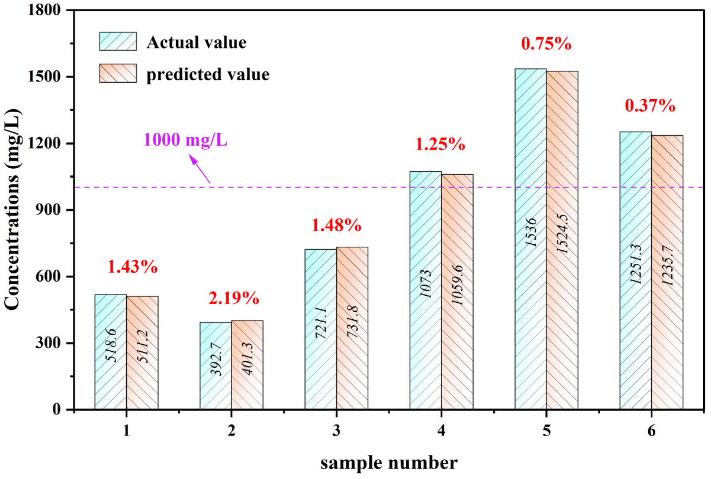
3.4. Validation of the Model

In this study, the UV-visible spectra of mixed solutions of Cu²⁺, Co²⁺, and Ni²⁺ were modeled using partial least squares regression analysis. The 18 sets of mixture spectral data with maximum absorbance values below 3.0 were selected as the base data, and PLS fitting was carried out according to the steps in Section 3.3, and the results are shown in

Table 2. Summary of cross validation.

Principal Components	PRESS(h)	Cumulative Y-Squared R2 (%)
0	1.05882	/
1	0.94094	33.18
2	0.75196	66.44
3	0.06412	99.76
4	0.02855	99.96
5	0.03386
6	0.03742
7	0.04131
8	0.04311
9	0.04355
10	0.04299
11	0.04337
12	0.04574
13	0.0473
14	0.04766
15	0.04773

. When the number of extracted principal components was 4, the sum of squared prediction errors PRESS(h) reached a minimum of 0.02855 [55], and subsequently, with the increase in the number of extracted principal components, the PRESS also gradually enlarged. Therefore, the optimal number of principal components is determined to be 4 from the training samples, at which time the cumulative Y-squared R² reaches 99.96%, indicating that the extraction of four principal components is sufficient to explain all the sample data.

Figure 6 shows the fitting results of Cu²⁺, Co²⁺ and Ni²⁺, respectively, from which it can be observed that the predicted and actual values of Cu²⁺, Co²⁺ and Ni²⁺ ion concentrations are uniformly distributed on the straight-line y = x. The correlation coefficients R² were 0.99946, 0.99967, and 0.99958 (Figure 6a,e,i), which were all above 0.999, indicating that the predicted values of the model were in good agreement with the actual values [56], which verified that the model could be employed to predict the concentration of Cu²⁺, Co²⁺, and Ni²⁺ ions well. The means of residuals in the model are 0 (shown by the straight lines in Figure 6b,c,f,g,j,k), indicating that the model lacks bias. The RMSECV of Cu²⁺, Co²⁺, and Ni²⁺ predicted by the model were 11.237, 14.360, and 16.154 mg/L (Figure 6a,e,i), respectively, which demonstrated that the errors between the predicted values and the actual values were in the range of 11.2–16.2 mg/L, and that for the samples with actual concentrations of more than 1000 mg/L, the errors of 11.2–16.2 mg/L were in a quite acceptable range. The mean relative errors MRE of the model predictions of Cu²⁺, Co²⁺, and Ni²⁺ concentrations were 0.006343, 0.004798, and 0.008374 (Figure 6a,e,i), respectively, which were very close to 0, indicating that the model predictions were with high precision [57]. In addition, there is no obvious linear relationship between the residuals of the model and the predicted and observed values, and the residual diagram is normally distributed and unpredictable (Figure 6d,h,l), which suggests that the experimental errors mainly originate from the systematic errors, and the experimental results are credible, which once again verifies that the model can be well used for predicting the concentrations of Cu²⁺, Co²⁺, and Ni²⁺ ions in the mixtures.

To verify the applicability of the model, six actual samples were tested. The results are shown in Figure 7 below, from which the mean relative errors MRE of the model for the prediction of the Cu²⁺ concentration in the actual samples were 1.43%, 2.19%, 1.48%, 1.25%, 0.75%, and 0.37%, respectively, which indicates that the model can be better applied for the prediction. Especially, the model predictions have smaller MRE values when the concentration of Cu²⁺ in the real wastewater sample is greater than 1000 mg/L. Therefore, this model has good performance for high concentrations of Cu²⁺.

4. Conclusions

In this study, a method based on UV-Vis combined with PLS regression analysis was developed for the determination of copper ions with high concentrations. The prediction results revealed that the model was not only immune to the influence of the interfering ions Co²⁺ and Ni²⁺ but also could enable the simultaneous determination of Cu²⁺, Co²⁺, and Ni²⁺ ions with high concentration. The mean relative errors MRE between the predicted and actual values of the model were only 0.006343, 0.004798, and 0.008374, respectively, and the residuals were normally distributed and unpredictable, which verified that the model possessed high precision and could be well applied for predicting the concentrations of Cu²⁺, Co²⁺, and Ni²⁺ ions in mixtures. The model, combined with UV-Vis spectral data, does not require complicated pre-treatment processes such as dilution, complexation, and coloring, which not only presents a new method for the accurate determination of Cu²⁺ with high concentrations but also provides a new technical means for the monitoring of multi-component coexisting samples in complex samples.

References

1. Feng, S.; Che, J.; Zhang, W.; Zuo, Y.; Wang, C.; Ma, B.; Chen, Y. A sustainable approach for recovering copper and zinc from copper smelting flue dust: Paving the path for waste reduction. Sep. Purif. Technol. 2024, 342, 127037. [Google Scholar] [CrossRef]
2. Li, Q.; Lai, X.; Liu, Z.; Chai, F.; Zhao, F.; Peng, C.; Liang, Y. Thiourea-assisted selective removal of arsenic from copper smelting flue dusts in NaOH solution. Hydrometallurgy 2024, 224, 106246. [Google Scholar] [CrossRef]
3. Tian, Q.H.; Li, Z.C.; Wang, Q.M.; Guo, X.Y. Synergistic recovery of copper, lead and zinc via sulfurization–reduction method from copper smelting slag. Trans. Nonferrous Met. Soc. China 2023, 33, 3847–3859. [Google Scholar] [CrossRef]
4. Wen, X.; Yang, Q.; Yan, Z.; Deng, Q. Determination of cadmium and copper in water and food samples by dispersive liquid–liquid microextraction combined with UV–vis spectrophotometry. Microchem. J. 2011, 97, 249–254. [Google Scholar] [CrossRef]
5. Pourbasheer, E.; Morsali, S.; Banaei, A.; Aghabalazadeh, S.; Ganjali, M.R.; Norouzi, P. Design of a novel optical sensor for determination of trace amounts of copper by UV/vis spectrophotometry in the real samples. J. Ind. Eng. Chem. 2015, 26, 370–374. [Google Scholar] [CrossRef]
6. Racheva, P.V.; Milcheva, N.P.; Genc, F.; Gavazov, K.B. A centrifuge-less cloud point extraction-spectrophotometric determination of copper(II) using 6-hexyl-4-(2-thiazolylazo)resorcinol. Spectroc. Acta Pt. A-Molec. Biomolec. Spectr. 2021, 262, 120106. [Google Scholar] [CrossRef] [PubMed]
7. Drosaki, E.; Anthemidis, A.N. A novel automatic flow-batch extraction induced by emulsion breaking platform for on-line copper determination in edible oil samples by atomic absorption spectrometry. Talanta 2022, 244, 123423. [Google Scholar] [CrossRef] [PubMed]
8. Duran, C.; Gundogdu, A.; Bulut, V.N.; Soylak, M.; Elci, L.; Sentürk, H.B.; Tüfekci, M. Solid-phase extraction of Mn(II), Co(II), Ni(II), Cu(II), Cd(II) and Pb(II) ions from environmental samples by flame atomic absorption spectrometry (FAAS). J. Hazard. Mater. 2007, 146, 347–355. [Google Scholar] [CrossRef] [PubMed]
9. Şaylan, M.; Metin, B.; Akbıyık, H.; Turak, F.; Çetin, G.; Bakırdere, S. Microwave assisted effective synthesis of CdS nanoparticles to determine the copper ions in artichoke leaves extract samples by flame atomic absorption spectrometry. J. Food Compos. Anal. 2023, 115, 104965. [Google Scholar] [CrossRef]
10. Ebrar Karlidağ, N.; Toprak, M.; Demirel, R.; Tuğba Zaman, B.; Bakirdere, S. Development of copper nanoflowers based dispersive solid-phase extraction method for cadmium determination in shalgam juice samples using slotted quartz tube atomic absorption spectrometry. Food Chem. 2022, 396, 133669. [Google Scholar] [CrossRef]
11. Karbowska, B.; Włódarzewska, E.; Zembrzuski, W.; Zembrzuska, J.; Janeba-Bartoszewicz, E.; Bartoszewicz, J.; Selech, J. Determination of Some Heavy Metals in European and Polish Coal Samples. Molecules 2023, 28, 8055. [Google Scholar] [CrossRef] [PubMed]
12. Jones, M.; Kirkbright, G.F.; Ranson, L.; West, T.S. The simultaneous determination of traces of cobalt, chromium, copper, iron, manganese and zinc by atomic fluorescence spectrometry with preconcentration by an automated solvent extraction procedure. Anal. Chim. Acta 1973, 63, 210–215. [Google Scholar] [CrossRef]
13. Takara, E.A.; Pasini-Cabello, S.D.; Cerutti, S.; Gásquez, J.A.; Martinez, L.D. On-line preconcentration/determination of copper in parenteral solutions using activated carbon by inductively coupled plasma optical emission spectrometry. J. Pharm. Biomed. Anal. 2005, 39, 735–739. [Google Scholar] [CrossRef] [PubMed]
14. Cao, Y.; Feng, J.; Tang, L.; Yu, C.; Mo, G.; Deng, B. A highly efficient introduction system for single cell- ICP-MS and its application to detection of copper in single human red blood cells. Talanta 2020, 206, 120174. [Google Scholar] [CrossRef]
15. Wang, L.; Zhou, J.-B.; Wang, X.; Wang, Z.-H.; Zhao, R.-S. Simultaneous determination of copper, cobalt, and mercury ions in water samples by solid-phase extraction using carbon nanotube sponges as adsorbent after chelating with sodium diethyldithiocarbamate prior to high performance liquid chromatography. Anal. Bioanal. Chem. 2016, 408, 4445–4453. [Google Scholar] [CrossRef]
16. El-Raheem, H.A.; Hassan, R.Y.A.; Khaled, R.; Farghali, A.; El-Sherbiny, I.M. Polyurethane-doped platinum nanoparticles modified carbon paste electrode for the sensitive and selective voltammetric determination of free copper ions in biological samples. Microchem. J. 2020, 155, 104765. [Google Scholar] [CrossRef]
17. Fan, Y.; Xu, C.; Wang, R.; Hu, G.; Miao, J.; Hai, K.; Lin, C. Determination of copper(II) ion in food using an ionic liquids-carbon nanotubes-based ion-selective electrode. J. Food Compos. Anal. 2017, 62, 63–68. [Google Scholar] [CrossRef]
18. Birinci, A.; Eren, H.; Coldur, F.; Coskun, E.; Andac, M. Rapid determination of trace level copper in tea infusion samples by solid contact ion selective electrode. J. Food Drug Anal. 2016, 24, 485–492. [Google Scholar] [CrossRef]
19. Gismera, M.J.; Hueso, D.; Procopio, J.R.; Sevilla, M.T. Ion-selective carbon paste electrode based on tetraethyl thiuram disulfide for copper(II) and mercury(II). Anal. Chim. Acta 2004, 524, 347–353. [Google Scholar] [CrossRef]
20. Bishara, S.W.; El-Samman, F.M. Polarographic microdetermination of iron, manganese, lead, copper, bismuth, and tin in organic compounds: Application to analysis of pharmaceuticals. Microchem. J. 1977, 22, 442–450. [Google Scholar] [CrossRef]
21. Ni, Y.; Jin, L. Simultaneous polarographic chemometric determination of lead, copper, vanadium, cadmium and nickel. Chemometrics Intellig. Lab. Syst. 1999, 45, 105–111. [Google Scholar] [CrossRef]
22. Shi, T.; Xie, Z.; Mo, X.; Feng, Y.; Peng, T.; Wu, F.; Yu, M.; Zhao, J.; Zhang, L.; Guo, J. Synthesis and Application of Salicylhydrazone Probes with High Selectivity for Rapid Detection of Cu2+. Molecules 2024, 29, 2032. [Google Scholar] [CrossRef] [PubMed]
23. Shpigun, L.K.; Shushenachev, Y.V.; Kamilova, P.M. Kinetic separation in flow injection spectrophotometry: Simultaneous determination of copper and zinc in a single run. Anal. Chim. Acta 2006, 573–574, 360–365. [Google Scholar] [CrossRef] [PubMed]
24. Santos, I.C.; Mesquita, R.B.R.; Rangel, A.O.S.S. Micro solid phase spectrophotometry in a sequential injection lab-on-valve platform for cadmium, zinc, and copper determination in freshwaters. Anal. Chim. Acta 2015, 891, 171–178. [Google Scholar] [CrossRef] [PubMed]
25. Altunay, N. Development of vortex-assisted ionic liquid-dispersive microextraction methodology for vanillin monitoring in food products using ultraviolet-visible spectrophotometry. LWT 2018, 93, 9–15. [Google Scholar] [CrossRef]
26. Bosch Ojeda, C.; Sanchez Rojas, F. Recent developments in derivative ultraviolet/visible absorption spectrophotometry. Anal. Chim. Acta 2004, 518, 1–24. [Google Scholar] [CrossRef]
27. Mörschbächer, A.P.; Dullius, A.; Dullius, C.H.; Bandt, C.R.; Kuhn, D.; Brietzke, D.T.; Malmann Kuffel, F.J.; Etgeton, H.P.; Altmayer, T.; Gonçalves, T.E.; et al. Validation of an analytical method for the quantitative determination of selenium in bacterial biomass by ultraviolet–visible spectrophotometry. Food Chem. 2018, 255, 182–186. [Google Scholar] [CrossRef]
28. HJ 486-2009; Water Quality—Determination of Copper-2,9-Dimethy-1,10-phenanthroline Spectrophotometric Method. MEP, State Environmental Protection Standards of the Peoples Republic of China: Beijing, China, 2009. (In Chinese)
29. HJ 485-2009; Water Quality―Determination of Copper―Sodium Diethydlthiocabamate Spectrophotometric Method. MEP, State Environmental Protection Standards of the Peoples Republic of China: Beijing, China, 2009. (In Chinese)
30. Garcia Rodriguez, A.M.; Garcia de Torres, A.; Cano Pavon, J.M.; Bosch Ojeda, C. Simultaneous determination of iron, cobalt, nickel and copper by UV-visible spectrophotometry with multivariate calibration. Talanta 1998, 47, 463–470. [Google Scholar] [CrossRef] [PubMed]
31. Zhou, F.; Li, C.; Yang, C.; Zhu, H.; Li, Y. A spectrophotometric method for simultaneous determination of trace ions of copper, cobalt, and nickel in the zinc sulfate solution by ultraviolet-visible spectrometry. Spectroc. Acta Pt. A-Molec. Biomolec. Spectr. 2019, 223, 117370. [Google Scholar] [CrossRef]
32. Zhou, F.; Li, C.; Zhu, H.; Li, Y. Determination of trace ions of cobalt and copper by UV–vis spectrometry in purification process of zinc hydrometallurgy. Optik 2019, 184, 227–233. [Google Scholar] [CrossRef]
33. Huang, Y.; Xu, W.; Sukjairungwattana, P.; Yu, Z. Learners’ continuance intention in multimodal language learning education: An innovative multiple linear regression model. Heliyon 2024, 10, e28104. [Google Scholar] [CrossRef] [PubMed]
34. Liu, S.; Luo, Q.; Feng, M.; Zhou, L.; Qiu, Y.; Li, C.; Song, D.; Tan, Q.; Yang, F. Enhanced nitrate contribution to light extinction during haze pollution in Chengdu: Insights based on an improved multiple linear regression model. Environ. Pollut. 2023, 323, 121309. [Google Scholar] [CrossRef] [PubMed]
35. Peng, F.; Lu, Y.; Wang, Y.; Yang, L.; Yang, Z.; Li, H. Predicting the formation of disinfection by-products using multiple linear and machine learning regression. J. Environ. Chem. Eng. 2023, 11, 110612. [Google Scholar] [CrossRef]
36. Meng, X.; Chen, S.; Li, D.; Song, Y.; Sun, L. Identification of marine microplastics based on laser-induced fluorescence and principal component analysis. J. Hazard. Mater. 2024, 465, 133352. [Google Scholar] [CrossRef] [PubMed]
37. Shrivastav, A.M.; Ali, N.; Singh, N.; Lunenfeld, E.; Abdulhalim, I.; Huleihel, M. Identification of spermatogenesis in individual seminiferous tubules and testicular tissue of adult normal and busulfan-treated mice employing Raman spectroscopy and principal component analysis. Spectroc. Acta Pt. A-Molec. Biomolec. Spectr. 2024, 315, 124232. [Google Scholar] [CrossRef] [PubMed]
38. Teng, Q.; Zhou, K.; Yu, K.; Zhang, X.; Li, Z.; Wang, H.; Zhu, C.; Wang, Z.; Dai, Z. Principal component analysis-assisted zirconium-based metal-organic frameworks/DNA biosensor for the analysis of various phosphates. Talanta 2024, 271, 125733. [Google Scholar] [CrossRef]
39. Andaryani, S.; Nourani, V.; Abbasnejad, H.; Koch, J.; Stisen, S.; Klöve, B.; Haghighi, A.T. Spatio-temporal analysis of climate and irrigated vegetation cover changes and their role in lake water level depletion using a pixel-based approach and canonical correlation analysis. Sci. Total Environ. 2023, 873, 162326. [Google Scholar] [CrossRef] [PubMed]
40. Ni, Z.; Xiu, X.; Yang, Y. Towards efficient state of charge estimation of lithium-ion batteries using canonical correlation analysis. Energy 2022, 254, 124415. [Google Scholar] [CrossRef]
41. Perera, K.D.C.; Weragoda, G.K.; Haputhanthri, R.; Rodrigo, S.K. Study of concentration dependent curcumin interaction with serum biomolecules using ATR-FTIR spectroscopy combined with Principal Component Analysis (PCA) and Partial Least Square Regression (PLS-R). Vib. Spectrosc. 2021, 116, 103288. [Google Scholar] [CrossRef]
42. Wang, Z.; Deng, J.; Ding, Z.; Jiang, H. Comparison of optimization algorithms for variable selection to enhance the predictive performance of PLS regression model in determining the concentration of heavy metal Cd in peanut oil. Infrared Phys. Technol. 2024, 138, 105264. [Google Scholar] [CrossRef]
43. Borràs, E.; Ferré, J.; Boqué, R.; Mestres, M.; Aceña, L.; Calvo, A.; Busto, O. Prediction of olive oil sensory descriptors using instrumental data fusion and partial least squares (PLS) regression. Talanta 2016, 155, 116–123. [Google Scholar] [CrossRef] [PubMed]
44. Sato, S.; Numata, Y. Simultaneous quantitative analysis of quercetin and rutin in Tartary buckwheat flour by Raman spectroscopy and partial least square regression. J. Food Compos. Anal. 2024, 128, 105991. [Google Scholar] [CrossRef]
45. Sun, X.; Jiang, L.; Duan, N.; Zhu, G.; Xu, Y.; Jin, H.; Liu, Y.; Zhang, R. Efficient recovery of copper resources from copper smelting waste acid based on Cu(Ⅱ)/As(Ⅲ) competitive sulfuration mechanism. J. Clean Prod. 2024, 451, 141975. [Google Scholar] [CrossRef]
46. Cheng, W.; Zhang, X.; Duan, N.; Jiang, L.; Xu, Y.; Chen, Y.; Liu, Y.; Fan, P. Direct-determination of high-concentration sulfate by serial differential spectrophotometry with multiple optical pathlengths. Sci. Total Environ. 2022, 811, 152121. [Google Scholar] [CrossRef] [PubMed]
47. Li, L.; Zhao, H.; Ni, N.; Wang, Y.; Gao, J.; Gao, Q.; Zhang, Y.; Zhang, Y. Study on the origin of linear deviation with the Beer-Lambert law in absorption spectroscopy by measuring sulfur dioxide. Spectroc. Acta Pt. A-Molec. Biomolec. Spectr. 2022, 275, 121192. [Google Scholar] [CrossRef] [PubMed]
48. Kafle, B.P. Chemical Analysis and Material Characterization by Spectrophotometry; Elsevier: Amsterdam, The Netherlands, 2019. [Google Scholar]
49. Cheng, W.; Duan, N.; Jiang, L.; Xu, Y.; Zhu, G.; Zhang, X.; Liu, Y.; Chen, Y.; Zhang, R.; Xu, F. The characteristics of ultraviolet absorption and electronic excitation of sulfate at high concentrations. Spectroc. Acta Pt. A-Molec. Biomolec. Spectr. 2023, 293, 122455. [Google Scholar] [CrossRef] [PubMed]
50. Zhang, R.; Duan, N.; Jiang, L.; Xu, F.; Cheng, W.; Zhu, G.; Gao, W. Electronic Excitation Characteristics and Spectral Behavior of Phosphate Anions. Langmuir 2023, 39, 9144–9153. [Google Scholar] [CrossRef]
51. Alsharif, S.T.; Almalki, A.H.; Ramzy, S.; Sultan Alqahtani, A.; Abduljabbar, M.H.; Algarni, M.A.; Serag, A. Derivative spectroscopy and wavelet transform as green spectrophotometric methods for abacavir and lamivudine measurement. Spectroc. Acta Pt. A-Molec. Biomolec. Spectr. 2024, 310, 123913. [Google Scholar] [CrossRef] [PubMed]
52. Yan, Z.-P.; Zhou, F.-Y.; Liang, J.; Kuang, H.-X.; Xia, Y.-G. Distinction and quantification of Panax polysaccharide extracts via attenuated total reflectance-Fourier transform infrared spectroscopy with first-order derivative processing. Spectroc. Acta Pt. A-Molec. Biomolec. Spectr. 2024, 313, 124124. [Google Scholar] [CrossRef] [PubMed]
53. Lin, Y.; Gao, J.; Tu, Y.; Zhang, Y.; Gao, J. Estimating low concentration heavy metals in water through hyperspectral analysis and genetic algorithm-partial least squares regression. Sci. Total Environ. 2024, 916, 170225. [Google Scholar] [CrossRef]
54. Lv, S.; Wang, J.; Wang, S.; Wang, Q.; Wang, Z.; Fang, Y.; Zhai, W.; Wang, F.; Qu, G.; Ma, W. Quantitative analysis of chlorophyll in Catalpa bungei leaves based on partial least squares regression and spectral reflectance index. Sci. Hortic. 2024, 329, 113019. [Google Scholar] [CrossRef]
55. Ghasemi, J.; Ahmadi, S.; Torkestani, K. Simultaneous determination of copper, nickel, cobalt and zinc using zincon as a metallochromic indicator with partial least squares. Anal. Chim. Acta 2003, 487, 181–188. [Google Scholar] [CrossRef]
56. Safavi, A.; Abdollahi, H.; Mirzajani, R. Simultaneous spectrophotometric determination of Fe(III), Al(III) and Cu(II) by partial least-squares calibration method. Spectroc. Acta Pt. A-Molec. Biomolec. Spectr. 2006, 63, 196–199. [Google Scholar] [CrossRef] [PubMed]
57. Zhou, F.; Li, C.; Zhu, H.; Li, Y. A novel method for simultaneous determination of zinc, nickel, cobalt and copper based on UV–vis spectrometry. Optik 2019, 182, 58–64. [Google Scholar] [CrossRef]
Figure 1. Global production and consumption of refined copper in the top 6 countries in 2022 (a), China′s refined copper production variation from 2016 to 2022 (b).
Processes 12 01408 g001
Figure 2. UV-vis spectra of Cu2+ with ultrapure water as reference. Cuvette thicknesses of 20 mm (a), 30 mm (b), 50 mm (c), 100 mm (d). The spectra of Cu2+ with concentrations of 1000 mg/L (e) and 5000 mg/L (f) at various path lengths.
Processes 12 01408 g002
Figure 3. Concentration-Abs curves of Cu2+ at different path length, k is the slope and R2 is the coefficient of determination.
Processes 12 01408 g003
Figure 4. UV-vis spectra of Ni2+ (a), Co2+ (b), Cu2+ mixed with Ni2+ (c) and Co2+ (d), respectively, Cu2+ mixed with Ni2 and Co2+ (e), typical UV-vis spectra of Cu2+, Ni2+, Co2+ alone and a mixture of the above three (f).
Processes 12 01408 g004
Figure 5. Original spectra (a), first-order (b) and second-order (c) differential transformed spectra of a mixture of the Cu2+, Ni2+, Co2+ solution.
Processes 12 01408 g005
Figure 6. Diagram of predicted versus actual Cu2+ concentrations (a), Co2+ concentrations (e), and Ni2+ concentrations (i); predicted Cu2+ (b), Co2+ (f), Ni2+ (j) concentrations versus residuals; observations versus residuals of Cu2+ (c), Co2+ (g), Ni2+ (k); probability of Cu2+ (d), Co2+ (h), Ni2+ (l) normal distributions.
Processes 12 01408 g006
Figure 7. Predictive effectiveness of the model on the Cu2+ concentration in real samples.
Processes 12 01408 g007