Modeling Study on Heat Capacity, Viscosity, and Density of Ionic Liquid–Organic Solvent–Organic Solvent Ternary Mixtures via Machine Learning
Abstract
1. Introduction
2. Investigated Data
3. Method
3.1. GC Method
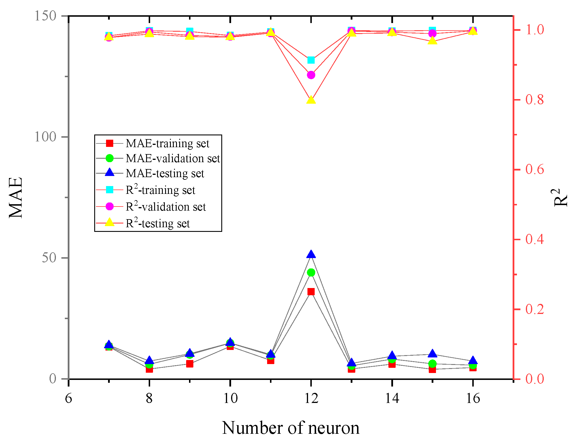
3.2. ANN Algorithm
3.3. XGBoost
3.4. LightGBM
3.5. Model Evaluation Methods
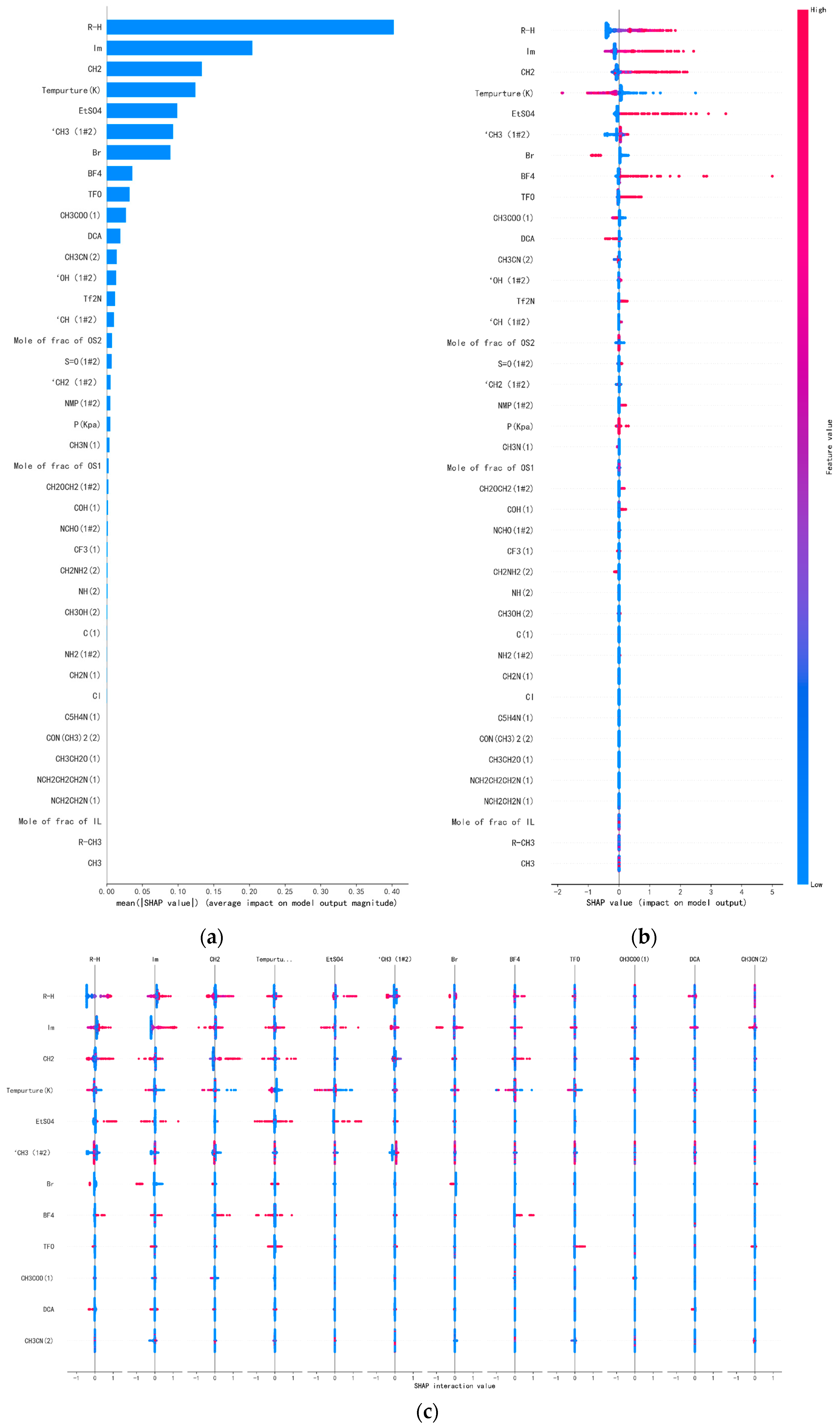
3.6. SHAP Interpretation
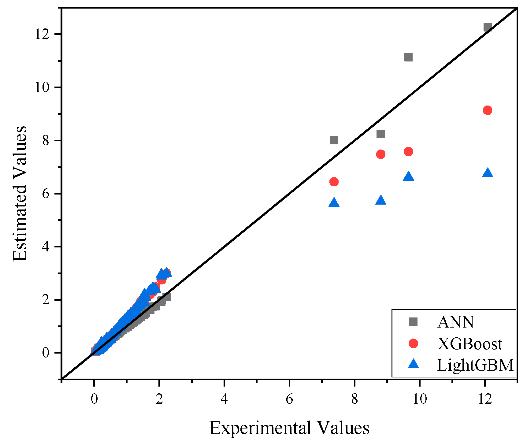
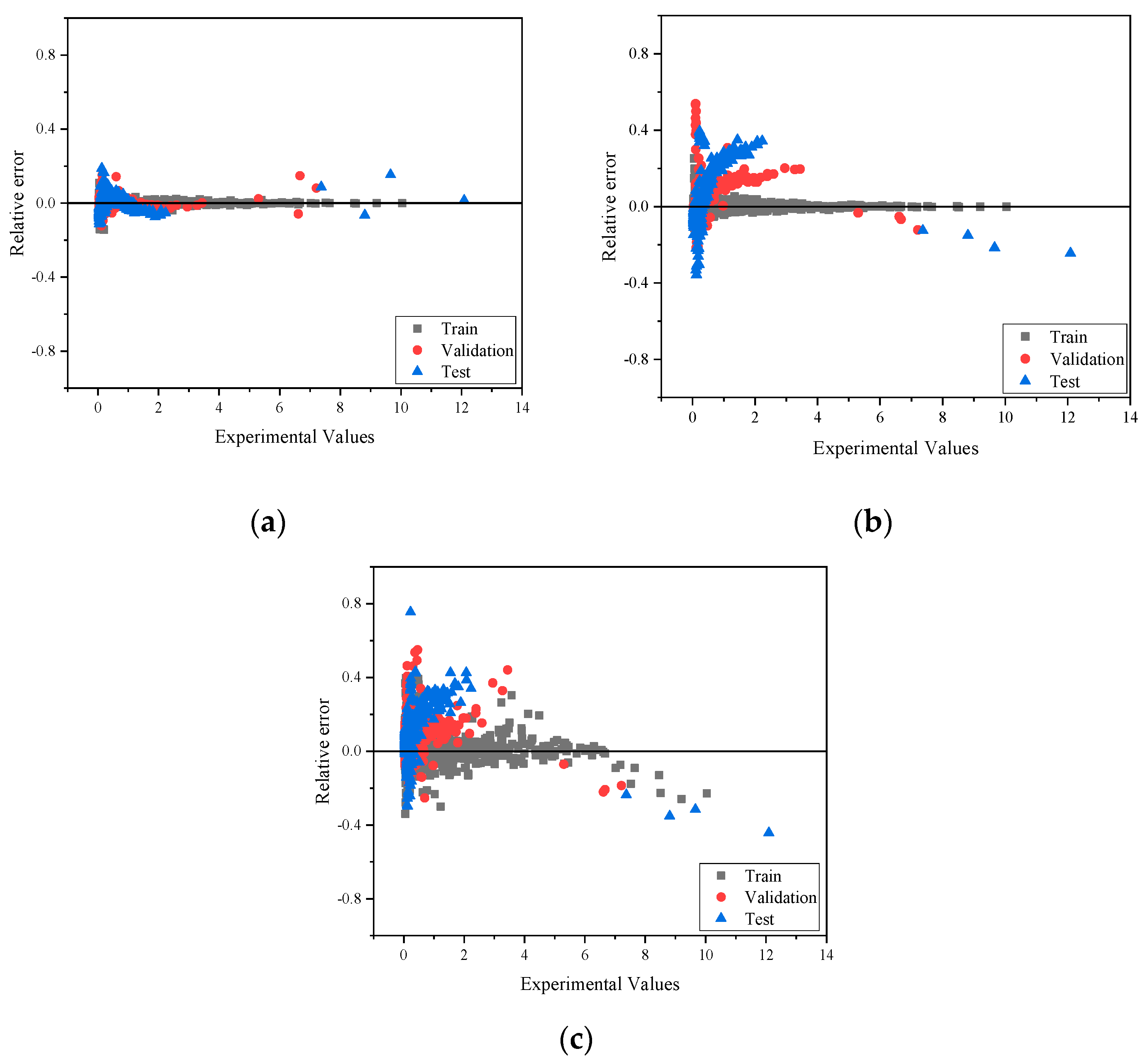
4. Results and Discussions
4.1. Heat Capacity
4.2. Viscosity
4.3. Density
5. Conclusions
Supplementary Materials
Author Contributions
Funding
Data Availability Statement
Conflicts of Interest
References
- Greer, A.J.; Jacquemin, J.; Hardacre, C. Industrial applications of ionic liquids. Molecules 2020, 25, 5207. [Google Scholar] [CrossRef] [PubMed]
- Lei, Z.; Chen, B.; Koo, Y.M.; MacFarlane, D.R. Introduction: Ionic liquids. Chem. Rev. 2017, 117, 6633–6635. [Google Scholar] [CrossRef] [PubMed]
- MacFarlane, D.R.; Forsyth, M.; Izgorodina, E.I.; Abbott, A.P.; Annat, G.; Fraser, K. Industrial applications of ionic liqui liquids. Phys. Chem. Chem. Phys. 2009, 11, 4962–4967. [Google Scholar] [CrossRef] [PubMed]
- Hayes, R.; Warr, G.G.; Atkin, R. Structure and nanostructure in ionic liquids. Chem. Rev. 2015, 115, 6357–6426. [Google Scholar] [PubMed]
- Armstrong, J.P.; Hurst, C.; Jones, R.G.; Licence, P.; Lovelock, K.R.; Satterley, C.J.; Villar-Garcia, I.J. Vapourisation of ionic liquids. Phys. Chem. Chem. Phys. 2007, 9, 982–990. [Google Scholar] [CrossRef] [PubMed]
- Lei, Y.; Du, L.; Liu, X.; Yu, H.; Liang, X.; Kontogeorgis, G.M.; Chen, Y. Natural gas sweetening using tailored ionic liquid-methanol mixed solvent with selective removal of H2S and CO2. Chem. Eng. J. 2023, 476, 146424–146441. [Google Scholar] [CrossRef]
- Lei, Y.; Guo, Z.; Du, L.; Meng, X.; Liu, X.; Wu, X.; Chen, Y. Replacing DMF with ionic liquid in isoprene/n-pentane separation in C5 plants: Solvent design, process optimization, and industrial-scale assessment. Fuel 2024, 357, 130006–130019. [Google Scholar] [CrossRef]
- Lei, Y.; Yu, Z.; Wei, Z.; Liu, X.; Luo, H.; Chen, Y.; Liang, X.; Kontogeorgis, G.M. Energy-efficient separation of propylene/propane by introducing a tailor-made ionic liquid solvent. Fuel 2022, 326, 124930–124941. [Google Scholar] [CrossRef]
- Durga, G.; Mishra, A. Ionic liquids: Industrial applications. In Sustainable Inorganic Chemistry; Wiley: Hoboken, NJ, USA, 2016; pp. 221–234. [Google Scholar]
- Plechkova, N.V.; Seddon, K.R. Applications of ionic liquids in the chemical industry. Chem. Soc. Rev. 2008, 37, 123–150. [Google Scholar] [CrossRef]
- Müller, K.; Albert, J. Contribution of the individual ions to the heat capacity of ionic liquids. Ind. Eng. Chem. Res. 2014, 53, 10343–10346. [Google Scholar] [CrossRef]
- Dai, Z.; Chen, Y.; Liu, C.; Lu, X.; Liu, Y.; Ji, X. Prediction and verification of heat capacities for pure ionic liquids. Chin. J. Chem. Eng. 2021, 31, 169–176. [Google Scholar] [CrossRef]
- Bischoff, L.A.; Drisch, M.; Kerpen, C.; Hennig, P.T.; Landmann, J.; Sprenger, J.A.P.; Bertermann, R.; Grüne, M.; Yuan, Q.; Warneke, J.; et al. Cyanohydridoborate Anions: Synthesis, Salts, and Low-Viscosity Ionic Liquids. Chem.—A Eur. J. 2019, 25, 3560–3574. [Google Scholar] [CrossRef]
- Sepehrnia, M.; Shahsavar, A.; Maleki, H.; Moradi, A. Experimental study on the dynamic viscosity of hydraulic oil HLP 68-Fe3O4-TiO2-GO ternary hybrid nanofluid and modeling utilizing machine learning technique. J. Taiwan Inst. Chem. Eng. 2023, 145, 104841–104856. [Google Scholar] [CrossRef]
- Li, N.; Ma, H.; Wang, T.; Sun, C.; Xia, S. Effect of molecular weight on the properties of water-soluble terpolymers for heavy oil viscosity reduction. J. Taiwan Inst. Chem. Eng. 2023, 144, 104738–104751. [Google Scholar] [CrossRef]
- Amith, W.D.; Araque, J.C.; Margulis, C.J. A pictorial view of viscosity in ionic liquids and the link to nanostructural heterogeneity. J. Phys. Chem. Lett. 2020, 11, 2062–2066. [Google Scholar] [CrossRef]
- Alavianmehr, M.M.; Hosseini, S.M.; Moghadasi, J. Densities of ionic liquids from ion contribution-based equation of state: Electrolyte perturbation approach. J. Mol. Liq. 2014, 197, 287–294. [Google Scholar] [CrossRef]
- Amar, M.N.; Ghriga, M.A.; Hemmati-Sarapardeh, A. Application of gene expression programming for predicting density of binary and ternary mixtures of ionic liquids and molecular solvents. J. Taiwan Inst. Chem. Eng. 2020, 117, 63–74. [Google Scholar] [CrossRef]
- Speiser, J.L.; Miller, M.E.; Tooze, J.; Ip, E. A comparison of random forest variable selection methods for classification prediction modeling. Expert Syst. Appl. 2019, 134, 93–101. [Google Scholar] [CrossRef]
- Gani, R. Group contribution-based property estimation methods: Advances and perspectives. Curr. Opin. Chem. Eng. 2019, 23, 184–196. [Google Scholar] [CrossRef]
- Mjalli, F.S. Mass connectivity index-based density prediction of deep eutectic solvents. Fluid Phase Equilibria 2016, 409, 312–317. [Google Scholar] [CrossRef]
- Zhang, D.; Lin, J.; Peng, Q.; Wang, D.; Yang, T.; Sorooshian, S.; Liu, X.; Zhuang, J. Modeling and simulating of reservoir operation using the artificial neural network, support vector regression, deep learning algorithm. J. Hydrol. 2018, 565, 720–736. [Google Scholar] [CrossRef]
- Alshehri, A.S.; Gani, R.; You, F. Deep learning and knowledge-based methods for computer-aided molecular design-toward a unified approach: State-of-the-art and future directions. Comput. Chem. Eng. 2020, 141, 107005–107063. [Google Scholar] [CrossRef]
- Liu, Q.; Zhang, L.; Liu, L.; Du, J.; Liang, X.; Mao, H.; Meng, Q. GC-COSMO based Reaction Solvent Design with New Kinetic Model using CAMD. Comput. Aided Chem. Eng. 2018, 44, 235–240. [Google Scholar]
- Oster, K.; Jacquemin, J.; Hardacre, C.; Ribeiro, A.; Elsinawi, A. Further development of the predictive models for physical properties of pure ionic liquids: Thermal conductivity and heat capacity. J. Chem. Thermodyn. 2018, 118, 1–15. [Google Scholar] [CrossRef]
- Shi, W.; Maginn E, J. Molecular simulation and regular solution theory modeling of pure and mixed gas absorption in the ionic liquid 1-n-hexyl-3-methylimidazolium bis (trifluoromethylsulfonyl) amide ([hmim][Tf2N]). J. Phys. Chem. B. 2008, 112, 16710–16720. [Google Scholar] [CrossRef] [PubMed]
- Azadfar, R.; Shaabanzadeh, M.; Hashemi-Moghaddam, H.; Mohammadi Nafchi, A. A new simple model to calculate the heat capacity of pure ionic liquids. Phys. Chem. Res. 2020, 8, 139–154. [Google Scholar]
- Macías-Salinas, R.; Gross, J. A viscosity model for pure ionic liquids via the use of a residual-entropy scaling. Fluid Phase Equilibria 2023, 574, 113897–113909. [Google Scholar] [CrossRef]
- Fatehi, M.R.; Raeissi, S.; Mowla, D. Estimation of viscosities of pure ionic liquids using an artificial neural network based on only structural characteristics. J. Mol. Liq. 2017, 227, 309–317. [Google Scholar] [CrossRef]
- Haghbakhsh, R.; Raeissi, S. Two simple correlations to predict viscosities of pure and aqueous solutions of ionic liquids. J. Mol. Liq. 2015, 211, 948–956. [Google Scholar] [CrossRef]
- Paduszynski, K.; Domanska, U. A new group contribution method for prediction of density of pure ionic liquids over a wide range of temperature and pressure. Ind. Eng. Chem. Res. 2012, 51, 591–604. [Google Scholar] [CrossRef]
- Wandschneider, A.; Lehmann, J.K.; Heintz, A. Surface tension and density of pure ionic liquids and some binary mixtures with 1-propanol and 1-butanol. J. Chem. Eng. Data 2008, 53, 596–599. [Google Scholar] [CrossRef]
- Jacquemin, J.; Husson, P.; Padua, A.A.H.; Majer, V. Density and viscosity of several pure and water-saturated ionic liquids. Green Chem. 2006, 8, 172–180. [Google Scholar] [CrossRef]
- Chen, Y.; Kontogeorgis, G.M.; Woodley, J.M. Group contribution based estimation method for properties of ionic liquids. Ind. Eng. Chem. Res. 2019, 58, 4277–4292. [Google Scholar] [CrossRef]
- Chen, Y.; Cai, Y.; Thomsen, K.; Kontogeorgis, G.M.; Woodley, J.M. A group contribution-based prediction method for the electrical conductivity of ionic liquids. Fluid Phase Equilibria 2020, 509, 112462–112478. [Google Scholar] [CrossRef]
- Jouyban, A.; Soleymani, J.; Jafari, F.; Khoubnasabjafari, M.; Acree, W.E. Mathematical representation of viscosity of ionic liquid+ molecular solvent mixtures at various temperatures using the Jouyban–Acree model. J. Chem. Eng. Data 2013, 58, 1523–1528. [Google Scholar] [CrossRef]
- Jouyban, A.; Mirheydari, S.N.; Barzegar-Jalali, M.; Shekaari, H.; Acree, W.E. Comprehensive models for density prediction of ionic liquid+ molecular solvent mixtures at different temperatures. Phys. Chem. Liq. 2020, 58, 309–324. [Google Scholar] [CrossRef]
- Jouyban, A.; Acree, W.E., Jr. A single model to represent physico-chemical properties of liquid mixtures at various temperatures. J. Mol. Liq. 2021, 323, 115054–115065. [Google Scholar] [CrossRef]
- Mirheydari, S.N.; Soleymani, J.; Jouyban-Gharamaleki, V.; Barzegar-Jalali, M.; Jouyban, A.; Shekaari, H. Viscosity prediction of ionic liquid+ molecular solvent mixtures at various temperatures. J. Mol. Liq. 2018, 263, 228–236. [Google Scholar] [CrossRef]
- Wan Normazlan, W.M.D.; Sairi, N.A.; Alias, Y.; Udaiyappan, A.F.; Jouyban, A.; Khoubnasabjafari, M. Composition and temperature dependence of density, surface tension, and viscosity of EMIM DEP/MMIM DMP+ water+ 1-propanol/2-propanol ternary mixtures and their mathematical representation using the Jouyban–acree model. J. Chem. Eng. Data 2014, 59, 2337–2348. [Google Scholar] [CrossRef]
- Gmehling, J. Present status and potential of group contribution methods for process development. J. Chem. Thermodyn. 2009, 41, 731–747. [Google Scholar] [CrossRef]
- Amar, M.N.; Ouaer, H.; Ghriga, M.A. Robust smart schemes for modeling carbon dioxide uptake in metal-organic frameworks. Fuel 2022, 311, 122545–122555. [Google Scholar] [CrossRef]
- Koutsoukos, S.; Philippi, F.; Malaret, F.; Welton, T. A review on machine learning algorithms for the ionic liquid chemical space. Chem. Sci. 2021, 12, 6820–6843. [Google Scholar] [CrossRef] [PubMed]
- Amar, M.N.; Ghriga, M.A.; Ouaer, H. On the evaluation of solubility of hydrogen sulfide in ionic liquids using advanced committee machine intelligent systems. J. Taiwan Inst. Chem. Eng. 2021, 118, 159–168. [Google Scholar] [CrossRef]
- Li, M.; Fu, X.; Li, D. Diabetes prediction based on XGBoost algorithm. In IOP Conference Series: Materials Science and Engineering; IOP Publishing: Bristol, UK, 2020; Volume 768, pp. 072093–072101. [Google Scholar]
- Zhao, W.P.; Li, J.; Zhao, J.; Zhao, D.; Lu, J.; Wang, X. Xgb model: Research on evaporation duct height prediction based on XGboost algorithm. Radioengineering 2020, 29, 81–93. [Google Scholar] [CrossRef]
- Liang, W.; Luo, S.; Zhao, G.; Wu, H. Predicting hard rock pillar stability using GBDT, XGBoost, and LightGBM algorithms. Mathematics 2020, 8, 765. [Google Scholar] [CrossRef]
- Yan, J.; Xu, Y.; Cheng, Q.; Jiang, S.; Wang, Q.; Xiao, Y.; Ma, C.; Yan, J.; Wang, X. LightGBM: Accelerated genomically designed crop breeding through ensemble learning. Genome Biol. 2021, 22, 1–24. [Google Scholar] [CrossRef]
- Nohara, Y.; Matsumoto, K.; Soejima, H.; Nakashima, N. Explanation of machine learning models using improved shapley additive explanation. In Proceedings of the 10th ACM International Conference on Bioinformatics, Computational Biology and Health Informatics, Niagara Falls, NY, USA, 7–10 September 2019; p. 546. [Google Scholar]
- Wang, D.; Thunéll, S.; Lindberg, U.; Jiang, L.; Trygg, J.; Tysklind, M. Towards better process management in wastewater treatment plants: Process analytics based on SHAP values for tree-based machine learning methods. J. Environ. Manag. 2022, 301, 113941–113953. [Google Scholar] [CrossRef]
- Sharma, V.K.; Bhagour, S.; Solanki, S.; Sharma, D. Excess heat capacities of (binary+ ternary) mixtures containing [emim][BF4] and organic liquids. J. Chem. Thermodyn. 2014, 79, 19–32. [Google Scholar] [CrossRef]
- Darolia, P.J.; Malik, S.; Garg, S.; Sharma, V.K. Molar heat capacities and excess molar heat capacities of mixtures containing ionic liquids and cyclic amides. Chem. Data Collect. 2022, 41, 100939–100955. [Google Scholar] [CrossRef]
- Sharma, V.K.; Kataria, J.; Sharma, D. Excess heat capacities of mixtures containing 1-ethyl-3-methylimidazolium tetrafluoroborate, lactams and cyclic alkanones. J. Therm. Anal. Calorim. 2015, 121, 777–796. [Google Scholar]
- Anwar, N.; Riyazuddeen. Excess molar volumes, excess molar isentropic compressibilities, viscosity deviations, and activation parameters for 1-ethyl-3-methyl-imidazolium trifluoro-methanesulfonate+ dimethyl sulfoxide and/or acetonitrile at T= 298.15 to 323.15 K and P= 0.1 MPa. J. Chem. Eng. Data. 2018, 63, 269–289. [Google Scholar] [CrossRef]
- Anwar, N. Effect of composition and temperature variations on thermophysical properties of binary and ternary mixtures of 1-ethyl-3-methylimidazolium ethylsulfate with 1-butanol and/or methanol. Fluid Phase Equil. 2017, 437, 127–139. [Google Scholar] [CrossRef]
- Kermanpour, F.; Sharifi, T. Measurement and correlation of the excess properties of ternary mixture of {x1 [Hmim][BF4]+ x21-propanol+ x32-propanol} at different temperatures. J. Chem. Eng. Data. 2014, 59, 1922–1929. [Google Scholar] [CrossRef]
- Shekaari, H.; Zafarani-Moattar M, T.; Mirheydari S, N. Density, viscosity, speed of sound, and refractive index of a ternary solution of aspirin, 1-butyl-3-methylimidazolium bromide, and acetonitrile at different temperatures T = (288.15 to 318.15) K. J. Chem. Eng. Data. 2015, 60, 1572–1583. [Google Scholar]
- Shekaari, H.; Zafarani-Moattar M, T.; Mirheydari S, N. Thermodynamic study of aspirin in the presence of ionic liquid, 1-hexyl-3-methylimidazolium bromide in acetonitrile at T = (288.15 to 318.15) K. J. Mol. Liq. 2015, 209, 138–148. [Google Scholar] [CrossRef]
- Anwar, N.; Urooj, F. Effect of co-solvent and temperature on interactions in 1-ethyl-3-methylimidazolium trifluoromethanesulfonate+ ethylene glycol or/and N, N-dimethylformamide, and ethylene glycol+ N, N-dimethylformamide mixtures: Measurement of thermophysical properties. J. Mol. Liq. 2018, 265, 121–134. [Google Scholar] [CrossRef]
- Fatima, U.; Riyazuddeen; Anwar, N. Effect of solvents and temperature on interactions in binary and ternary mixtures of 1-butyl-3-methylimidazolium trifluoromethanesulfonate with acetonitrile or/and N, N-dimethylformamide. J. Chem. Eng. Data 2018, 63, 4288–4305. [Google Scholar]
- Fatima, U.; Riyazuddeen ; Dhakal, P.; Shah, J.K. Comparative study of influence of ethanol and 2, 2, 2-trifluoroethanol on thermophysical properties of 1-ethyl-3-methylimidazolium dicyanamide in binary mixtures: Experimental and MD simulations. J. Chem. Eng. Data 2020, 66, 101–115. [Google Scholar]
- Andreatta, A.E.; Arce, A.; Rodil, E.; Soto, A. Physical properties of binary and ternary mixtures of ethyl acetate, ethanol, and 1-octyl-3-methyl-imidazolium bis (trifluoromethylsulfonyl) imide at 298.15 K. J. Chem. Eng. Data 2009, 54, 1022–1028. [Google Scholar] [CrossRef]
- Andreatta, A.E.; Arce, A.; Rodil, E.; Soto, A. Physical and excess properties of (methyl acetate+ methanol+ 1-octyl-3-methyl-imidazolium bis (trifluoromethylsulfonyl) imide) and its binary mixtures at T = 298.15 K and atmospheric pressure. J. Chem. Thermodyn. 2009, 41, 1317–1323. [Google Scholar]
- Andreatta, A.E.; Arce, A.; Rodil, E.; Soto, A. Physico-chemical properties of binary and ternary mixtures of ethyl acetate+ ethanol+ 1-butyl-3-methyl-imidazolium bis (trifluoromethylsulfonyl) imide at 298.15 K and atmospheric pressure. J. Solution Chem. 2010, 39, 371–383. [Google Scholar] [CrossRef]
- Andreatta, A.E.; Francisco, M.; Rodil, E.; Soto, A.; Arce, A. Isobaric vapour–liquid equilibria and physical properties for isopropyl acetate+ isopropanol+ 1-butyl-3-methyl-imidazolium bis (trifluoromethylsulfonyl) imide mixtures. Fluid Phase Equil. 2011, 300, 162–171. [Google Scholar] [CrossRef]
- Andreatta, A.E.; Arce, A.; Rodil, E.; Soto, A. Physical properties and phase equilibria of the system isopropyl acetate+ isopropanol+ 1-octyl-3-methyl-imidazolium bis (trifluoromethylsulfonyl) imide. Fluid Phase Equil. 2010, 287, 84–94. [Google Scholar] [CrossRef]
- Shekaari, H.; Bezaatpour, A.; Khoshalhan, M. Thermophysical properties of ionic liquid, 1-hexyl-3-methylimidazolum bromide + N-N′bis(2-pyridylmethylidene)-1,2-diiminoethane (BPIE) Schiff base + N,N-dimethylformamide solutions. Thermochim. Acta 2012, 52, 67–74. [Google Scholar] [CrossRef]
- Shekaari, H.; Kazempour, A.; Khoshalhan, M. Effect of N, N′-bis (2-pyridylmethylidene)-1, 2-diiminoethane Schiff base (BPIE) on the thermodynamic properties of the ionic liquid 1-hexyl-3-methylimidazolium chloride in N, N-dimethylacetamide solvent at T = 298.15 K. J. Chem. Thermodyn. 2015, 81, 131–135. [Google Scholar] [CrossRef]
- Shekaari, H.; Kazempour, A.; Khoshalhan, M. Densities and Viscosities of Ternary N, N′-Bis (2-pyridylmethylidene)-1, 2-diiminoethane Schiff Base+ Imidazolium Based Ionic Liquids+ Acetonitrile Solutions at T = (298.15 to 313.15) K. J. Chem. Eng. Data 2015, 60, 1106–1118. [Google Scholar] [CrossRef]
- Shekaari, H.; Bezaatpour, A.; Khoshalhan, M. Effect of N, N′-Bis (2-pyridylmethylidene)-1, 2-diiminoethane (BPIE) Schiff Base on the thermophysical properties of ionic liquids in N, N-dimethylformamide solutions at 298.15 K. J. Chem. Eng. Data 2011, 56, 4164–4172. [Google Scholar] [CrossRef]
- Arce, A.; Rodil, E.; Soto, A. Volumetric and viscosity study for the mixtures of 2-ethoxy-2-methylpropane, ethanol, and 1-ethyl-3-methylimidazolium ethyl sulfate ionic liquid. J. Chem. Eng. Data 2006, 51, 1453–1457. [Google Scholar] [CrossRef]
- Foo, C.K.; Leo, C.Y.; Aramesh, R.; Aroua, M.K.; Aghamohammadi, N.; Shafeeyan, M.S.; Shamiri, A. Density and viscosity of aqueous mixtures of N-methyldiethanolamines (MDEA), piperazine (PZ) and ionic liquids. J. Mol. Liq. 2015, 209, 596–602. [Google Scholar] [CrossRef]
- Shekaari, H.; Bezaatpour, A.; Elhami-Kalvanagh, R. Thermodynamic properties of salophen schiff base+ ionic liquid ([C n mIm][Br])+ dimethylformamide ternary mixtures at 298.15 K. J. Chem. Eng. Data 2012, 57, 345–351. [Google Scholar] [CrossRef]
- Shekaari, H.; Bezaatpour, A.; Elhami, R. Volumetric and Viscometric Studies of N, N′-Bis (salicylaldehyde)-1, 3-diaminopropane Schiff Base (Salpr) in Ionic Liquid+ DMF solutions. J. Solut. Chem. 2012, 41, 516–524. [Google Scholar] [CrossRef]
- Shekaari, H.; Elhami-Kalvanagh, R.; Bezaatpour, A. Effect of ionic liquid on the solvation behavior of nonaqueous N, N′-salicylidenephenylediamine Schiff base (Salophen) solutions at 298.15 K. J. Chem. Thermodyn. 2013, 64, 58–64. [Google Scholar] [CrossRef]
- Kermanpour, F.; Iloukhani, H.; Javanshad, M. Measurement and modeling the excess properties of binary and ternary mixtures containing [Hmim][BF4], 2-methyl-2-propanol, and propylamin compounds at 298.15 K using PFP theory. J. Mol. Liq. 2013, 188, 22–27. [Google Scholar] [CrossRef]
- Ebrahiminejadhasanabadi, M.; Nelson, W.M.; Naidoo, P.; Mohammadi, A.H.; Ramjugernath, D. Investigation of mixed MEA-based solvents featuring ionic liquids and NMP for CO2 capture: Experimental measurement of CO2 solubility and thermophysical properties. J. Chem. Eng. Data 2021, 66, 899–914. [Google Scholar] [CrossRef]
- Ebrahiminejadhasanabadi, M.; Nelson, W.M.; Naidoo, P.; Mohammadi, A.H.; Ramjugernath, D. Experimental measurements of CO2 solubility, viscosity, density, sound velocity and evaporation rate for 2-(2-aminoethoxy) ethanol (DGA)+ 1-methylpyrrolidin-2-one (NMP)/water+ ionic liquid systems. Fluid Phase Equil. 2022, 559, 113475–113488. [Google Scholar] [CrossRef]
- Malik, S.; Gupta, H.; Sharma V, K. Molecular interactions in ternary liquid mixtures containing alkyl imidazolium tetrafluroborates and cyclic ketones: Excess molar volumes and excess isentropic compressibilities. Chem. Data Collect. 2021, 31, 100603–100611. [Google Scholar] [CrossRef]
- Deenadayalu, N.; Bahadur, I.; Hofman, T. Ternary excess molar volumes of {methyltrioctylammonium bis (trifluoromethylsulfonyl) imide+ ethanol+ methyl acetate, or ethyl acetate} systems at T=(298.15, 303.15, and 313.15) K. J. Chem. Thermodyn. 2010, 42, 726–733. [Google Scholar] [CrossRef]
- Sharma, V.K.; Solanki, S.; Bhagour, S.; Sharma, D. Topological investigations of thermodynamic properties of ionic liquid mixtures: Excess molar volumes and excess isentropic compressibilities. J. Mol. Liq. 2013, 188, 258–271. [Google Scholar] [CrossRef]
- Fatima, U.; Montes-Campos, H.; Varela L, M. Experimental and MD simulation investigation on thermophysical properties of binary/ternary mixtures of 1-butyl-3-methylimidazolium trifluoromethanesulfonate with molecular solvents. J. Mol. Liq. 2020, 302, 112481–112537. [Google Scholar] [CrossRef]
- Rafiee H, R.; Frouzesh, F. Volumetric properties for binary and ternary mixtures of allyl alcohol, 1, 3-dichloro-2-propanol and 1-ethyl-3-methyl imidazolium ethyl sulfate [Emim][EtSO4] from T= 298.15 to 318.15 K at ambient pressure. Thermochim. Acta 2015, 611, 36–46. [Google Scholar] [CrossRef]
- Singh, S.; Bahadur, I.; Redhi, G.G.; Karlapudi, S.; Ramjugernath, D.; Hofman, T.; Ebenso, E.E. Cibulka correlation for ternary excess/deviation properties of {[C2mim][EtSO4](x1)+ acetic or propionic acid (x2)+ acetonitrile (x3)} systems at different temperatures. J. Chem. Thermodyn. 2017, 107, 153–162. [Google Scholar] [CrossRef]
- Masilo, K.; Bahadur, I.; Paredes M L, L. Measurement and Modeling of Thermodynamic Properties for Ternary Mixtures Containing 1-Butyl-3-methylimidazolium-Based Ionic Liquids with Acetophenone and Acetic or Propionic Acid. J. Chem. Eng. Data 2021, 66, 4368–4383. [Google Scholar] [CrossRef]
- Sharma, V.K.; Bhagour, S.; Solanki, S.; Rohilla, A. Thermodynamic properties of ternary mixtures containing ionic liquids and organic solvents. J. Chem. Eng. Data 2013, 58, 1939–1954. [Google Scholar] [CrossRef]
- Sharma V, K.; Solanki, S.; Bhagour, S. Thermodynamic properties of ternary mixtures containing ionic liquid and organic liquids: Excess molar volume and excess isentropic compressibility. J. Chem. Eng. Data 2014, 59, 1140–1157. [Google Scholar] [CrossRef]
- Singh, S.; Bahadur, I.; Ebenso E, E. Thermodynamic properties of ternary mixture {[C4mim][SCN]+ acetic or propionic acid+ acetonitrile} over the temperature range of (293.15–313.15) K. J. Chem. Thermodyn. 2019, 138, 321–331. [Google Scholar] [CrossRef]
- Bahadur, I.; Deenadayalu, N.; Tywabi, Z.; Sen, S.; Hofman, T. Volumetric properties of ternary (IL+ 2-propanol or 1-butanol or 2-butanol+ ethyl acetate) systems and binary (IL+ 2-propanol or 1-butanol or 2-butanol) and (1-butanol or 2-butanol+ ethyl acetate) systems. J. Chem. Thermodyn. 2012, 49, 24–38. [Google Scholar] [CrossRef]
- Sharma V, K.; Kataria, J.; Solanki, S. Thermodynamic properties of ternary mixtures containing 1-ethyl-3-methylimidazolium tetrafluoroborate with cyclic amides and cyclopentanone or cyclohexanone at T = (293.15, 298.15, 303.15 and 308.15) K. J. Chem. Thermodyn. 2015, 86, 43–56. [Google Scholar] [CrossRef]
- Zhu, Q.; Wang, C.; Yin, J.; Li, H.; Jiang, W.; Liu, J.; Zhu, W. Efficient and remarkable SO2 capture: A discovery of imidazole-based ternary deep eutectic solvents. J. Mol. Liq. 2021, 330, 11559–11568. [Google Scholar] [CrossRef]
- Abu-Eishah S, I.; Dowaidar A, M. Liquid− liquid equilibrium of ternary systems of cyclohexane+(benzene,+ toluene,+ ethylbenzene, or+ o-xylene)+ 4-methyl-N-butyl pyridinium tetrafluoroborate ionic liquid at 303.15 K. J. Chem. Eng. Data 2008, 53, 1708–1712. [Google Scholar] [CrossRef]
- Bastos, P.D.; Oliveira, F.S.; Rebelo, L.P.; Pereiro, A.B.; Marrucho, I.M. Separation of azeotropic mixtures using high ionicity ionic liquids based on 1-ethyl-3-methylimidazolium thiocyanate. Fluid Phase Equil. 2015, 389, 48–54. [Google Scholar] [CrossRef]
- Hu, X.; Li, Y.; Cui, D.; Chen, B. Separation of ethyl acetate and ethanol by room temperature ionic liquids with the tetrafluoroborate anion. J. Chem. Eng. Data 2008, 53, 427–433. [Google Scholar] [CrossRef]


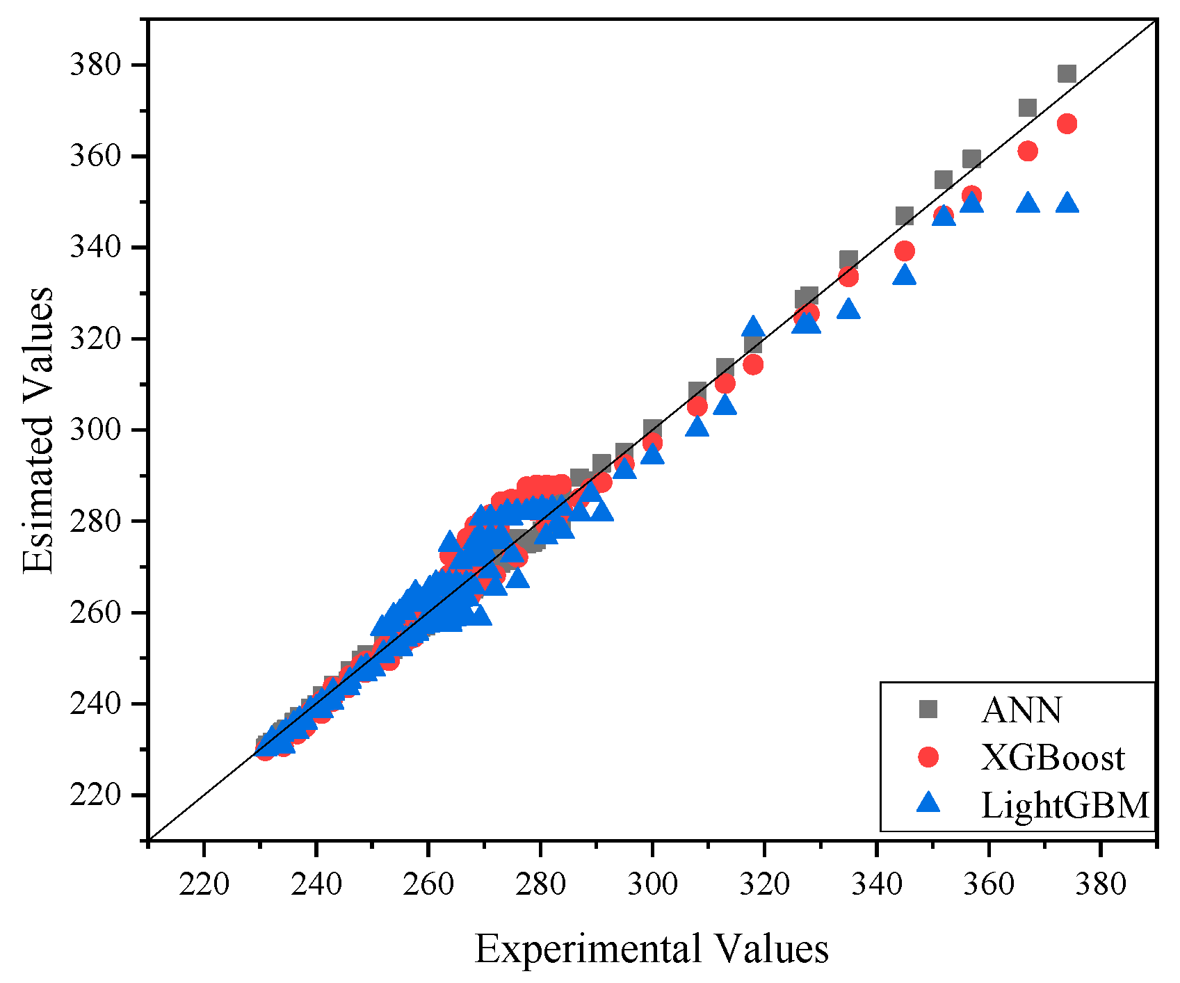
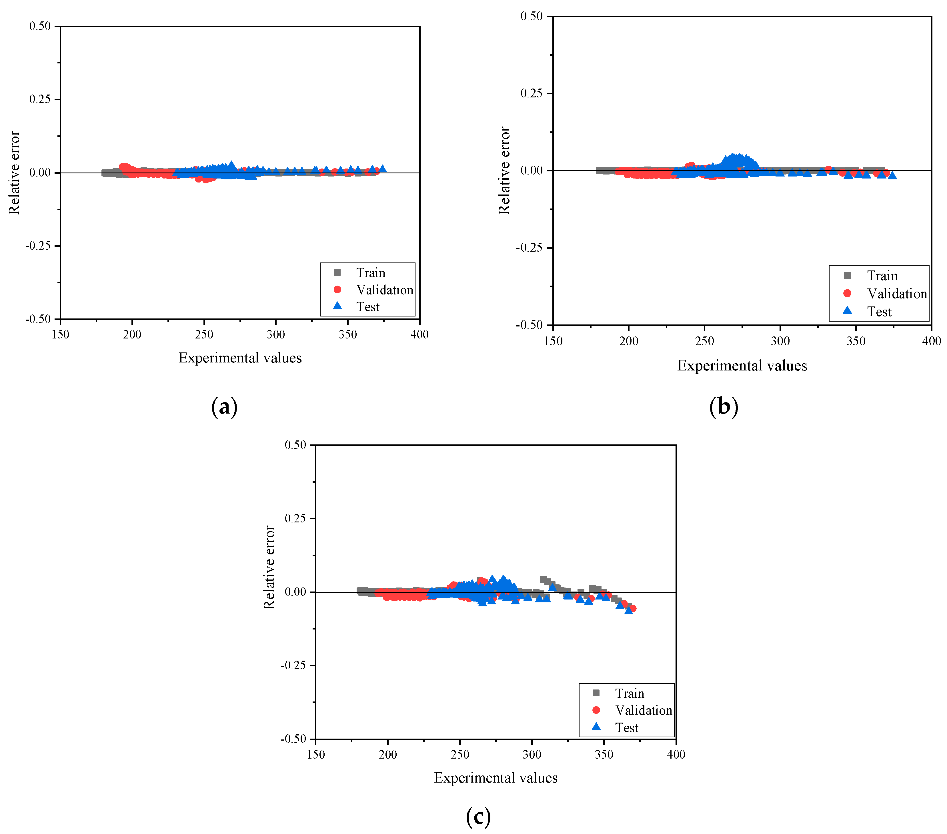

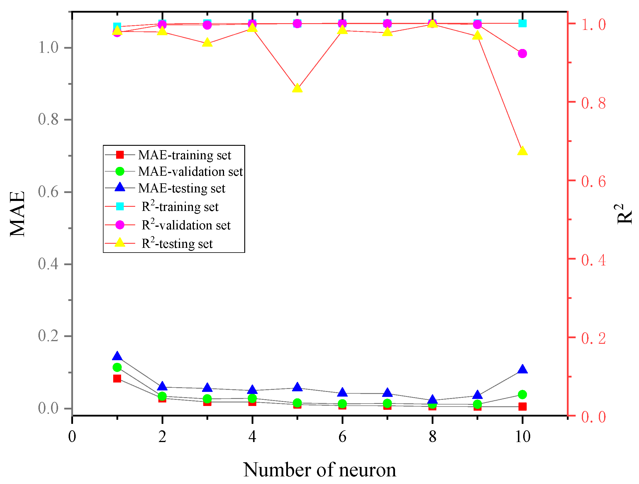
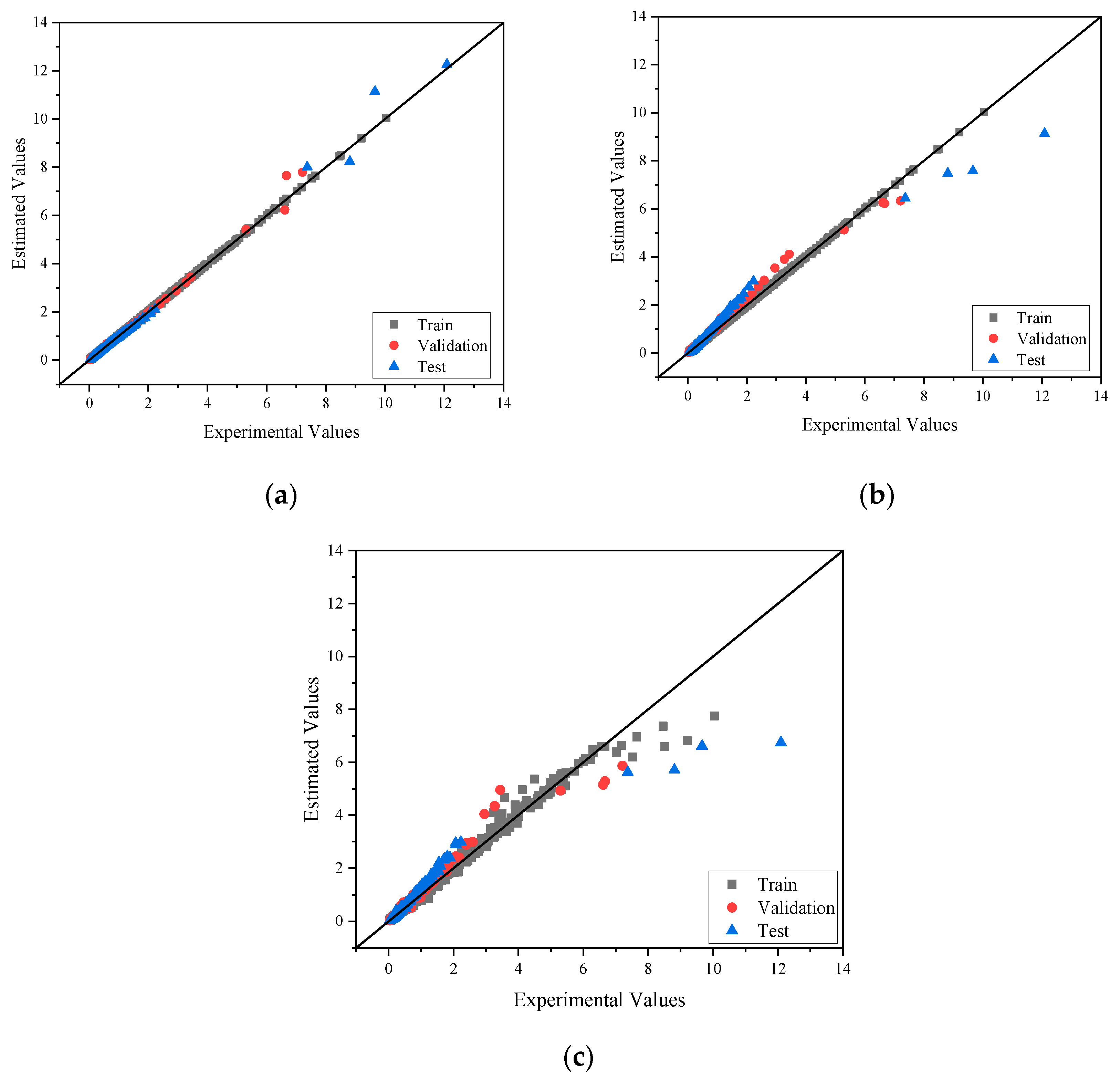
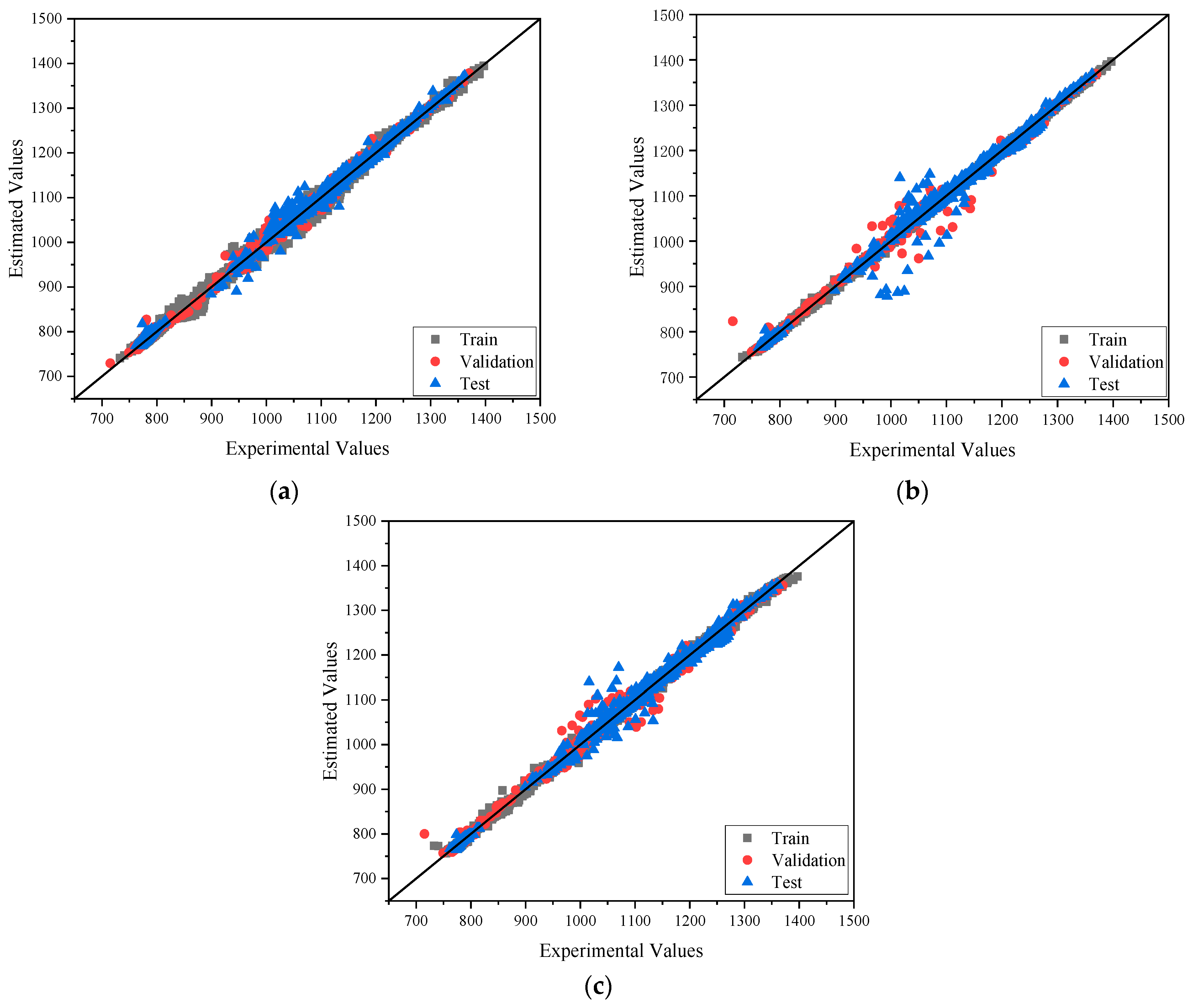

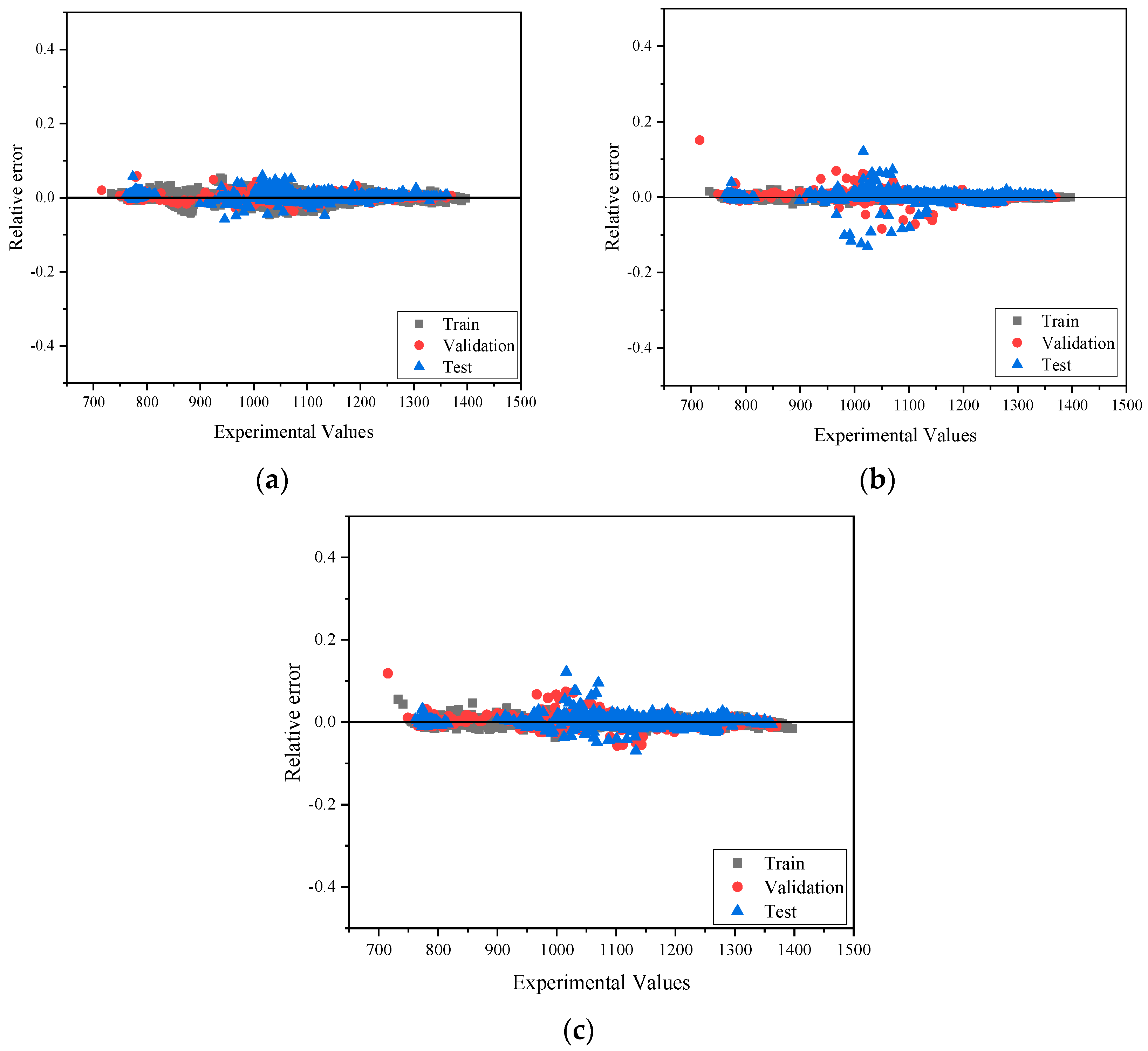

| IL-OS (1)-OS (2) | Temperature (K) | Heat Capacity (J·K−1·mol−1) |
|---|---|---|
| [EMIM][BF4]-(N-methylpyrrolidone)-pyridine [51] | 293.15–308.15 | 189.9–270 |
| [EMIM][BF4]-(2-pyrrolidinone)-pyridine [51] | 293.15–308.15 | 190.6–269 |
| [BMMIM][BF4]-(N-methylpyrrolidone)-(2-pyrrolidinone) [52] | 293.15–308.15 | 196.1–374 |
| [EMIM][BF4]-(N-methylpyrrolidone)-(2-pyrrolidinone) [52] | 293.15–308.15 | 191–291 |
| [EMIM][BF4]-(N-methylpyrrolidone)-cyclohexanone [53] | 293.15–308.15 | 181.2–269.5 |
| [EMIM][BF4]-(N-methylpyrrolidone)-cyclopentanone [53] | 293.15–308.15 | 180.8–266.8 |
| [EMIM][BF4]-cyclohexanone-(2-pyrrolidinone) [53] | 293.15–308.15 | 184–272.7 |
| [EMIM][BF4]-(2-pyrrolidinone)-cyclopentanone [53] | 293.15–308.15 | 183.6–283.8 |
| IL-OS (1)-OS (2) | Temperature (K) | Viscosity (mPa·s) |
|---|---|---|
| [EMIM][TFO]-(dimethyl sulfoxide)-acetonitrile [54] | 298.15–323.15 | 0.28–46 |
| [EMIM][EtSO4]-(butan-1-ol)-methanol [55] | 298.15–323.15 | 1.19–84.6 |
| [HMIM][BF4]-(propan-2-ol)-(propan-1-ol) [56] | 298.15–333.15 | 1.06–153.8 |
| [BMIM][Br]-(2-acetoxybenzoic acid)-acetonitrile [57] | 288.15–318.15 | 0.289–0.48 |
| [HMIM][Br]-(2-acetoxybenzoic acid)-acetonitrile [58] | 288.15–318.15 | 0.292–0.462 |
| [EMIM][TFO]-dimethylformamide-(1,2-ethanediol) [59] | 298.15–323.15 | 0.89–29.3 |
| [BMIM][TFO]-dimethylformamide-(acetonitrile) [60] | 298.15–323.15 | 0.39–39.67 |
| [EMIM][DCA]-(2,2,2-trifluoroethanol)-ethanol [61] | 298.15–323.15 | 0.1–8.84 |
| [OMIM][Tf2N]-ethyl acetate-ethanol [62] | 298.15–323.15 | 0.498–60.11 |
| [OMIM][Tf2N]-methyl ethanoate-methanol [63] | 298.15–323.15 | 0.456–70.2 |
| [BMIM][TF2N]-ethyl acetate-ethanol [64] | 298.15–323.15 | 0.523–34.1 |
| [BMIM][TF2N]-isopropyl acetate-(propan-2-ol) [65] | 298.15 | 0.674–34.77 |
| [OMIM][TF2N]-isopropyl acetate-(propan-2-ol) [66] | 298.15 | 0.487–62.4 |
| [HMIM][Br]-(1,2-Ethanediamine)-DMF [67] | 298.15 | 0.861–1.076 |
| [HMIM][Cl]-(1,2-Ethanediamine)-(N,N-DMF) [68] | 298.15 | 0.989–1.234 |
| [C3MIM][Br]-(1,2-Ethanediamine)-acetonitrile [69] | 298.15 | 0.343–0.4198 |
| [C5MIM][Br]-(1,2-Ethanediamine)-acetonitrile [69] | 298.15 | 0.343–0.4391 |
| [HMIM][Br]-(1,2-Ethanediamine)-acetonitrile [69] | 298.15 | 0.343–0.442 |
| [HMIM][Cl]-(1,2-Ethanediamine)-acetonitrile [69] | 298.15 | 0.343–0.409 |
| [C5MIM][Br]-(1,2-Ethanediamine)-DMF [70] | 298.15 | 0.877–1.05 |
| [C3MIM][Br]-(1,2-Ethanediamine)-DMF [70] | 298.15 | 0.88–1.036 |
| [EMIM][EtSO4]-(tert-amyl ethyl ether)-ethanol [71] | 298.15 | 0.878–100.4 |
| [BMIM][BF4]-MDEA-piperazine [72] | 313.15–363.15 | 0.443–1.77 |
| [BMIM][DCA]-MDEA-piperazine [72] | 313.15–363.15 | 0.5–1.97 |
| [EMIM][TFO]-MDEA-piperazine [72] | 313.15–363.15 | 0.54–1.8 |
| [C3MIM][Br]-bisphenol A-DMF [73] | 298.15 | 0.802–0.993 |
| [C5MIM][Br]-H2pbp-DMF [74] | 298.15 | 0.831–1.179 |
| [BMIM][Br]-bisphenol A-(N,N-DMF) [75] | 298.15 | 0.954–1.308 |
| [BMIM][Br]-bisphenol A-dimethyl sulfoxide [75] | 298.15 | 1.998–2.53 |
| [HMIM][BF4](tert-Butanol)-(propan-1-amine) [76] | 298.15 | 0.723–120.9 |
| [BMIM][TF2N]-(N-methylpyrrolidone)-Olamine [77] | 293.15–333.15 | 1.848–6.416 |
| [BMIM][TF2N]-DGA-(N-methylpyrrolidone) [78] | 293.15 | 2.335–12.21 |
| [C5MIM][Br]-bisphenol A-(DMF) [79] | 298.15 | 0.827–0.962 |
| IL-OS (1)-OS (2) | Temperature (K) | Specific Density Liquid (kg·m−3) |
|---|---|---|
| [EMIM][TFA]-dimethyl sulfoxide-acetonitrile [54] | 298.15–323.15 | 749.2–1379.9 |
| [HMIM][Br]-(1,2-Ethanediamine)-DMF [67] | 298.15–313.15 | 930.63–961.97 |
| [HMIM][Br]-(1,2-Ethanediamine)-acetonitrile [69] | 298.15–313.15 | 752.5–801.9 |
| [C3MIM][Br]-(1,2-Ethanediamine)-acetonitrile [69] | 298.15–313.15 | 755.4–802 |
| [HMIM][Cl]-(1,2-Ethanediamine)-acetonitrile [69] | 298.15–313.15 | 755.3–796.1 |
| [C5MIM][Br]-(1,2-Ethanediamine)-acetonitrile [69] | 298.15–313.15 | 752.5–805.2 |
| [EMIM][EtSO4]-(butan-1-ol)(methanol [55] | 298.15–323.15 | 824.2–1225.1 |
| [HMIM][BF4]-(propan-1-ol)(propan-2-ol) [56] | 293.15–333.15 | 846.62–1130.62 |
| [BMIM][Br]-(2-acetoxybenzoic acid)-acetonitrile [57] | 288.15–318.15 | 754.851–826.45 |
| [HMIM][Br]-(2-acetoxybenzoic acid)-acetonitrile [58] | 288.15–318.15 | 763.7–828.4 |
| [BMIM][TFO]-DMF-(1,2-ethanediol) [59] | 298.15–323.15 | 965.93–1356.6 |
| [EMIM][TFO]-DMF-acetonitrile [60] | 298.15–323.15 | 817.7–1263.9 |
| [EMIM][DCA]-(2,2,2-trifluoroethanol)-ethanol [61] | 298.15–323.15 | 1103.4–1340.1 |
| [EMIM][BF4]-cyclohexanone-cyclopentanone [79] | 293.15–308.15 | 1012.4–1283.9 |
| [BMMIM][BF4]-cyclohexanone-cyclopentanone [79] | 293.15–308.15 | 957.9–1193.5 |
| [BMIM][BF4]-cyclohexanone-cyclopentanone [79] | 293.15–308.15 | 995.6–1203.1 |
| [N1,8,8,8][BEI]-methyl ethanoate-ethanol [80] | 298.15–313.15 | 831.2–1104.6 |
| [N1,8,8,8][BEI]-ethyl acetate-ethanol [80] | 298.15–313.15 | 885.8–1105.1 |
| [EMIM][BF4]-(2-methylaniline)-(N-methylaniline) [81] | 293.15–308.15 | 1038.77–1226 |
| [EMIM][BF4]-(2-methylaniline)-aniline [81] | 293.15–308.15 | 1042.3–1243.7 |
| [BMIM][TFO]-dimethyl sulfoxide-(1,2-ethanediol) [82] | 298.15–323.15 | 1092.9–1270.5 |
| [EMIM][EtSO4]-(1,3-dichloro-2-propanol)-(2-propenol) [83] | 298.15–318.15 | 899.6–1333 |
| [EMIM][EtSO4]-acetic acid-acetonitrile [84] | 293.15–313.15 | 962.8–1229.4 |
| [BMIM][BF4]-propanoic acid-acetophenone [85] | 293.15–333.15 | 974–1191 |
| [EMIM][BF4]-(N-methylpyrrolidone)-pyridine [86] | 293.15–308.15 | 1085.8–1247.2 |
| [EMIM][BF4]-(2-pyrrolidinone)-pyridine [86] | 293.15–308.15 | 1148.1–1253.8 |
| [EMIM][BF4]-(2-methylaniline)-pyridine [87] | 293.15–308.15 | 1061.7–1238.3 |
| [EMIM][BF4]-(2-methylaniline)-(4-methylpyridine) [87] | 293.15–308.15 | 1041.9–1241.2 |
| [EMIM][BF4]-(2-methylaniline)-(3-methylpyridine) [87] | 293.15–308.15 | 1040.9–1234.1 |
| [BMIM][SCN]-propanoic acid-acetonitrile [88] | 293.15–313.15 | 908.9–1068.3 |
| [BMIM][PF6]-acetophenone-acetic acid [85] | 293.15–333.15 | 1021–1397 |
| [BMIM][BF4]-acetophenone-acetic acid [85] | 293.15–333.15 | 1004–1177 |
| [BMIM][SCN]-acetic acid-acetonitrile [88] | 293.15–313.15 | 924.8–1071.4 |
| [N1,8,8,8][BEI]-(butan-1-ol)-ethyl acetate [89] | 298.15–313.15 | 855–1105.4 |
| [N1,8,8,8][BEI]-(butan-2-ol)-ethyl acetate [89] | 298.15–313.15 | 855.3–1105.4 |
| [EMIM][BF4]-(N-methylpyrrolidone)-cyclopentanone [90] | 293.15–308.15 | 1089.1–1241.4 |
| [EMIM][BF4]-(2-pyrrolidinone)-cyclopentanone [91] | 293.15–308.15 | 1119.4–1249.5 |
| [EMIM][BF4]-(2-pyrrolidinone)-cyclohexanone [90] | 293.15–308.15 | 1133.2–1245.7 |
| [EMIM][BF4]-(N-methylpyrrolidone)-cyclohexanone [90] | 293.15–308.15 | 1036.4–1189.8 |
| [N1,8,8,8][BEI]-ethyl acetate-(propan-2-ol) [89] | 298.15–313.15 | 833.9–1102 |
| [OMIM][BEI]-methyl ethanoate-methanol [63] | 298.15 | 945.61–1313.39 |
| [EMIM][EtSO4]-propanoic acid-acetonitrile [84] | 293.15–313.15 | 958.4–1196.6 |
| [N1,8,8,8][BEI]-methyl ethanoate-methanol [80] | 298.15–313.15 | 926.7–1102.9 |
| [EMIM][EtSO4]-(tert-amyl ethyl ether)-ethanol [71] | 298.15 | 785.22–1238.8 |
| [C5MIM][Br]-salnaph-DMF [73] | 298.15 | 944.1–980.9 |
| [EMIM][Cl]-(di(2-aminoethyl)amine)-(1,2-ethanediol) [91] | 293–353 | 1013.4–1104.9 |
| [BMPY][BF4]-(1,2-dimethylbenzene)-cyclohexane [92] | 303.15 | 7.652–11.634 |
| [EMIM][SCN]-heptane-ethanol [93] | 298.15 | 675.41–1113 |
| [EMMIM][BF4]-ethyl acetate-ethanol [94] | 298.15 | 822–1070 |
| [HEMMIM][BF4]-ethyl acetate-ethanol [94] | 298.15 | 817–1070 |
| [HMIM][BF4]-(2-methylpropan-2-ol)-(propan-1-amine) [76] | 298 | 774.36–1126.62 |
| [HEMIM][BF4]-ethyl acetate-ethanol [94] | 298.15 | 805–1205 |
| [EMIM][BF4]-ethyl acetate-ethanol [94] | 298.15 | 819–1112 |
| Names | Abbreviations | Names | Abbreviations |
|---|---|---|---|
| IL-Cations | IL-Anions | ||
| imidazolium | [Im] | tetrafluoroborate | [BF4] |
| IL-Substituents | OS-Functional groups | ||
| Methyl | CH3 | methylene | CH2 |
| methyl attached to cation cores | R-CH3 | carbon monoxide | CO |
| methylene | CH2 | amino | NH2 |
| hydrogen attached to cation cores | R-H | n-methylpyrrolidone | NMP |
| pyridine | C5H5N | ||
| Names | Abbreviations | Names | Abbreviations |
|---|---|---|---|
| IL-Cations | IL-Anions | ||
| imidazolium | [Im] | trifluoromethanesulfonate | [TFO] |
| IL-Substituents | ethyl sulfate | [EtSO4] | |
| Methyl | CH3 | tetrafluoroborate | [BF4] |
| methyl attached to cation cores | R-CH3 | bromide | [Br] |
| methylene | CH2 | dimethylphosphate | [DMPO4] |
| hydrogen attached to cation cores | R-H | ethyl sulfate | [EtSO4] |
| dicyanamide | [DCA] | ||
| chloride | [Cl] | ||
| OS-Functional groups | |||
| Methyl | CH3 | methylamine | CH3N |
| methylene | CH2 | dimethylamine | CH2N |
| methylidyne | CH | ethyl group | CH3CH2O |
| hydrogen attached to cation cores | OH | n-methylpyrrolidone | NMP |
| sulfurous acid | S=O | amino | NH2 |
| carbamoyl group | NCH2 | ethylene glycol | CH2OCH2 |
| trifluoromethyl | -CF3 | acetonitrile | CH3CN |
| acetate ion | CH3COO | methanol | CH3OH |
| pyrrole | C5H4N | N,N-dimethylformamide | CON(CH3)2 |
| ethylene diamine | NCH2CH2N | NH | |
| 1,3-diaminopropane | NCH2CH2CH2N | formamide | CH2NH2 |
| Names | Abbreviations | Names | Abbreviations |
|---|---|---|---|
| IL-Cations | IL-Anions | ||
| imidazolium | [Im] | trifluoroacetate | [TFA] |
| ammonium | [N] | bromide | [Br] |
| piperidinium | [Pip] | chloride | [Cl] |
| IL-Substituents | ethyl sulfate | [EtSO4] | |
| methyl | CH3 | tetrafluoroborate | [BF4] |
| methyl attached to cation cores | R-CH3 | ethyl sulfate | [EtSO4] |
| methylene | CH2 | trifluoromethanesulfonate | [TFO] |
| hydrogen attached to cation cores | R-H | dicyanamide | [DCA] |
| hydrogen attached to cation cores | OH | bis(trifluoromethylsulfonyl)-amide | [BEI] |
| thiocyanate | [SCN] | ||
| hexafluorophosphate | [PF6] | ||
| thiocyanate | [SCN] | ||
| OS-Functional groups | |||
| methyl | CH3 | carboxyl | COOH |
| methyl attached to cation cores | R-CH3 | acetyl | CH3CO |
| methylene | CH2 | acetate ion | CH3COO |
| methylidyne | CH | formamide | NCHO |
| aminomethane | CNH2 | trifluoromethyl | -CF3 |
| hydrogen attached to cation cores | OH | chloromethyl | CH2Cl |
| pyridine | C5H5N | n-methylpyrrolidone | NMP |
| carbon monoxide | CO | NH | |
| pyrrole | C5H4N | amino | NH2 |
| ethylene diamine | NCH2CH2N | methoxymethyl | CH2OC |
| sulfurous acid | S=O | vinyl | CH2=CH |
| imine | CH=N | hydrogen cyanide | CNH |
| Phenyl | C6H5 | acetonitrile | CH3CN |
| aryl moiety | C6H4 | methanol | CH3OH |
| Model | Training Set | Validation Set | Test Set | Computation Time (s) | |||
|---|---|---|---|---|---|---|---|
| MAE | R2 | MAE | R2 | MAE | R2 | ||
| ANN | 0.3195 | 0.9998 | 1.0138 | 0.9979 | 1.7320 | 0.9929 | 43 |
| XGBoost | 0.0727 | 0.9999 | 1.8259 | 0.9939 | 2.7950 | 0.9731 | 3 |
| LightGBM | 0.5188 | 0.9975 | 2.7375 | 0.9843 | 3.7772 | 0.9587 | 4 |
| Model | Training Set | Validation Set | Testing Set | |||
|---|---|---|---|---|---|---|
| MAE | R2 | MAE | R2 | MAE | R2 | |
| Original XGBoost | 0.0727 | 0.9999 | 1.8259 | 0.9939 | 2.7950 | 0.9731 |
| XGBoost after parameter tuning | 0.0413 | 0.9999 | 1.6102 | 0.9950 | 2.6612 | 0.9756 |
| Original LightGBM | 0.5188 | 0.9975 | 2.7375 | 0.9843 | 3.7772 | 0.9587 |
| LightGBM after parameter tuning | 0.3991 | 0.9997 | 1.6971 | 0.9927 | 3.4883 | 0.9573 |
| Model | Training Set | Validation Set | Test Set | Computation Time (s) | |||
|---|---|---|---|---|---|---|---|
| MAE | R2 | MAE | R2 | MAE | R2 | ||
| ANN | 0.0057 | 0.9999 | 0.0119 | 0.9995 | 0.0225 | 0.9973 | 74 |
| XGBoost | 0.0083 | 0.9998 | 0.0700 | 0.9780 | 0.1333 | 0.9405 | 3 |
| LightGBM | 0.0375 | 0.9884 | 0.0930 | 0.9400 | 0.1762 | 0.8439 | 4 |
| Model | Training Set | Validation Set | Testing Set | |||
|---|---|---|---|---|---|---|
| MAE | R2 | MAE | R2 | MAE | R2 | |
| Original XGBoost | 0.0083 | 0.9998 | 0.0700 | 0.9780 | 0.1333 | 0.9405 |
| XGBoost after parameter tuning | 0.0263 | 0.9988 | 0.0821 | 0.9758 | 0.1288 | 0.9578 |
| Original LightGBM | 0.0375 | 0.9884 | 0.0930 | 0.9400 | 0.1762 | 0.8439 |
| LightGBM after parameter tuning | 0.0427 | 0.9956 | 0.0763 | 0.9737 | 0.1384 | 0.9198 |
| Model | Training Set | Validation Set | Test Set | Computation Time (s) | |||
|---|---|---|---|---|---|---|---|
| MAE | R2 | MAE | R2 | MAE | R2 | ||
| ANN | 4.7160 | 0.9979 | 5.7016 | 0.9971 | 7.3760 | 0.9943 | 426 |
| XGBoost | 1.9444 | 0.9997 | 6.1119 | 0.9938 | 8.5078 | 0.9846 | 3 |
| LightGBM | 3.3196 | 0.9991 | 6.7687 | 0.9944 | 7.3266 | 0.9925 | 4 |
| Model | Training Set | Validation Set | Testing Set | |||
|---|---|---|---|---|---|---|
| MAE | R2 | MAE | R2 | MAE | R2 | |
| Original XGBoost | 1.9444 | 0.9997 | 6.1119 | 0.9938 | 8.5078 | 0.9846 |
| XGBoost after parameter tuning | 3.5363 | 0.9991 | 6.7687 | 0.9945 | 7.3266 | 0.9926 |
| Original LightGBM | 3.3196 | 0.9991 | 6.7687 | 0.9944 | 7.3266 | 0.9925 |
| LightGBM after parameter tuning | 2.5603 | 0.9995 | 4.7645 | 0.9978 | 5.5889 | 0.9957 |
Disclaimer/Publisher’s Note: The statements, opinions and data contained in all publications are solely those of the individual author(s) and contributor(s) and not of MDPI and/or the editor(s). MDPI and/or the editor(s) disclaim responsibility for any injury to people or property resulting from any ideas, methods, instructions or products referred to in the content. |
© 2024 by the authors. Licensee MDPI, Basel, Switzerland. This article is an open access article distributed under the terms and conditions of the Creative Commons Attribution (CC BY) license (https://creativecommons.org/licenses/by/4.0/).
Share and Cite
Shu, Y.; Du, L.; Lei, Y.; Hu, S.; Kuang, Y.; Fang, H.; Liu, X.; Chen, Y. Modeling Study on Heat Capacity, Viscosity, and Density of Ionic Liquid–Organic Solvent–Organic Solvent Ternary Mixtures via Machine Learning. Processes 2024, 12, 1420. https://doi.org/10.3390/pr12071420
Shu Y, Du L, Lei Y, Hu S, Kuang Y, Fang H, Liu X, Chen Y. Modeling Study on Heat Capacity, Viscosity, and Density of Ionic Liquid–Organic Solvent–Organic Solvent Ternary Mixtures via Machine Learning. Processes. 2024; 12(7):1420. https://doi.org/10.3390/pr12071420
Chicago/Turabian StyleShu, You, Lei Du, Yang Lei, Shaobin Hu, Yongchao Kuang, Hongming Fang, Xinyan Liu, and Yuqiu Chen. 2024. "Modeling Study on Heat Capacity, Viscosity, and Density of Ionic Liquid–Organic Solvent–Organic Solvent Ternary Mixtures via Machine Learning" Processes 12, no. 7: 1420. https://doi.org/10.3390/pr12071420
APA StyleShu, Y., Du, L., Lei, Y., Hu, S., Kuang, Y., Fang, H., Liu, X., & Chen, Y. (2024). Modeling Study on Heat Capacity, Viscosity, and Density of Ionic Liquid–Organic Solvent–Organic Solvent Ternary Mixtures via Machine Learning. Processes, 12(7), 1420. https://doi.org/10.3390/pr12071420


