Abstract
Crude oil desalination and dehydration are necessary for storage, transportation, and processing procedures. However, the behaviour of fine emulsion droplets under an electric field has always been questioned. This paper modified the dissipative particle dynamics method (DPD) to study the deformation process of fine emulsion droplets under a high-strength electric field. Compared with the literature data, the reliability of the DPD method is confirmed. The influence of the crude oil properties and the electric field characteristics on the behaviour of the emulsion droplet was analysed, and the effect factors included electric field intensity, electric field frequency, emulsion droplet size, centre distance ratio, conservative force intensity, dissipative strength, and crude oil density. The relationship between critical electric field intensity and emulsion droplet deformation was formulated based on the simulational dates.
1. Introduction
Crude oil electric dehydration and desalination are industrially efficient techniques for separating oil and water [1,2,3]. This technology mainly uses electric fields and chemical agents to demulsify and separate crude oil emulsions to remove water contained in crude oil [4,5]. The electrical dehydration and desalination of crude oil have the advantages of simple operation, low investment, and low operating cost, and currently represent the most widely used oil–water separation technology.
Scholars have discovered that the desalination effect of the crude oil electrical dehydration desalination process can be improved by increasing the intensity of the electric field [6,7,8,9,10]. Der et al. [11] experimentally investigated merging oil–water flow in a horizontal serpentine channel via high-speed imaging. Different flow pattern diagrams of the oil–water system were constructed. Sarkar et al. [12] studied liquid–liquid two-phase flow patterns in glass microchannels using a very-high-shutter-speed camera. Flow diagrams are presented and discussed to analyse the state of fluid motion in the liquid–liquid system. Taylor et al. [13] found in experiments that the emulsion droplets were deformed under the action of an electric field. They analysed the influence of different physical parameters on the deformation behaviour and, based on this, proposed a leakage dielectric model. Torza et al. [14] found that Taylor’s leakage dielectric model was only suitable for small deformations of emulsion droplets, and there was a particular deviation for large deformations. Ajayi et al. [15] used higher-order linear analysis methods to modify Taylor’s model, but they still did not essentially explain the reasons for the errors in Taylor’s model. Hua et al. [16] used the tip-tracking method combined with three different electric field models to simulate and analyse the deformation and breaking behaviour of the dispersed phase droplets in the viscous fluid under the action of an electric field. Tomar et al. [17] used a combination of level set and the VOF method to simulate and analyse the deformation behaviour of conductive droplets under the action of an external electric field. Sonic et al. [18] used the phase field method to study the deformation behaviour of emulsions under the action of uniform and alternating electric fields.
Although increasing the electric field strength can promote the agglomeration of emulsion droplets, thereby enhancing the effect of electrical desalination and dehydration, studies have found that too high an electric field strength may cause the agglomerated emulsion droplets to break up again. Eow et al. [19,20,21] studied the coalescence behaviour of distilled water droplets in sunflower oil under the action of an electric field and found that when the intensity of the electric field is too high, the spherical water droplets are stretched into an ellipsoid shape and then dispersed into multiple tiny droplets; this means that the droplets have a critical electric field strength. When the electric field strength of the electric field exceeds the necessary electric field strength, the droplets may break up within a certain period. Lac et al. [22] studied the deformation and stability of viscous droplets under the action of a uniform electric field using the boundary integral method and analysed the breaking law of emulsion droplets using a dimensionless method. Ha et al. [23,24] studied the effect of non-ionic surfactants on droplet deformation and breakage under the action of an electric field and compared the experimental results with Taylor’s theoretical calculation results.
However, the research on the behaviour and influencing factors of emulsion droplets under an electric field is mainly focused on the macro level, and there is a lack of research on the microscopic mechanism. The dissipative particle dynamics method (DPD) was proposed by Hoogerbrugge and Koelman [25] based on the molecular simulation method to treat molecules or molecular clusters as coarse beads to simplify the difficulty and amount of calculations. The DPD method replaces the polymer chain with a coarse bead necklace model. Each coarse bead represents a collection of atoms or molecules [26]. The motion behaviour of all the coarse beads in the system follows the Newtonian equation of motion. Various researchers consider this method a simple and effective simulation method from a mesoscopic perspective.
Espanol et al. [26] optimized the method by finding that the dissipation force and random force strength in the DPD method satisfied the fluctuation theory. Groot and Warren [27] used the Flory–Huggins mean field theory to propose an effective method for calculating the conservative force parameters in the DPD method. The DPD simulation method has been widely used in various oil/water/surfactant systems, and it has broad prospects in terms of studying the influence of copolymers on emulsion systems.
This work uses the DPD method to numerically study emulsion droplets’ breaking behaviour from a mesoscopic perspective under an electric field’s action. The influences of various factors on the emulsion droplet behaviours are analysed, and the critical electric field formula of droplet breakage with different diameters is established.
2. Mathematical Model
2.1. Dissipative Particle Dynamics Method
Dissipative Particle Dynamics Theory
The movement of the coarse beads follows the Newtonian equation of motion. The Newtonian equation of motion is as follows:
where is the location of coarse beads i, is the velocity vector of coarse beads i, and is the resultant force received by the coarse beads i.
The resultant force received by the coarse beads can be expressed as the sum of the conservative force, dissipation force, random force, and external force of other coarse beads in the range of action [28], as shown in the following formula:
where , , and are the conservative force, dissipation force, and random force of coarse beads j to coarse beads i and is the external force received by the coarse beads i.
In this work, the external force received by the coarse beads can be divided into the electric field force of a charged particle by an external electric field, the electric field force of a charged particle by other charged particles, and the gravitational force of the particle, as shown in the following formula:
where , are the electric field force of charged coarse beads i by an external electric field and the gravitational force of the coarse beads I and is the electric field force of the charged coarse beads j on the charged coarse beads i.
The conservative force experienced by coarse beads is a soft interaction force, which differs from the Lennar–Jones interaction potential in molecular simulation. The strength of the conservative force is defined by the average field of particle fluctuation motion in a short time interval, and it is inversely proportional to the distance between the bead size and coarse particles. The calculation formula is as follows:
where is the interaction parameter of component j in component i, representing the magnitude of the interaction force between the coarse beads. When the degree of coarsening of the DPD system is the same, if the coarse beads i and j are the same kind of coarse beads, the value remains consistent. If the coarse beads i and j are heterogeneous coarse beads, the value can be calculated by the Flory–Huggins parameter; is the distance from the coarse bead i to the coarse bead j, and is the cut-off radius of the coarse bead calculated by the force.
In the DPD system, a physical quantity is generally defined as the degree of coarse-graining, and its physical meaning is the number of water molecules contained in coarse beads representing water. The closer the degree of coarse-graining is to 1, the more accurate the calculation result of the DPD system is. The study found that the calculation result of the DPD system is more accurate when the degree of coarse-graining is below 5 and the degree of coarse-graining is set to 3 to reflect the advantages of the DPD method. When the coarse-graining is constant, since the system pressure has a minor influence on the interaction parameters, the influence of the system pressure and temperature on the interaction parameters can be simplified as:
where is the interaction parameter of the system pressure and temperature. When the degree of coarsening is 3, = 25.0; is the Flory–Huggins parameter of component i and component j, which can usually be obtained by the mixing energy method, solubility parameter method, and experimental method, and n is the correction coefficient, equal to 0.286 when the degree of coarse-graining is 3.
In this work, the method for obtaining the Flory–Huggins parameters is the solubility parameter method. According to this method, the Flory–Huggins parameters at a specific temperature can be obtained by calculating the solubility parameters of substances i and j in the mixed system:
where and are the solubility parameters of the coarse beads i and j at temperature T, respectively, and R is the gas constant. This method of calculating the Flory–Huggins parameters by calculating the solubility parameters has been proven by scholars to be feasible, and it has been widely used in the calculation of liquid–liquid interfacial tension.
The solubility parameters of the coarse beads in this article are obtained by calculating the cohesive energy density of the software Materials Studio. The relationship between the solubility parameter and the cohesive energy density is shown in the following formula:
where is the cohesive energy of the system, is the volume of the system, and is the evaporation enthalpy of the calculated component. The solubility of the component is calculated by this formula, and the Flory–Huggins parameters of the two different components are calculated according to Formula (7) so that the interaction coefficient of the two different components of coarse beads can be calculated according to Formula (6).
In Equation (3), in addition to the conservative force and the external force, the other two forces, the dissipative force and the random force, are calculated as follows:
where and are the dissipation force coefficient and the random force coefficient, respectively. The random force coefficient is generally taken as 3.0, and the dissipation force coefficient and the random force coefficient satisfy , where k is Boltzmann’s constant. For the convenience of calculation, kT is dimensionless in the calculation, that is, kT = 1. At this time, = 4.5; and are the weight coefficient of dissipation force [29] and the weight coefficient of random force, , ; and is the speed difference between coarse beads i and coarse beads j. is a random number ranging from 0 to 1. is the time step. The control of dissipation force and random force satisfies the fluctuation–dissipation theorem. Applying random force and dissipation force to the system with appropriate time steps can maintain the system at a constant temperature for a long time to solve accurate fluid mechanics equations.
In this work, because the horizontal section is selected to analyse the movement of the emulsion droplets, the influence of gravity is not considered. The electric field force of the charged coarse beads and the electrostatic force of other charged coarse beads can be calculated as follows:
where and are the charges of the coarse beads i and the coarse beads j; is the electric field strength of the electric field; is the relative permittivity of the oil phase, where, if there are no impurities, the value ranges from 1.5 to 4 according to different types of crude oil; and is the relative permittivity of the vacuum, 8.854187817 × 10⁻¹² Fm−1.
Assuming that the particle number density per unit area of the calculation domain is ρ, the amount of polarization charge generated by a single particle on the surface of the droplet can be expressed as:
where is the relative permittivity of the water phase, the relative permittivity of tap water is used, and the value is 80; is the angle between the straight line from the coarse bead i to the droplet centre and the direction of the electric field.
2.2. Numerical Integration Method
In the theoretical system of DPD, there are some difficulties in the integral algorithm of the equation of motion: firstly, the random force causes irreversibility in the calculation process; secondly, the direction of the dissipative force is opposite to the direction of the relative motion between the particles, but its magnitude is proportional to the relative velocity between the particles, which makes the algorithm difficult to carry out. Because of the above two points, this research uses Groot and Warren’s Velocity-Verlet algorithm for numerical integration [25]. The integral equation is shown as follows:
Due to the existence of random forces, the results obtained in this paper are the average values of 4–5 sets of data obtained by calculation and simulation.
2.3. Boundary Conditions and Initial Conditions
In order to reduce the difficulty of calculation and the uncertainty caused by random forces, this paper assumes that all particles are in a stable state at the initial moment. That is, the initial velocity field and the initial acceleration field of all DPD coarse beads are zero fields.
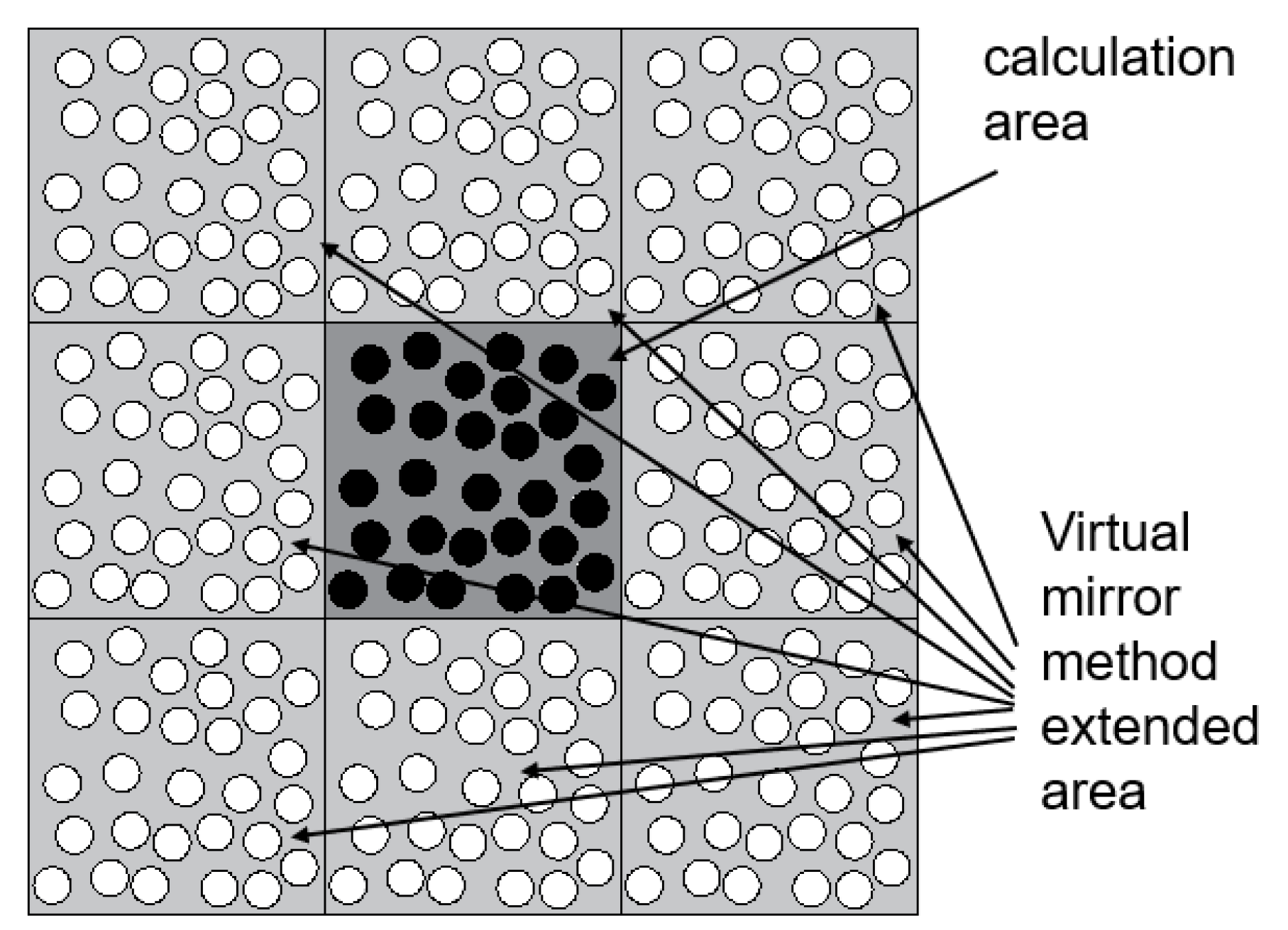
At the same time, in the process of computer simulation calculation, simulation can only be carried out in a limited area; the calculation area cannot be infinite, and its system has significant boundary limitations. In a limited area, particles will touch the system’s boundary and try to escape from the simulation area, which gradually increases the number of particles on the boundary. However, only a tiny portion of the particles exists on the boundary. This phenomenon is called the surface effect. To simulate the movement of natural fluids and create a virtual infinite calculation area, this topic uses virtual mirroring and rebound solid wall boundary conditions to eliminate the influence of surface effects in DPD simulation.
The virtual mirroring method refers to the realization of an approximately infinite calculation area by mirroring the distribution of coarse beads in the calculation domain to the position of the neighbourhood of the calculation domain. At the same time, the purpose of reducing the amount of calculation is realized, as shown in Figure 1.
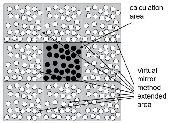
Figure 1.
Virtual mirror method.
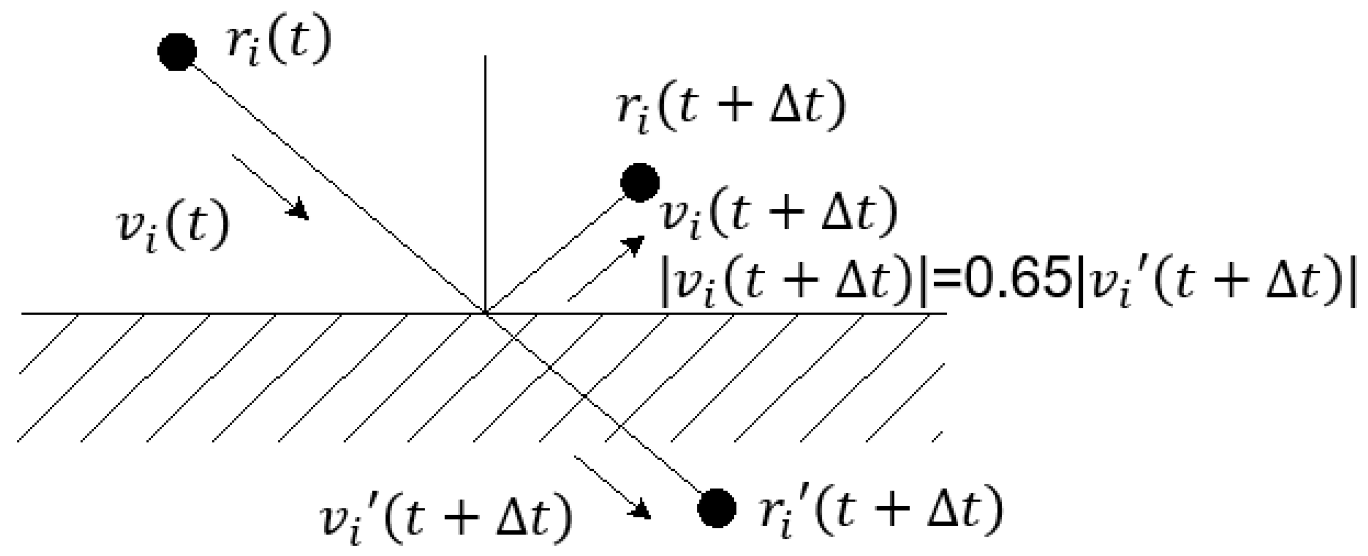
By “freezing” the particles, Revenga et al. [30] used the boundary fluid particles in a part of the calculation area as solid-wall particles. At present, many studies involving solid walls have adopted this boundary condition. The “frozen” solid wall particles not only cannot move, but also have the same flow characteristics as ordinary particles and can generate force like other particles. In addition, since, in the DPD system, the conservative force between particles is “soft”, the solid-walled particles cannot prevent the internal particles from crossing. This topic uses the Maxwellian rebound method to bounce the particles back to the calculation area. The fluid particle velocity obtained by the Maxwellian rebound method obeys the Maxwellian rebound distribution centred on the wall velocity, and when the thermal disturbance of the system is relatively large, the particle motion slips on the boundary. In this subject, the speed after slipping is simplified to 65% of the original speed, as shown in Figure 2.

Figure 2.
Maxwellian rebound method.
3. Simulation Condition
3.1. Physical Model and Validity Verification
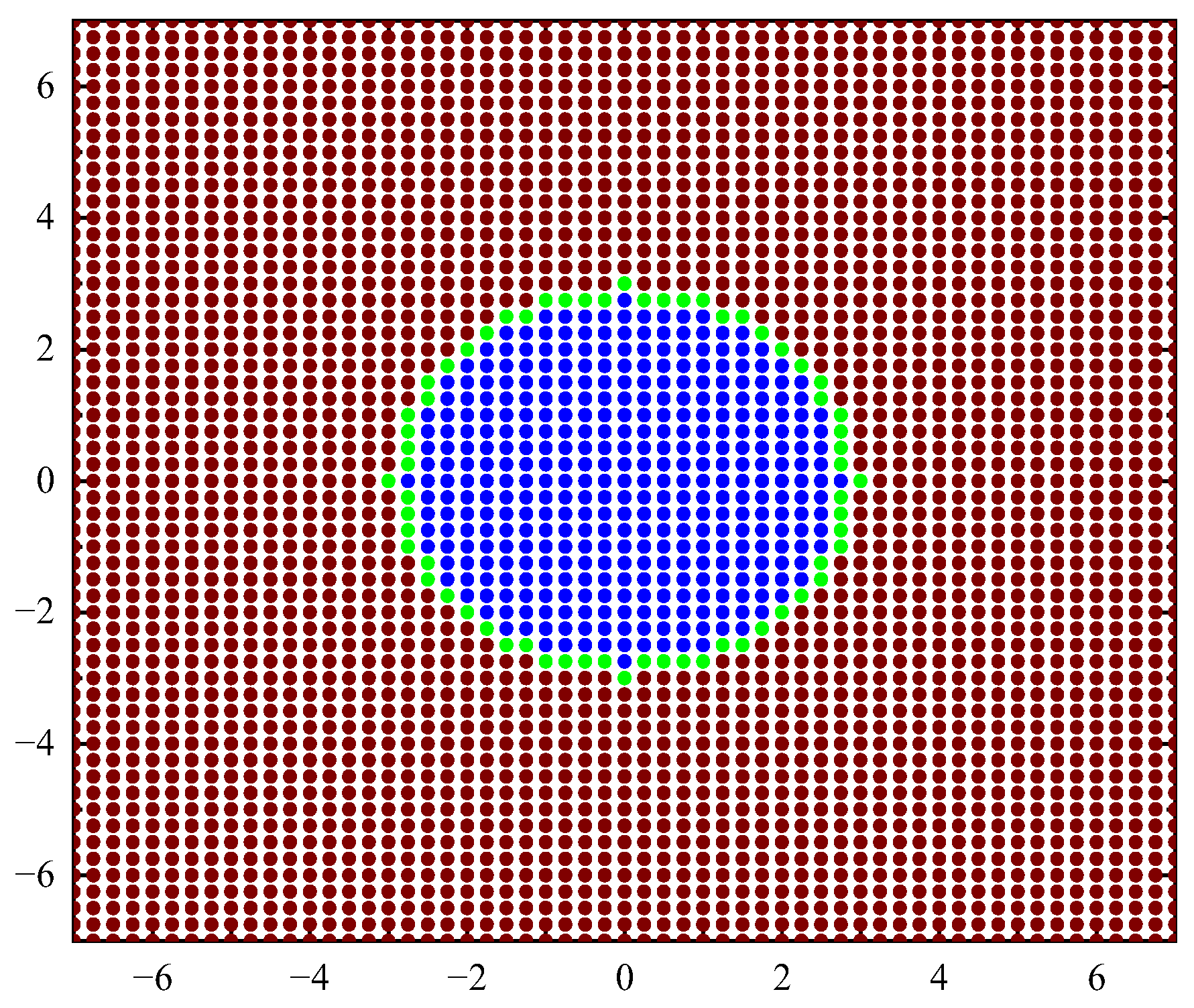
The geometric model is shown in Figure 3, and the fluid calculation domain is 14rc × 14rc. rc is the range of action of coarse beads or the cut-off radius, and its size changes accordingly with the size of the emulsion droplets. Based on the calculation model, the coarse beads are classified according to the type and force of the coarse beads. There are three types: continuous-phase (oil-phase) coarse beads, discrete-phase (water-phase) surface coarse beads that are polarized to generate polarization charges, and discrete-phase (water-phase) internal coarse beads.
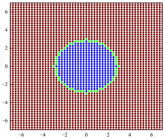
Figure 3.
Schematic diagram of physical model.
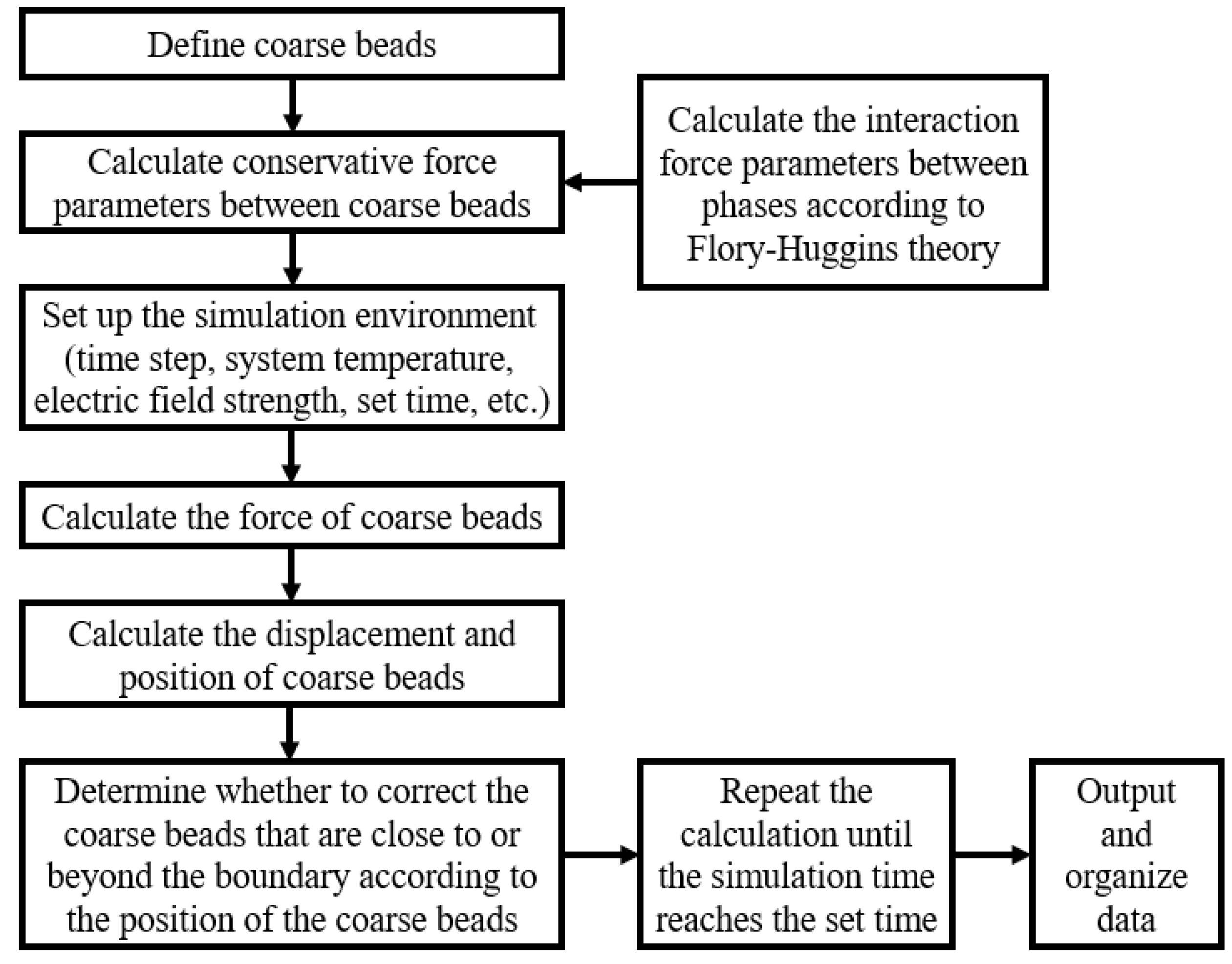
The conservative force parameters of the oil–water two-phase were first calculated using molecular simulation software, and then the force and deformation movement process of the emulsion droplets were analysed using Matlab programming (9.14.0.2206163, R2023a). The specific calculation steps are shown in Figure 4.
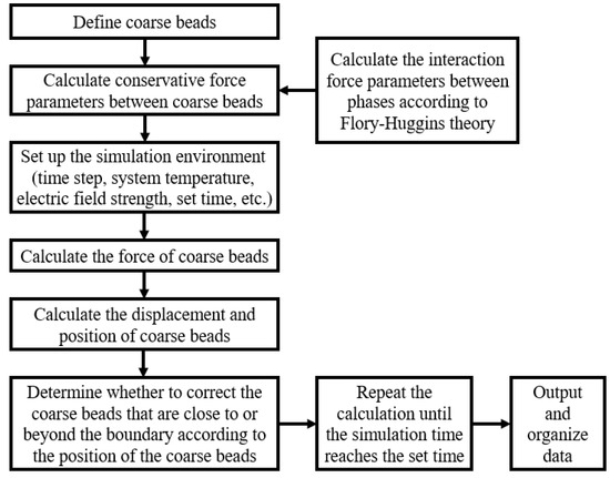
Figure 4.
Schematic diagram of calculation steps.
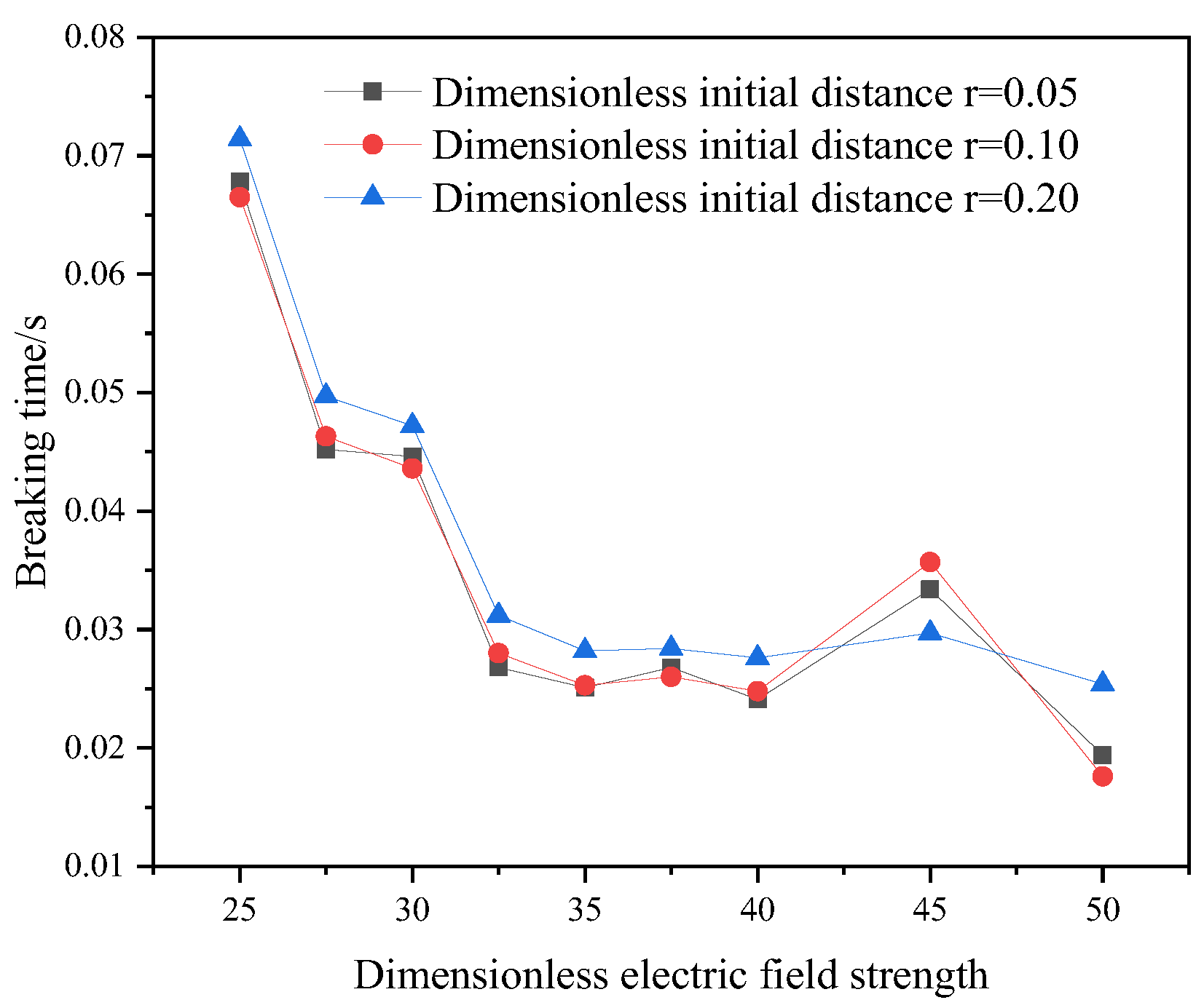
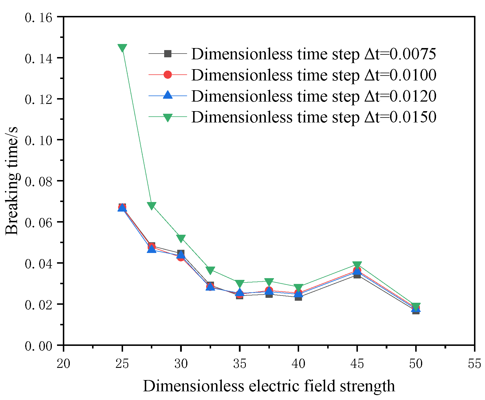
For the current physical model, a reasonable initial particle spacing and an appropriate spatial step size are conducive to saving calculation time and improving calculation accuracy. Based on three dimensionless initial particle spacings and four dimensionless time steps, the model’s breaking time under the action of the electric field is compared, and the results are shown in Figure 5 and Figure 6. When the dimensionless initial particle spacing is 0.1 and the dimensionless time step is equal to 0.01, the calculation result is stable. Therefore, the dimensionless initial particle spacing is selected as 0.1, and the dimensionless time step is 0.01.
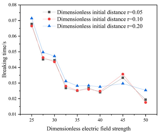
Figure 5.
Initial dimensionless coarse bead spacing verification.

Figure 6.
Dimensionless time step verification.
In order to verify the effectiveness of the simulation method, this work simulates the deformation process of the emulsion droplets under a weak electric field and compares the simulation results with the experimental results of Bin Li et al. [31]. In the model validation, the experimental and simulation conditions were the same, as follows: electric field strength E = 533 V mm−1; droplet size D = 1.196 and 2.800 mm; electric field types: sinusoidal, rectangular, and sawtooth; and interfacial tension of 0.025 N m−1. Deionized water was used as the dispersed phase, and sunflower oil was used as the continuous phase. The experimental and simulation results are shown in Figure 7, and the relative error expression is , where DRe and DRs are the experimental and simulation results of droplet deformation degree, respectively. It can be seen that the simulation results are in good agreement with the experimental results, and the maximum error does not exceed 18%.
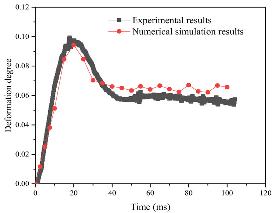
Figure 7.
Model validity verification.
3.2. Boundary Conditions and Simulation Settings
This work analyses various factors that affect emulsion droplets’ breaking and deformation behaviour under an electric field. Influencing factors include system temperature, oil phase type, oil phase conductive ion content, electric field strength, electric field frequency, and emulsion droplet size. The parameters used in the simulation are listed in Table 1.

Table 1.
The main parameters of the calculation.
4. Results and Discussion
4.1. The Deformation and Fragmentation Process of the Emulsion Droplet
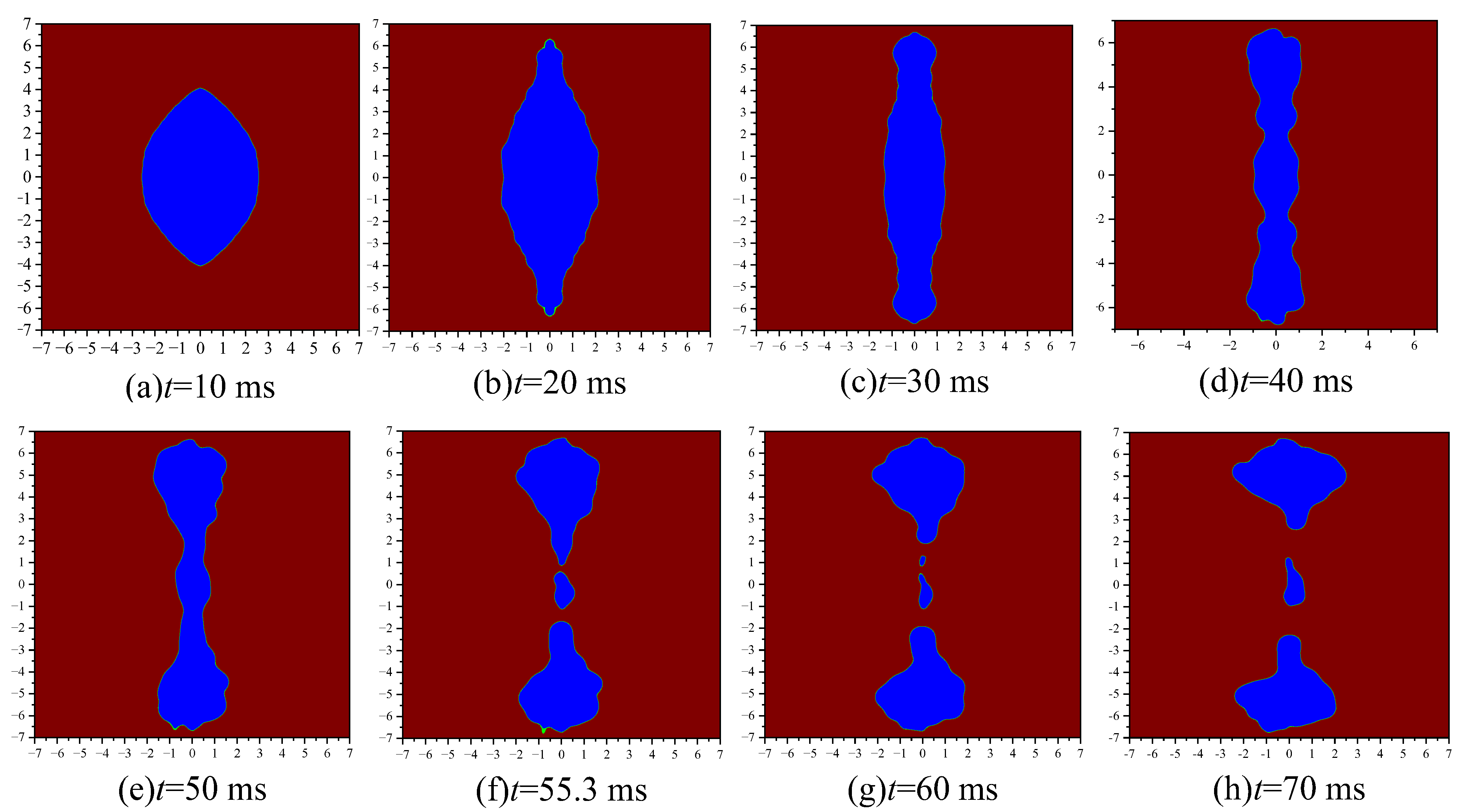
According to Figure 8, the emulsion droplets under the action of the electric field are divided into three stages. They are: (1) The charged coarse beads move under the electrostatic force of the electric field, and the emulsion droplets are stretched and deformed into long strips, as shown in Figure 8a–c. (2) During the emulsion droplet deformation process, the density of the coarse beads becomes smaller, forming some depressions, as shown in Figure 8d,e. (3) At the recessed position of the emulsion droplet, the droplet is squeezed and deformed by conservative forces, and then ruptures, as shown in Figure 8f–h.
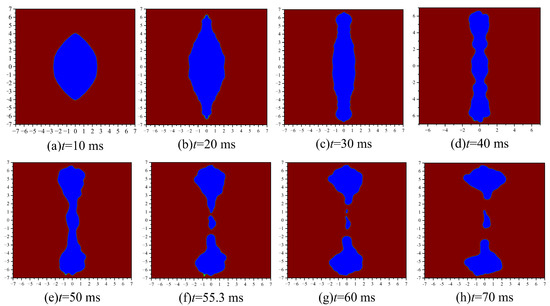
Figure 8.
Deformation and fragmentation process of emulsion droplets.
4.2. The Modification of the Agglomeration Kernel Function
Studies have shown that three main factors affect the deformation and breaking behaviour of emulsion droplets under the action of an electric field: the physical properties of oil and water, the external electric field, and the size of the emulsion droplets.
According to the idea of the DPD method, the oil–water properties of the deformation and breaking behaviour of emulsion droplets under the electric field mainly include the type of oil phase, the salt concentration in the oil phase, and the system temperature. In this study, molecular simulations were performed to calculate the solubility parameters of different oil phases and then to calculate different conservative force parameters to analyse the influence of oil phase types on emulsion droplets’ deformation and breaking behaviour under the electric field. The concentration of salts in the oil phase mainly affects the relative permittivity of the oil phase, thereby affecting the polarization charge of the coarse beads on the surface of the emulsion droplets. The influence of the system temperature in DPD is more complicated. On the one hand, the temperature increase will affect the solubility parameters of oil and water components obtained by molecular simulation and the conservative force parameters.
On the other hand, temperature increases will aggravate molecular irregularities. Thermal movement increases the random force intensity of the system. Therefore, to analyse the influence of the system temperature on the deformation and breaking behaviour of emulsion droplets, it is necessary to comprehensively consider the influence of the oil-phase conservative force coefficient and the random force intensity of the system. This study analyses the influence of the oil phase’s conservative force coefficient, the system random force strength, and the oil phase’s relative permittivity.
The influence of the electric field on the deformation and breaking behaviour of emulsion droplets is analysed. The electric field is mainly a sinusoidal alternating current, and the influence of the amplitude and frequency of the alternating current on emulsion droplets’ deformation and breaking behaviour is analysed. Due to the high frequency, the original time step cannot fully calculate the motion details in a single cycle for high-frequency sinusoidal alternating currents. Therefore, when analysing the influence of an electric field frequency greater than or equal to 1000 hz, this research carries out corresponding decreasing time steps so that the time step in each cycle is not less than 200.
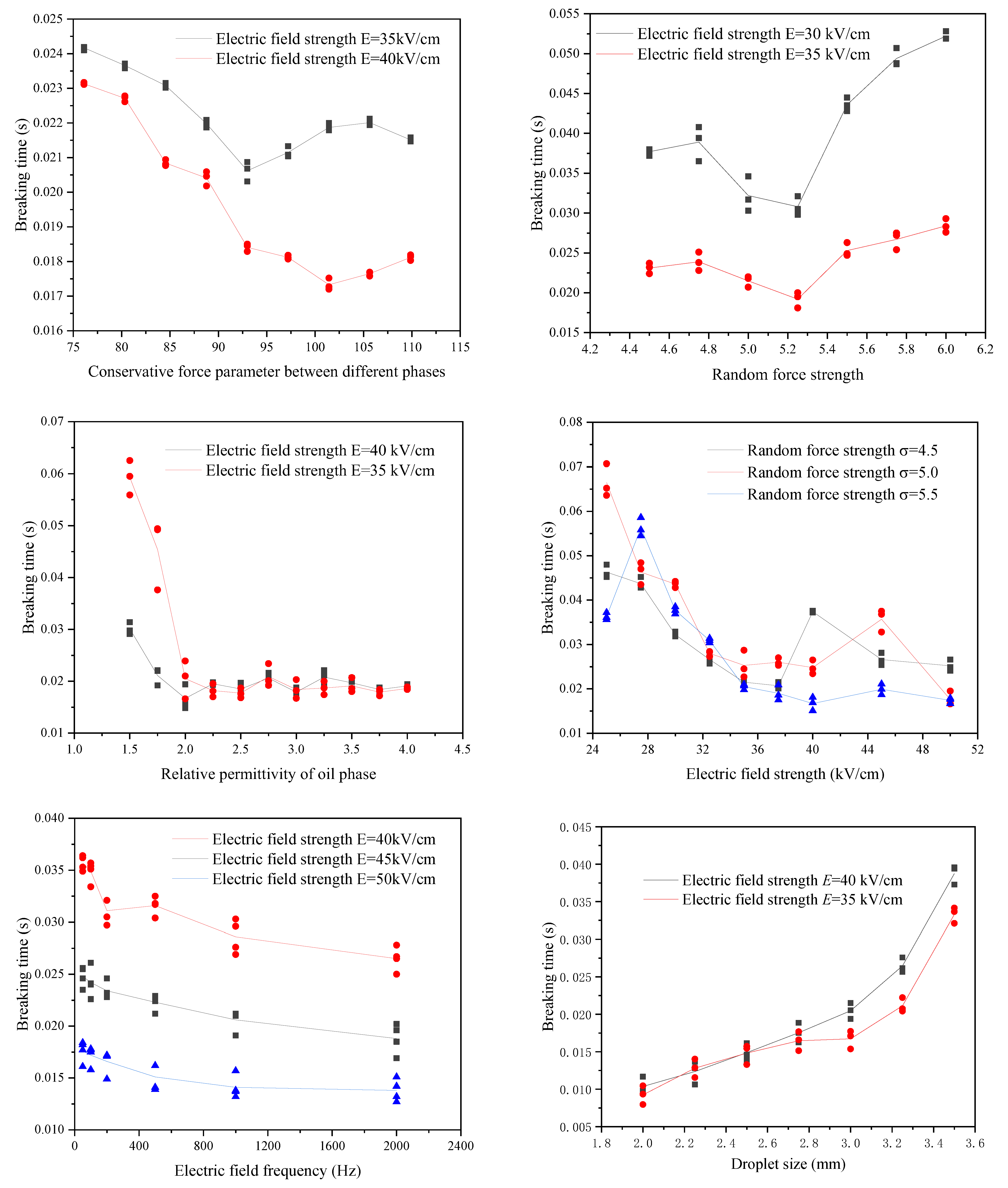
With the conservative force parameter increases between the different phases, the breaking time of the emulsion droplets under the electric field decreases first and then increases as shown in Figure 9. This is because the conservative force between the different phases mainly plays two roles: one is to maintain the existing shape during the stretching and deformation process of the emulsion droplets and hinder the deformation of the emulsion droplets; the other is to squeeze the emulsion droplets during the crushing stage to accelerate their breakup. When the conservative force parameter between the different phases is small, increasing the conservative force between the different phases will accelerate the squeezing of the emulsion droplets and cause them to break in a shorter time. When the conservative force parameter between the different phases is increased to a certain degree, it will hinder the emulsion droplets from stretching and deforming. The breaking time will increase accordingly. The same trend also occurs on the curve of random force intensity versus breaking time as shown in Figure 9. Since there is a specific equation relationship between the strength of random force and the strength of dissipative force, both must be analysed simultaneously. Increasing the strength of the random force and dissipation force will cause the viscosity and interfacial tension of the emulsion droplets to decrease, so it will accelerate the emulsion droplets’ deformation and promote the emulsion droplets’ breakage. However, excessive random force strength and dissipative force strength will neutralize the effect of a part of the conservative force and slow down the process of squeezing and breaking the emulsion droplets by the conservative force. The relative permittivity of the oil phase represents the polarization properties of the oil phase. The calculation method in this study assumes that the relative permittivity of the dispersed phase water is much greater than that of the continuous phase. The increase in the relative permittivity of the continuous phase (oil phase) within this range will increase the surface polarization charge of the emulsion droplets, thereby reducing the breaking time. However, as the relative permittivity of the oil phase increases, according to Equation (13), the increase in the surface polarization charge of the emulsion droplets continues to decrease. The increase rate of the oil phase’s relative permittivity decreases with the oil phase’s relative permittivity and gradually tends to a specific value.
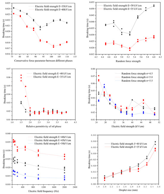
Figure 9.
The influence of various factors on the breaking behaviour of the emulsion under electric field.
The electric field strength of the electric field will determine the breaking time of the emulsion droplets, and the increase in the electric field’s electric field strength will promote the emulsion droplets’ deformation, thereby reducing the breaking time of the emulsion droplets as shown in Figure 9. However, when the electric field intensity increases to a particular value, the broken form of the emulsion droplets will change, which may lead to an increase in the breaking time and one or more peaks. However, when the electric field intensity exceeds this peak and continues to increase, the breaking time of the emulsion droplets will continue to decrease. When the electric field is a sinusoidal alternating current, increasing the frequency of the electric field will aggravate the vibration of the emulsion droplets’ deformation and reduce the emulsion droplets’ breaking time. The degree of increasing the frequency of the electric field to reduce the breaking time of emulsion droplets will gradually decrease with the frequency of the electric field.
As the size of the emulsion droplets increases, although the total polarized charge at the interface position of the emulsion droplets increases, the stretch deformation phenomenon is more likely to occur; however, due to the change in breaking form and the fact that the breaking process of emulsion droplets requires more conservative force to squeeze, the breaking time also increases.
4.3. Determination of Critical Electric Field Strength
In this study, the influence of various factors on the breaking behaviour of emulsion droplets under an electric field guides the actual production to promote or avoid breaking. Therefore, it is necessary to find the critical electric field strength of the emulsion droplets. When the electric field strength of the electric field is less than the critical electric field strength, only deformation and coalescence will occur, but no breaking will occur; when the electric field strength of the electric field is greater than the critical electric field, the droplets will be broken after a period of deformation.
The critical electric field strength of the emulsion droplets under a steady-current electric field is proportional to negative one-half of the droplet size, as shown in Equation (18). Due to the limitations of the DPD method itself, it is unable to fully describe the details of the molecular motion in the droplet. At the same time, the DPD method calculates the critical electric field strength, which can only guarantee that the droplet will deform and not break within the set time, and the droplets may still be broken outside the calculation time. In summary, two correction coefficients, A and B, are added to the critical electric field strength of the emulsion droplets under a steady-current electric field. A is the broken parameter after correction of the limitations of the DPD method, and B is the critical electric field intensity error due to the limitation of the simulation time, as shown in Equation (19):
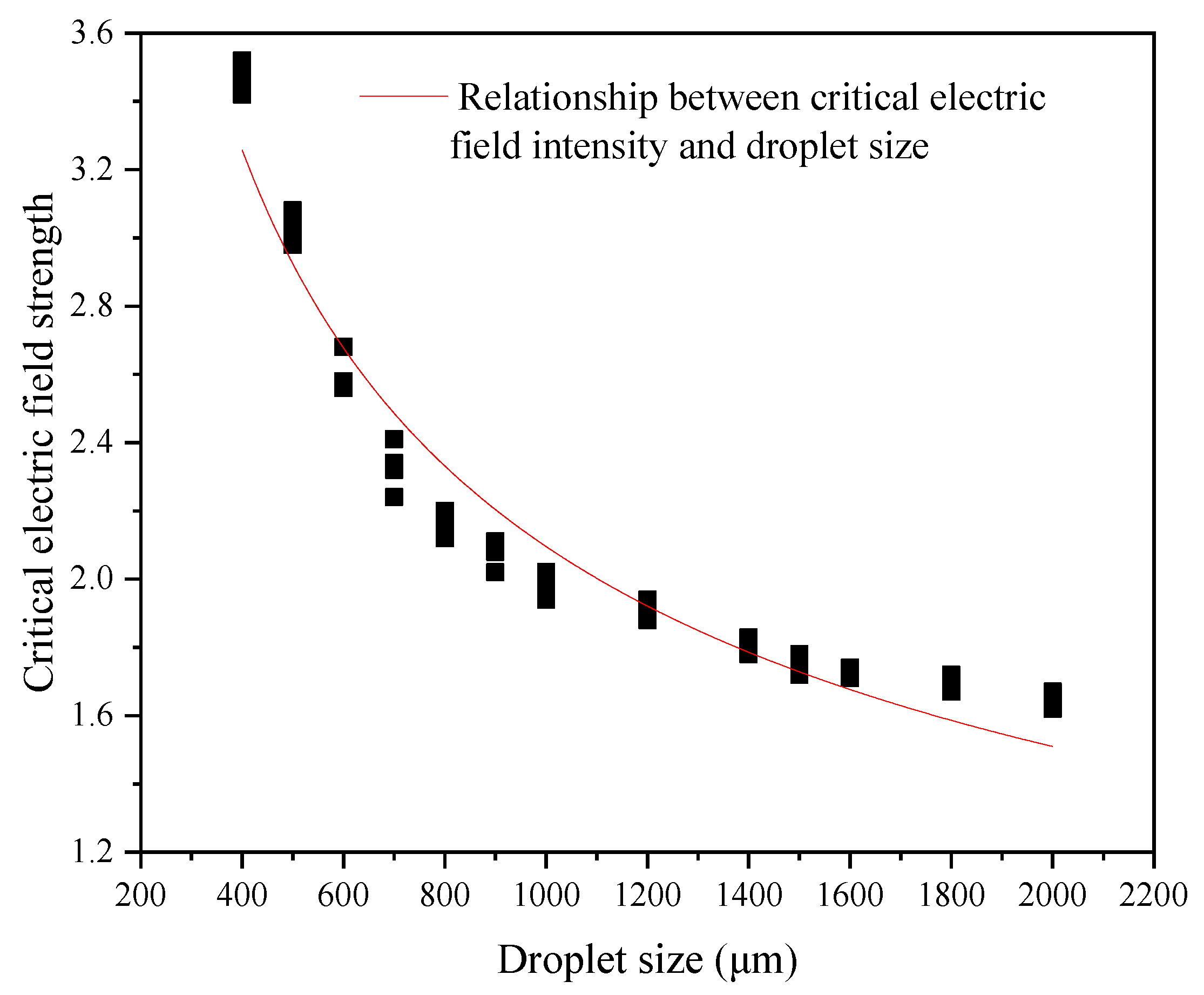
Figure 10 is a curve of the variation in the critical electric field intensity of the emulsion droplets with the size of the emulsion droplets obtained by numerical simulation. It can be seen that the critical electric field strength of the emulsion droplets and the size of the emulsion droplets are approximately one-half power. At the same time, due to the limitations of the DPD method and the simplified calculation process processing, there are specific errors between the numerical simulation results and the theoretical results.
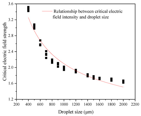
Figure 10.
Relationship between critical electric field intensity and droplet size.
The relationship curve between critical electric field intensity and droplet size is as follows:
5. Conclusions
This work uses the dissipative particle dynamics method to study the breaking and deformation process of fine emulsion droplets under a high-strength electric field, simplifying the calculation and ensuring calculation accuracy. In addition, various factors influencing the breaking time of emulsion droplets in the electric field are studied. Then, the critical electric field strength of the emulsion droplets is calculated, and the fitting curve of the critical electric field strength and the droplet size is obtained. It is summarized as follows:
- (1)
- The breaking process of emulsion droplets under the action of an electric field is divided into three stages: firstly, polarized charges are generated on the surface of the emulsion droplets and the emulsion droplets are stretched and deformed under the action of an electric field; secondly, during the stretching and deformation stage, as the particles inside the droplet move, the density of the droplet portion decreases, resulting in a particular area of depression; finally, the concave position is squeezed by conservative force to break the emulsion droplets.
- (2)
- The physical properties of oil and water, the electric field, and the size of the emulsion droplets significantly affect the breaking time of emulsion droplets. For example, as the conservative force parameter and the random force intensity increase, the breaking of emulsion droplets first speeds up and then slows down; the breaking time decreases with the increase in the relative permittivity of the oil phase and the amplitude and frequency of the electric field; as the droplet size increases, the breaking time also increases.
- (3)
- The critical electric field strength of the emulsion droplets was calculated. The results show that the critical electric field strength of the emulsion droplets and the size of the emulsion droplets were approximately minus one-half power, and due to the limitations of the DPD method and the simplified processing of the calculation process, specific corrections were made when fitting the numerical simulation results. The fitting relationship is as in Equation (20).
Author Contributions
Conceptualization, W.X.; Methodology, W.X.; Validation, Y.G.; Formal analysis, C.L.; Data curation, W.X.; Writing—original draft, W.X.; Writing—review & editing, X.Y.; Visualization, Y.G. All authors have read and agreed to the published version of the manuscript.
Funding
This research received no external funding.
Data Availability Statement
The original contributions presented in the study are included in the article, further inquiries can be directed to the corresponding author.
Conflicts of Interest
Author Lv, C. was employed by the company China Petroleum Pipeline Bureau Engineering Co., Ltd., Third Engineering Branch. The remaining authors declare that the research was conducted in the absence of any commercial or financial relationships that could be construed as a potential conflict of interest.
References
- Bailes, P.J. An experimental investigation into the use of high voltage DC fields for liquid phase separation. Trans. Inst. Chem. Eng. 1981, 59, 229–237. [Google Scholar]
- Alves, R.P.; Oliveira, R.C. Petrobras. How to establish a mathematical model for the electroststic desalting process based on pilot plant studies. In Proceedings of the the SPE Annual Technical Conference and Exhibition, San Antonio, TX, USA, 24–27 September 2006; pp. 1–5. [Google Scholar]
- Lu, G.; Lu, Q.H.; Li, P.S. Break-down of liquid membrane emulsion under high electric field. J. Membr. Sci. 1997, 128, 1–6. [Google Scholar]
- Tsuneki, I.; Keisuke, I.; Shigeki, Y.; Masao, S. Rapid demulsification of dense oil-in-water emulsion by low external electric field I. Experimental evidence. Colloids Surf. A Physicochem. Eng. 2004, 242, 21–26. [Google Scholar]
- Taylor, S.E. Investigations into the electrical and coalescence behaviour of water-in-crude oil emulsions in high voltage gradients. Colloids Surf. 1988, 29, 29–51. [Google Scholar] [CrossRef]
- Yong, M.J.; Hyun, C.O. Electrical charging of a conducting water droplet in a dielectric fluid on the electrode surface. J. Colloid Interface Sci. 2008, 322, 617–623. [Google Scholar]
- Noik, C.; Chen, J.Q.; Dalmazzone, C. Electrostatic Demulsification on Crude Oil: A State-of-the-Art Review. In Proceedings of the the International Oil & Gas Conference and Exhibition in China, Beijing, China, 5–7 December 2006; pp. 1–12. [Google Scholar]
- John, S.E.; Mojtaba, G. Electrostatic enhancement of coalescence of water droplets in oil: A review of the current understanding. Chem. Eng. J. 2001, 85, 173–192. [Google Scholar]
- Waterman, L.C. Electrical coalesces. Chem. Eng. Prog. 1965, 61, 51–57. [Google Scholar]
- Merv, F. Water-in-Oil Emulsion Formation: A Review of Physics and Mathematical Modelling. Spill Sci. Technol. Bull. 1995, 2, 55–59. [Google Scholar]
- Der, O.; Bertola, V. An experimental investigation of oil-water flow in a serpentine channel. Int. J. Multiph. Flow 2020, 129, 103327. [Google Scholar] [CrossRef]
- Sarkar, P.S.; Singh, K.K.; Shenoy, K.T.; Sinha, A.; Rao, H.; Ghosh, S.K. Liquid–Liquid Two-Phase Flow Patterns in a Serpentine Microchannel. Ind. Eng. Chem. Res. 2012, 51, 5056–5066. [Google Scholar] [CrossRef]
- Taylor, G. Studies in electrohydrodynamics. I. The circulation produced in a drop by an electric field. Proc. R. Soc. Lond. 1966, 291, 159–166. [Google Scholar]
- Torza, S.; Cox, R.G.; Mason, S.G. Electrohydrodynamic deformation and burst of liquid drops. Phil. Traps. R. Soc. Lond. 1971, 269, 295–319. [Google Scholar]
- Ajayi, O.O. A note on Taylor’s electrohydrodynamic theory. Proc Roy Soc. Lond. A 1978, 364, 499–507. [Google Scholar]
- Hua, L.; Lirn, L.K.; Wang, C.H. Numerical simulation of deformation/motion of a drop suspended in viscous liquids under influence of steady electric fields. Phys. Fluids 2008, 20, 113302. [Google Scholar] [CrossRef]
- Tomar, G.; Gerlach, D.; Biswas, G.; Alleborn, N.; Sharma, A.; Durst, F.; Welch, S.W.J.; Welch, A. Two-phase electrohydrodynamic simulations using a volume-of-fluid approach. Comput. Phys. 2007, 227, 1267–1285. [Google Scholar] [CrossRef]
- Sonic, P.; Juvekar, V.A.; Naik, V.M. Investigation on dynamics of double emulsion droplet in a uniform electric field. J. Electrost. 2013, 71, 471–477. [Google Scholar] [CrossRef]
- Eow, J.S.; Ghadiri, M. Drop-drop coalescence in an electric field: The effects of applied electric field and electrode geometry. Colloids Surfaces A Physicochem. Eng. 2003, 219, 253–279. [Google Scholar] [CrossRef]
- Eow, J.S.; Ghadiri, M.; Sharif, A. Experimental studies of deformation and break-up of aqueous drops in high electric fields. Colloids Surfaces A Physicochem. Eng. 2003, 225, 193–210. [Google Scholar] [CrossRef]
- Eow, J.S.; Ghadiri, M.; Sharif, A. Deformation and break-up of aqueous drops in dielectric liquids in high electric fields. J. Electrost. 2001, 51, 463–469. [Google Scholar] [CrossRef]
- Lac, E.; Homsy, G.M. Axisymmetric deformation and stability of a viscous drop in a steady electric field. J. Fluid Mech. 2007, 590, 239264. [Google Scholar] [CrossRef]
- Ha, J.; Yang, S. Effects of surfactant on the deformation and stability of a drop in a viscous fluid in an electric field. Colloid Interface Sci. 1995, 175, 369–385. [Google Scholar] [CrossRef]
- Ha, J.; Yang, S. Effect of nonionic surfactant on the deformation and breakup of a drop in an electric field. Colloid Interface Sci. 1998, 206, 195–204. [Google Scholar] [CrossRef] [PubMed]
- Hoogerbrugge, P.J.; Koelman, J.M.V.A. Simulating microscopic hydro-dynamic phenomena with dissipative particle dynamics. Euro Phys. Lett. 1992, 19, 155–160. [Google Scholar] [CrossRef]
- Espańol, P.; Warren, P. Statistical mechanics of dissipative particle dynamics. Lett. Euro Phys. 1995, 30, 191–196. [Google Scholar] [CrossRef]
- Groot, R.D.; Warren, P.B. Dissipative particle dynamics: Bridging the gap between atomistic and mesoscopic simulation. Chem. Phys. 1997, 107, 4423. [Google Scholar] [CrossRef]
- Liyana-Arachchi, T.P.; Jamadagni, S.N.; Eike, D.; Koenig, P.H.; Siepmann, J.I. Liquid-liquid equilibria for soft-repulsive particles: Improved equation of state and methodology for representing molecules of different sizes and chemistry in dissipative particle dynamics. Chem. Phys. 2015, 142, 044902. [Google Scholar] [CrossRef] [PubMed]
- Español, P.; Warren, P.B. Perspective: Dissipative particle dynamics. Chem. Phys. 2017, 146, 150901. [Google Scholar] [CrossRef] [PubMed]
- Revenga, M.; Zuniga, I.; Espanol, P. Boundary model in DPD. Int. J. Mod. Phys. C 1998, 9, 1319–1328. [Google Scholar] [CrossRef]
- Li, B.; Vivacqua, V.; Ghadiri, M.; Sun, Z.; Wang, Z.; Li, X. Droplet deformation under pulsatile electric fields. Chem. Eng. Res. Des. 2017, 127, 180–188. [Google Scholar] [CrossRef]

Disclaimer/Publisher’s Note: The statements, opinions and data contained in all publications are solely those of the individual author(s) and contributor(s) and not of MDPI and/or the editor(s). MDPI and/or the editor(s) disclaim responsibility for any injury to people or property resulting from any ideas, methods, instructions or products referred to in the content. |
© 2024 by the authors. Licensee MDPI, Basel, Switzerland. This article is an open access article distributed under the terms and conditions of the Creative Commons Attribution (CC BY) license (https://creativecommons.org/licenses/by/4.0/).