Vorticity and Its Relationship to Vortex Separation, Dynamic Stall, and Performance, in an H-Darrieus Vertical-Axis Wind Turbine Using CFD Simulations

Abstract

Vortices play a critical role in the operation of VAWTs (Vertical-Axis Wind Turbines). In spite of this, most studies have approached these matters via the qualitative analysis of vortex shedding, and torque-extraction data. These approaches rely only on the visual observation of vortices that can lead to subjective interpretations. In our work, a 3D framework is employed to address this issue. On this basis, the present study establishes a relationship between vorticity, dynamic stall and turbine performance, by examining various locations along the span and the chord of the airfoil. To conduct this analysis, a 3D-CFD (Computational Fluid Dynamics) simulation of an H-Darrieus with a symmetrical NACA 0018, powered by 8 m/s winds, is considered. The CFD simulations are validated based on the agreement of calculated power coefficients, with those obtained from experimental data, reported in the technical literature, with deviations being lower than 4%. The simulation results for various TSRs (Tip Speed Ratios) report new findings concerning the critical stages of VAWT operation. This shows that there is a link between the maximum vorticity, the imminent vortex-separation condition and the dynamic stall, with this being a function of the various axial positions in the VAWT.

1. Introduction

The growing global commitment to sustainable energies has led to a remarkable rise in the adoption of renewable energy sources, given that they are clean, inexhaustible, and increasingly competitive. On the world scale, more than 80% of the energy requirements are obtained via the consumption of fossil fuels [1,2]. Thus, there is still a significant need to enhance existing technologies and/or to create new ones in order to achieve a successful transition towards renewable and sustainable energies.

In particular, wind has become a valuable source of renewable energy due to its cost-effectiveness when harvesting energy with turbines, and in particular when integrated with other alternative energy sources such as solar, which relies on photovoltaic panels [3,4]. Wind also offers a unique opportunity to be combined with hydrogen production, which has gained great interest due to its wide applications such as replacing conventional portable batteries, vehicle fuels, and home energy needs [5]. This can be achieved by incorporating hybrid technology, where wind turbines are used to generate electricity that can be used later to produce hydrogen via electrolysis or photocatalysis [6].

Wind turbines are used to convert the kinetic energy of the wind into mechanical energy, which can be used to generate electricity [7]. There are two basic types of wind turbines: (i) Horizontal Axis Wind Turbines (HAWTs) and (ii) Vertical-Axis Wind Turbines (VAWTs). HAWTs are more widely used due to their claimed higher efficiency compared to VAWTs [8]. However, HAWTs have drawbacks, such as the high cost of maintenance, specific location requirements, wind direction dependency, and wind speed limitations. On the other hand, VAWTs operate independently of wind direction, given that the power generation equipment is compact, and can be located at ground level, which makes their maintenance easier [9,10].

VAWTs are subjected to complex flow patterns and aerodynamic phenomena, such as dynamic stall, which is a phenomenon that includes the formation, growth, and shedding of blade-scale vortices, followed by flow separation [11]. Thus, understanding vortices in VAWTs is crucial in order to enhance their aerodynamic efficiency, minimize energy losses, and improve overall VAWT performance. To accomplish this, several authors have studied vortices in VAWTs using CFD simulations, because it is a cost-effective and accurate tool to analyze unsteady aerodynamics [12,13,14,15,16].

The majority of CFD studies on Vertical-Axis Wind Turbines (VAWTs) have been conducted in 2D. For instance, a comprehensive review of 2D RANS CFD studies were reported in [17]. This article also provides insights into the numerical settings commonly employed in Darrieus rotor RANS studies, along with guidelines for the optimal configuration of these simulations. However, using 2D simulations to analyze the airflow patterns around rotors can introduce significant uncertainties. This is mainly due to the challenges in precisely measuring complex 3D aerodynamic features, like blade-tip flows, which could lead to an overestimation of energy extraction [18,19,20]. Moreover, the spatial variability of key 3D aerodynamic structures in Darrieus rotor flows increases this problem, particularly with the delayed formation of the tip vortex compared to the mid-blade vortex [13,17]. Thus, the use of 3D CFD simulations is essential for effectively modeling Vertical-Axis Wind Turbines (VAWTs).

As previously noted, a comprehensive understanding of vortices in Vertical-Axis Wind Turbines (VAWTs) is critical for optimizing their aerodynamic efficiency. This is apparent in a significant portion of studies that investigate VAWTs, whether they involve a standard examination of a specific design or an exploration of design parameter variations such as the angle of attack, the implementation of winglets, the airfoil profile and the aspect ratio. In such studies, there is a consistent analysis of vorticity contours in order to examine the vortex structure, offering valuable insights to enhance the structural performance of blades [21]. These analyses not only visualize the effects of vortex development but also contribute to improving blade performance.

Vorticity is a fundamental aerodynamic parameter for establishing VAWT performance. For instance, works by [22,23,24] delve deeply into this subject. One could argue for the utilization of the velocity field, instead. However, as noted by Kheradvar in [22], velocity alone fails to capture the intricate dynamical aspects of a flow field, such as stresses, mixing, or turbulence, which depend on velocity gradients. This limitation becomes especially pronounced in the presence of vortex structures within the fluid motion. Vorticity, on the other hand, provides a quantitative measure of fluid flow rotation around turbine blades. It offers crucial insights into the formation, interaction, and dissipation of vortices, having a significant impact on the extracted torque and on the overall efficiency of the turbines [22]. Vorticity provides a comprehensive description of the flow and facilitates the reconstruction of the entire velocity field.

Another critical aspect is that vorticity cannot spontaneously emerge within the fluid; it can only be created between the fluid and the boundaries (e.g., blade wall). Furthermore, vorticity can be transported by either diffusion or convection. Additionally, it is essential to clarify that a vortex is not solely characterized by circulatory motion; rather, it denotes a region where vorticity has accumulated. This feature is critical, as the circulatory pattern may sometimes remain covered behind an irrotational contribution that masks its rotational features [22].

Even if various authors in the literature [12,21,25,26,27] have envisioned the importance of vortices in the near airfoil region, as a main factor of turbine performance, there is still the need of a quantitative vorticity analysis that considers the azimuthal angular ranges which lead to the vortex conditions contributing to the largest torques. Recognizing this, in 2023, Acosta-Lopéz et al. [28] at CREC (Chemical Reactor Engineering Centre), UWO, proposed a way to carry out a quantitative vortex analysis. These authors introduced the definition of the Vorticity Index, where events such as the vortex imminent separation condition can be measured quantitatively and are untied to visual references [28]. Nevertheless, their study was conducted in a 2D space, and effects like tip vortices were not accounted for.

It is, in this respect, known that ignoring end-blade phenomena such as tip vortices, can lead to inaccurate results [18]. Thus, the use of 3D models is strongly recommended for vorticity analyses, as summarized in

Table 1. Comparison of 2D and 3D Models for Vertical-Axis Wind Turbines (VAWTs).

Aspect	2D	3D
Flow Field	Considers a uniform, two-dimensional flow across the vertical span of the rotor-blade flow field.	Accounts for the non-uniformity of the flow across the vertical span of the rotor by considering tip losses and other aspects of three-dimensionality such as vertical vortices.
Accuracy	Reasonable for simple VAWT designs and operating conditions. It can overpredict the Cp values at high TSR values (TSR > 1).	Higher for complex VAWT designs and operating conditions, especially when the flow is affected by turbulence at the tips, dynamic stall, and other non-linear phenomena.
Computational Cost	Less expensive than 3D simulations, as 2D models require fewer grid points and shorter computational times.	More expensive than 2D simulations, as 3D calculations require more grid points and larger computational times.
Limitations	Captures partially the flow phenomena such as vortex shedding, tip vortices, blade–wake interactions, and flow separation.	Capture the complex flow phenomena that occur in VAWTs using advanced modeling and major computational resources.
Applications	Suitable for preliminary design and calculations.	Suitable for detailed design and fluid-dynamic studies, with a focus on vorticity, and on the impact of design parameters on the VAWT performance and efficiency.

Note: TSR = Tip Speed Ratio, Cp = Power Coefficient, VAWT = Vertical-Axis Wind Turbine.

.

Therefore, to achieve a better description and understanding of the effects of the three-dimensional flow and vortex development on the overall performance of a VAWT, the present study analyses the following: (a) 3D flow simulations of an H-type Darrieus turbine operation, (b) quantitative vorticity evaluations including dynamic stall, and (c) local torque calculations to establish turbine performance.

2. Numerical Methodology

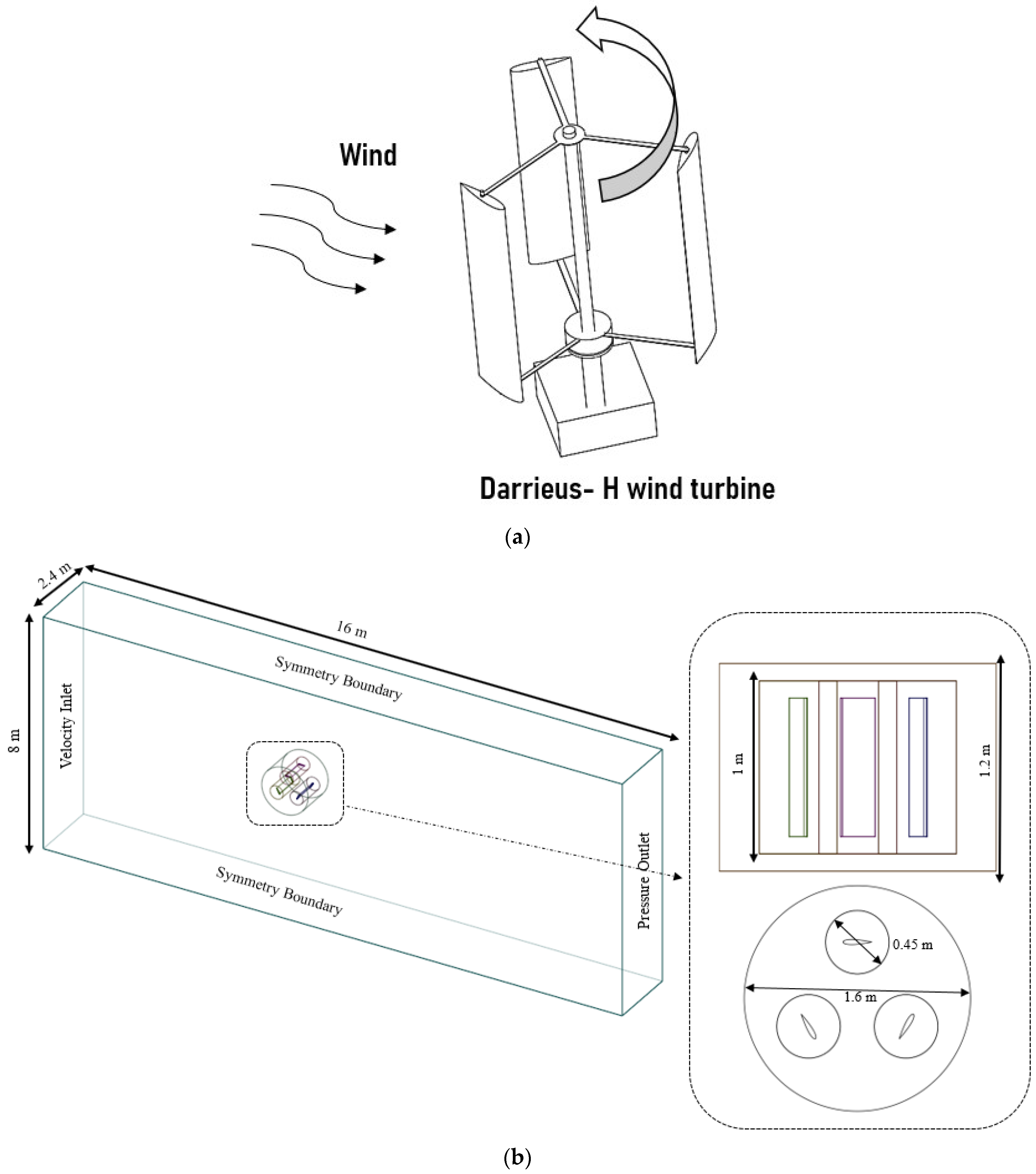
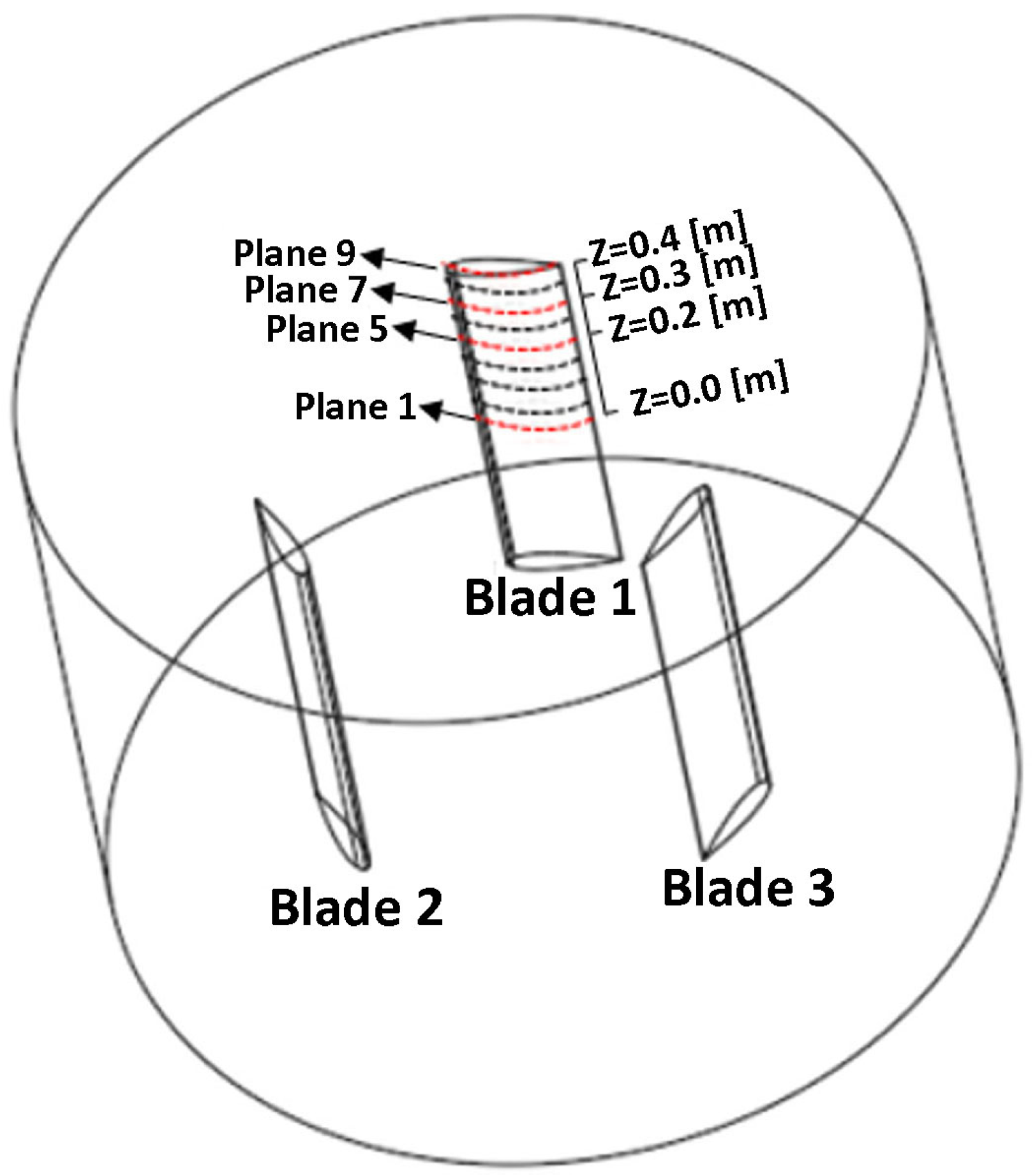
2.1. Physical Model

This study focuses on a three-blade H-Darrieus turbine with a NACA0018 blade configuration, as described in Figure 1a.

Regarding this turbine, the rotor’s dimension and the computational domains were taken from research conducted by Ma Ning et al. in 2018 [21], as reported in

Table 2. Design Parameters of the H-Darrieus Wind Turbine Studied [21].

Parameter	Symbol	Value
Rotor Diameter [m]	D	0.8
Blade Airfoil	-	NACA 0018
Chord Length [m]	c	0.2
Rotor Height [m]	H	0.8
Blade Number	N	3
Solidity	σ	0.75

Note: solidity, $\sigma =\frac{\mathrm{N}·\mathrm{c}}{\mathrm{D}}$

, with the shaft being omitted from the modeling analysis.

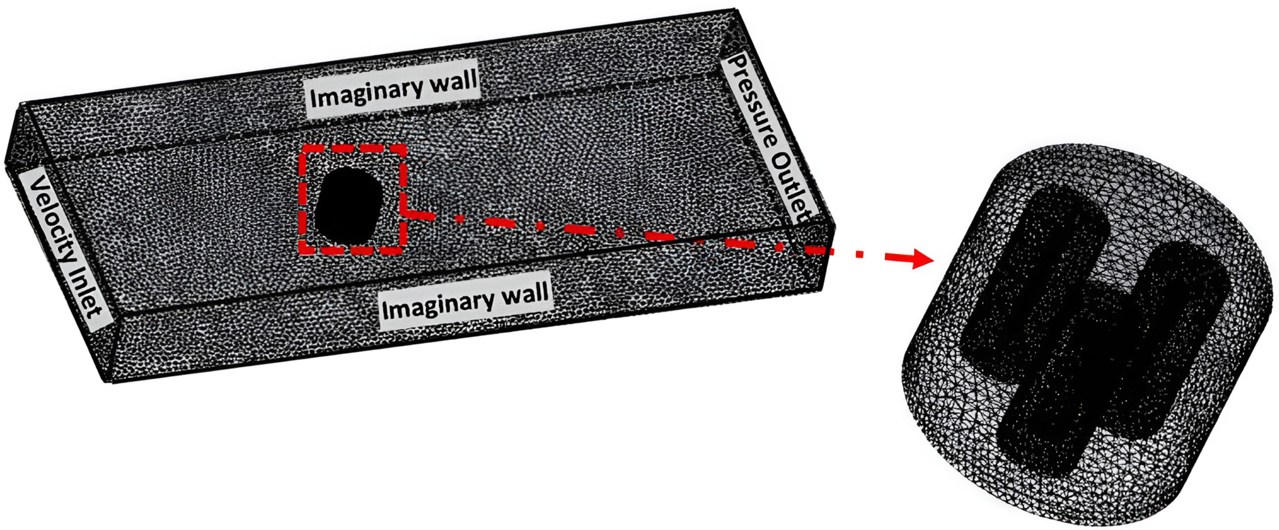
2.2. Computational Domains

CFD simulations for vertical-axis wind turbines, typically, involve five domains of interest: (i) a fixed domain that represents an imaginary hexahedron control volume, (ii) a rotating domain that accounts for the presence of the VAWT rotor, and (iii) three subdomains (one for each blade) that are utilized to guarantee a more refined mesh surrounding the blades. The computational domain dimensions employed were the ones proposed in [21]. This was carried out in order to have an adequate basis for numerical model validation.

Computational calculations consider an imaginary fixed domain, described in Figure 1b. These involved the following assumptions: (a) a constant inlet air velocity (${\mathrm{U}}_{\infty }$ = 8 m/s), (b) a fixed-domain exit flow, with a zero-exit gauge pressure, (c) a 1% air-flow turbulence, at the inlet fixed-domain condition, and (d) a fluid velocity, at the imaginary upper, lower and lateral boundaries, with this being the same as the incoming wind flow. In addition, a non-slip-wall state operating condition was assigned to the rotor blade surfaces. To connect the fixed and rotating domains, an interface boundary condition was assigned. Furthermore, by performing a sensitivity analysis based on grid size changes, it was ensured that the selected grid sizes for the domains near the interface were properly selected, facilitating, in this manner a smooth data exchange between calculation domainths during simulations.

2.3. Solver Setting

The commercial software ANSYS 21.1 Fluent was used for the CFD simulations. The following continuity (Equation (1)) and momentum balances (Equation (2)), using URANS (Unsteady Reynolds-Averaged Navier–Stokes), were considered as follows:

$${\displaystyle \frac{\partial }{\partial t}}·\rho +𝛻·(\rho \overrightarrow{u})=0$$

(1)

$${\displaystyle \frac{\partial }{\partial t}}\left(\rho \overrightarrow{u}\right)+𝛻·(\rho \overrightarrow{u}\overrightarrow{u})=-𝛻P+𝛻·\tau +\rho \overrightarrow{g}+\overrightarrow{F}$$

(2)

where P represents the static pressure, $𝛻$ is the divergence operator, $\overrightarrow{u}$ is the flow velocity, $\tau$ is the stress tensor, $\overrightarrow{\rho g}$ and $\overrightarrow{F}$ are the gravitational body force and external forces, respectively. The stress tensor ($\tau )$ was calculated, as shown in Equation (3), with $\mu$ being the molecular viscosity and I being the unit tensor. One should note that ${\left(𝛻\overrightarrow{u}\right)}^{\mathrm{T}}$ stands for the transpose of the divergence matrix (i.e., rate of expansion) of the flow [18,29].

$$\tau =\mu [(𝛻\overrightarrow{u}+{\left(𝛻\overrightarrow{u}\right)}^T)-{\displaystyle \frac{2}{3}}𝛻·\overrightarrow{u}I]$$

(3)

The CFD numerical model used to carry out these simulations using ANSYS 21.1 Fluent was the SST k-ω two equations turbulence model. This model belongs to the Reynolds-averaged Navier–Stokes (RANS) family of turbulence models. The SST k-ω model is widely used to conduct VAWTs simulations, due to its ability to predict pressure-induced separation, as well as the fluid viscous–inviscid interactions, making this model a good choice for aerodynamic applications [18,30].

As a result, the k turbulent-fluid kinetic energy and the $\omega$ specific turbulence dissipation rate can be considered via Equations (4) and (5), respectively, as follows:

$${\displaystyle \frac{\partial }{\partial t}}\left(\rho k\right)+{\displaystyle \frac{\partial }{\partial x_i}}\left(\rho k{u}_i\right)={\displaystyle \frac{\partial }{\partial x_j}}\left({\Gamma }_k{\displaystyle \frac{\partial k}{\partial x_j}}\right)+G_k-Y_k+S_k$$

(4)

$${\displaystyle \frac{\partial }{\partial t}}\left(\rho \omega \right)+{\displaystyle \frac{\partial }{\partial x_i}}\left(\rho \omega u_i\right)={\displaystyle \frac{\partial }{\partial x_j}}\left({\Gamma }_{\omega }{\displaystyle \frac{\partial \omega }{\partial x_j}}\right)+G_{\omega }-Y_{\omega }+S_{\omega }$$

(5)

with $G_k$ representing the turbulence kinetic-energy generation and $G_{\omega }$ standing for the generation of $\mathsf{\omega }$. Both variables are defined as in the standard k-ω model. ${\Gamma }_k$ and ${\Gamma }_{\omega }$ denote the effective diffusivities for both k an $\omega$, respectively. $Y_k$ and $Y_{\omega }$ represent k and $\mathsf{\omega }$ dissipations due to turbulence, respectively. $D_{\omega }$ stands for the cross-diffusion, and $S_k$ and $S_{\omega }$ represent the user-defined source terms.

Table 3. Numerical CFD Simulation Data.

Parameter	Symbol	Value
Viscous model	SST k-ω	k-ω Shear Stress Transport
Air density	$\rho$	1.225 kg/m3
Air viscosity	μ	1.79 × 10−5 Pa s
Air velocity	$\mathrm{U}$∞	8 m/s
Reynolds number	Re	1.09 × 105
Turbulent intensity		1%
Tip-speed ratio	λ	0.5–1.5
Solver type		Pressure-Based
Coupling Method		Coupled
Time discretization		2° of rotation per time-step
Residuals		1 × 10−4

Note: (a) tip-speed ratio,$\mathsf{\lambda }={\displaystyle \frac{\mathsf{\omega }·\mathrm{R}}{{\mathrm{U}}_{\infty }}}$ (b) incompressible fluid.

reports the values assigned to the various parameters involved in the turbine simulations, such as the fluid physical properties and the solver settings.

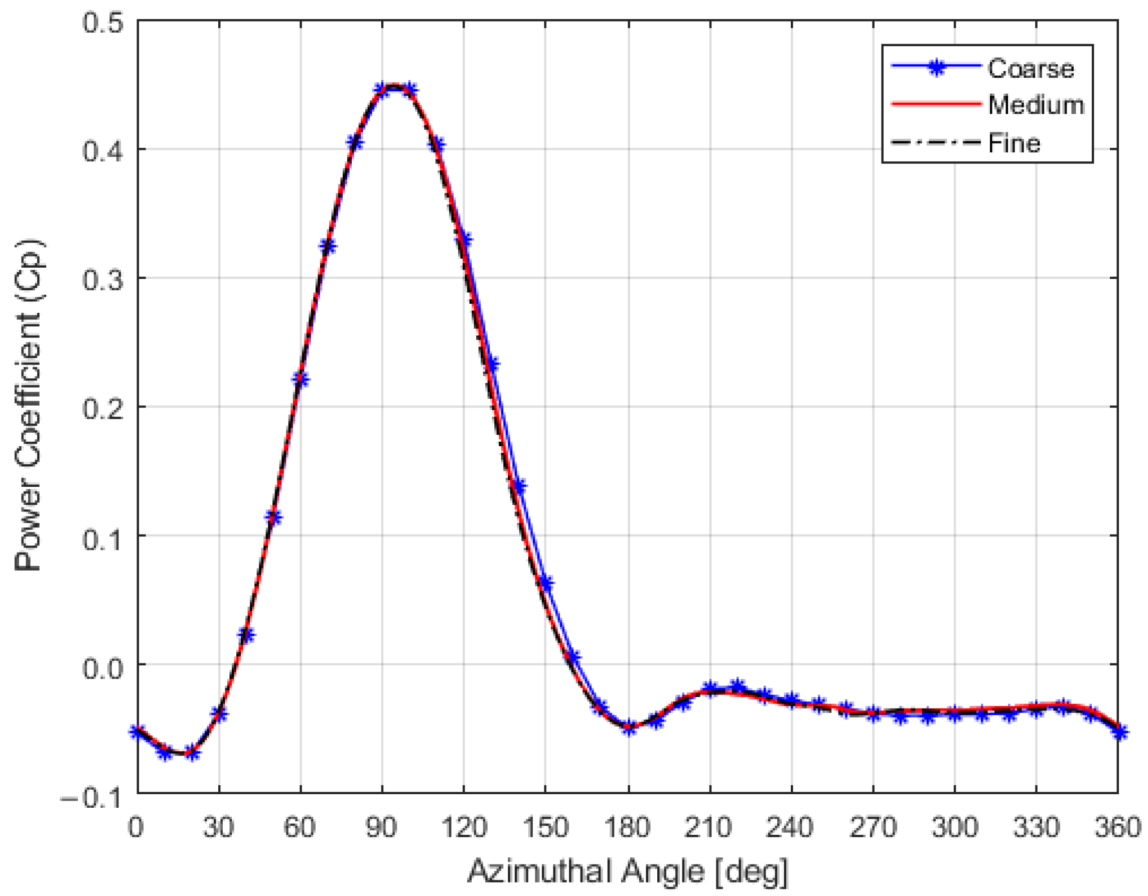
2.4. Sensitivity Test for Grid Size Selection

The ANSYS 2021 R1 meshing tool was used to generate the necessary computational meshes.

Figure 2 reports a detailed vertical cross section of the mesh, showing how the mesh was projected on both the VAWT airfoil and on the near VAWT airfoil space. Likewise, Figure 3 shows the mesh configuration within the control volume. These visual representations provide insight into the discretization of the domain, highlighting the arrangement of mesh cells that play an essential role in helping to calculate and describe the complexities of fluid dynamics during turbine operation.

Furthermore, to proceed with calculations in this study, the frequently technical literature recommended that a Y+ parameter with values ranging from 1 to 5 should be adopted, with this ensuring a detailed near-surface flow resolution, as recommended in [31]. Regarding the mesh quality for 3D simulations, one should mention that orthogonality and skewness metrics revealed less-favorable values at the last cell of the trailing edge. The highest skewness value observed was 0.91, which was slightly smaller than the 0.95 maximum advised. Similarly, the lowest orthogonality value was 0.05, slightly below the recommended minimum of 0.1 [28].

To determine the most suitable mesh size in terms of computational cost and accuracy, three different meshes were tested (see

Table 4. Comparison of the Number of Mesh Elements.

Grid	Total Number of Elements	Cp	% Relative Error
Coarse	873,342	0.172	-
Medium	1,461,327	0.189	9.8%
Fine	2,336,215	0.181	4.2%

Note: Errors are defined as $\% \mathrm{r}\mathrm{e}\mathrm{l}\mathrm{a}\mathrm{t}\mathrm{i}\mathrm{v}\mathrm{e} \mathrm{e}\mathrm{r}\mathrm{r}\mathrm{o}\mathrm{r}={\displaystyle \frac{\mathrm{C}{\mathrm{p}}_{\mathrm{i}}-\mathrm{C}{\mathrm{p}}_{\mathrm{i}+1}}{\mathrm{C}{\mathrm{p}}_{\mathrm{i}}}}$. Subscript i denotes the coarsest mesh, and i + 1 the finest mesh, being evaluated.

) at a constant U∞ = 8 m/s, and at a tip-speed ratio (λ) of 1.4, during six consecutive rotations of the H-Darrieus wind turbine rotor. The sixth rotation was considered as the one providing Cp values, at steady conditions.

The Cp power coefficient, which is a significant indicator of the wind-power utilization and efficiency, was used in this study, to assess the mesh and time-step independence, and can be calculated as follows:

$$\mathit{Cp}={\displaystyle \frac{\mathit{Turbine}\mathit{power}}{\mathit{Wind}\mathit{power}}}={\displaystyle \frac{T·\omega }{\frac{1}{2}\rho U_{\infty }^3\left(DH\right)}}$$

(6)

Figure 4 describes the Cp values obtained when using coarse, medium, and fine meshes, as described in Table 4, for TSR = 1.4, and a march step of 2 degrees.

It is observed that three of the considered meshes yielded stabilized values of Cp, all of them close to each other. However, it was decided to use the finer mesh in all ensuing calculations to ensure the highest possible accuracy.

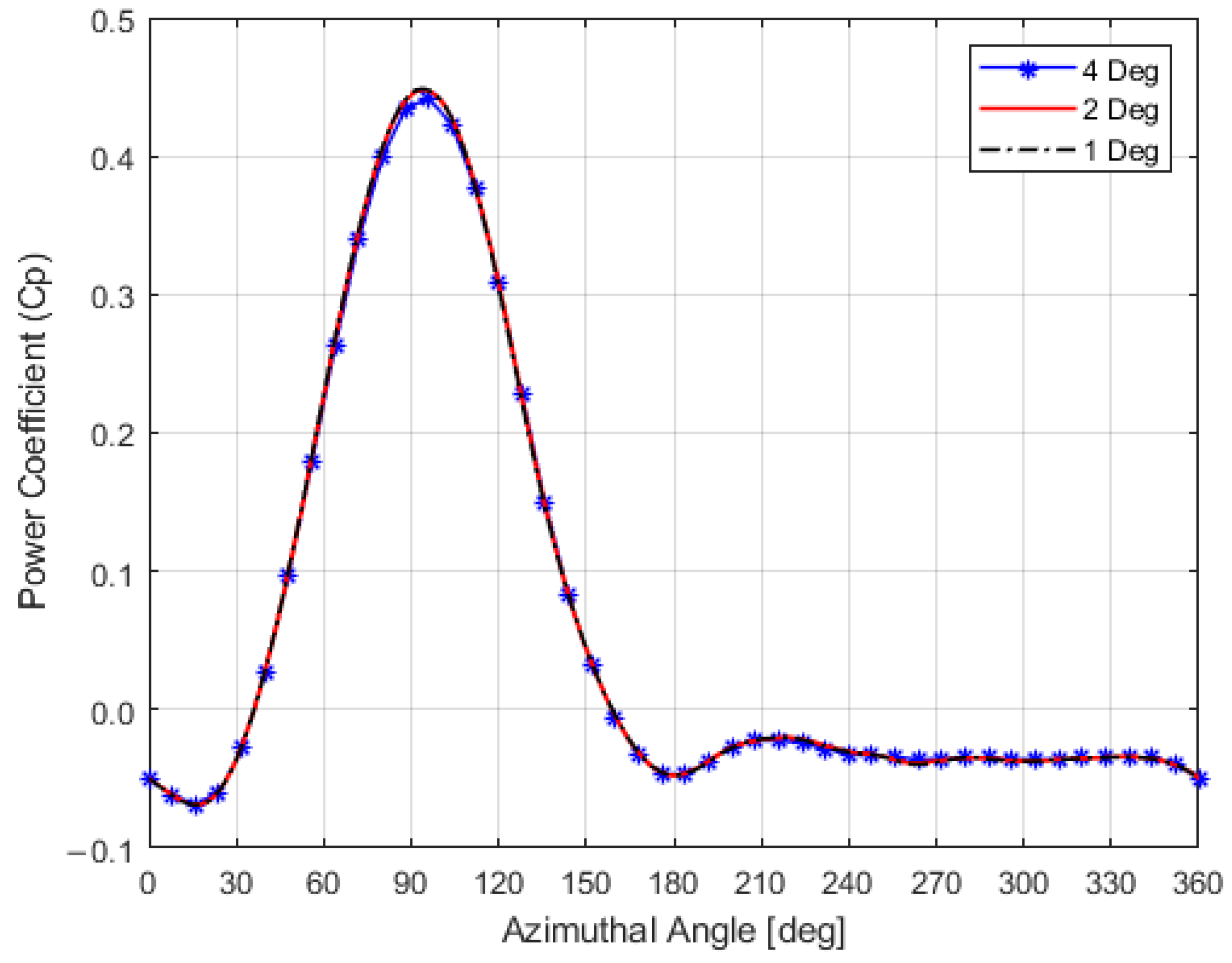
2.5. Sensitivity Test of Time-Step Selection

The selection of the time-step size in unsteady simulations is crucial, as it significantly impacts the results obtained [28]. In the present study, the VAWT simulation was carried out at ${\mathrm{U}}_{\infty }$ = 8 m/s, at a λ = 1.4. This served as the baseline case, as described in Figure 4 and Figure 5. Three different time-step sizes were evaluated, during six consecutive rotations of the H-Darrieus wind turbine rotor. The proposed method was considered reliable for identifying the most appropriate time-step that generated consistent Cp results, while minimizing computational time [28]. This agreed with the findings reported by Ma Ning et al. [21].

Figure 5 reports the results obtained for 0.0025 s, 0.0013 s and 0.0006 s (corresponding to 4°, 2° and 1° angular steps (∆α), respectively). In addition, Figure 5 shows that an angular step of 2° is adequate, given these values are essentially identical to the ones for the 1° angular step. As a result, and in order to reduce the computational time while maintaining satisfactory accuracy, a fine-size mesh, together with a 2° angular time-step, was used for further calculations, in the present study.

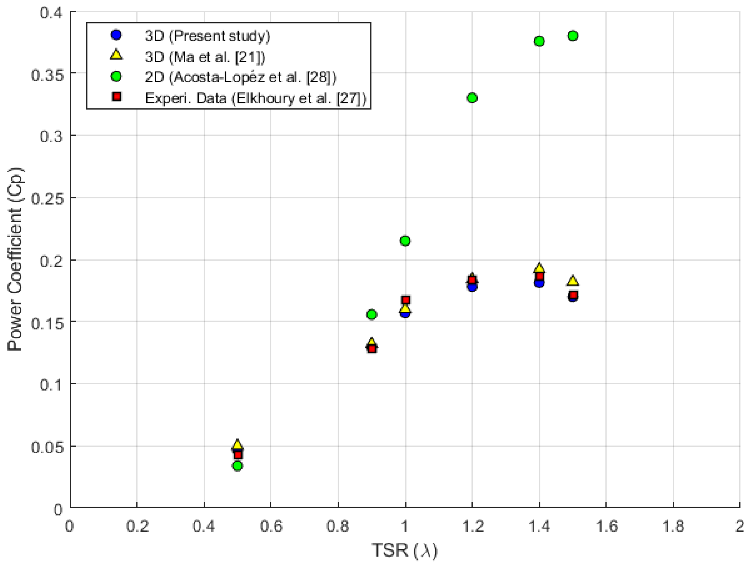
2.6. Comparison with Experimental Data

Figure 6 compares the Cp values at various TSRs, using 2D simulations as reported by Acosta-Lopéz et al. [28], experimental data as shown by Elkhoury et al. [27], and 3D simulations as obtained both by Ma Ning et al. [21] and in the present study. One can observe that the Cps obtained using the 3D models based on the same URANS- SST k-ω model with different mesh configurations are very similar to those of the experimental data from Elkhoury et al. [27]. Moreover, one can also notice that the 3D results of the present study are very close to those obtained with the 2D model of Acosta-Lopéz et al. [28], at TSRs smaller than 0.9 [28], with these values differing considerably at TSRs larger than 0.9 [21,28]. Thus, one can conclude that the consistency of 3D model predictions, with experimental data in the full range of the TSRs, is an excellent indicator of the 3D proposed-model suitability for CFD VAWT analysis.

3. Results and Discussion

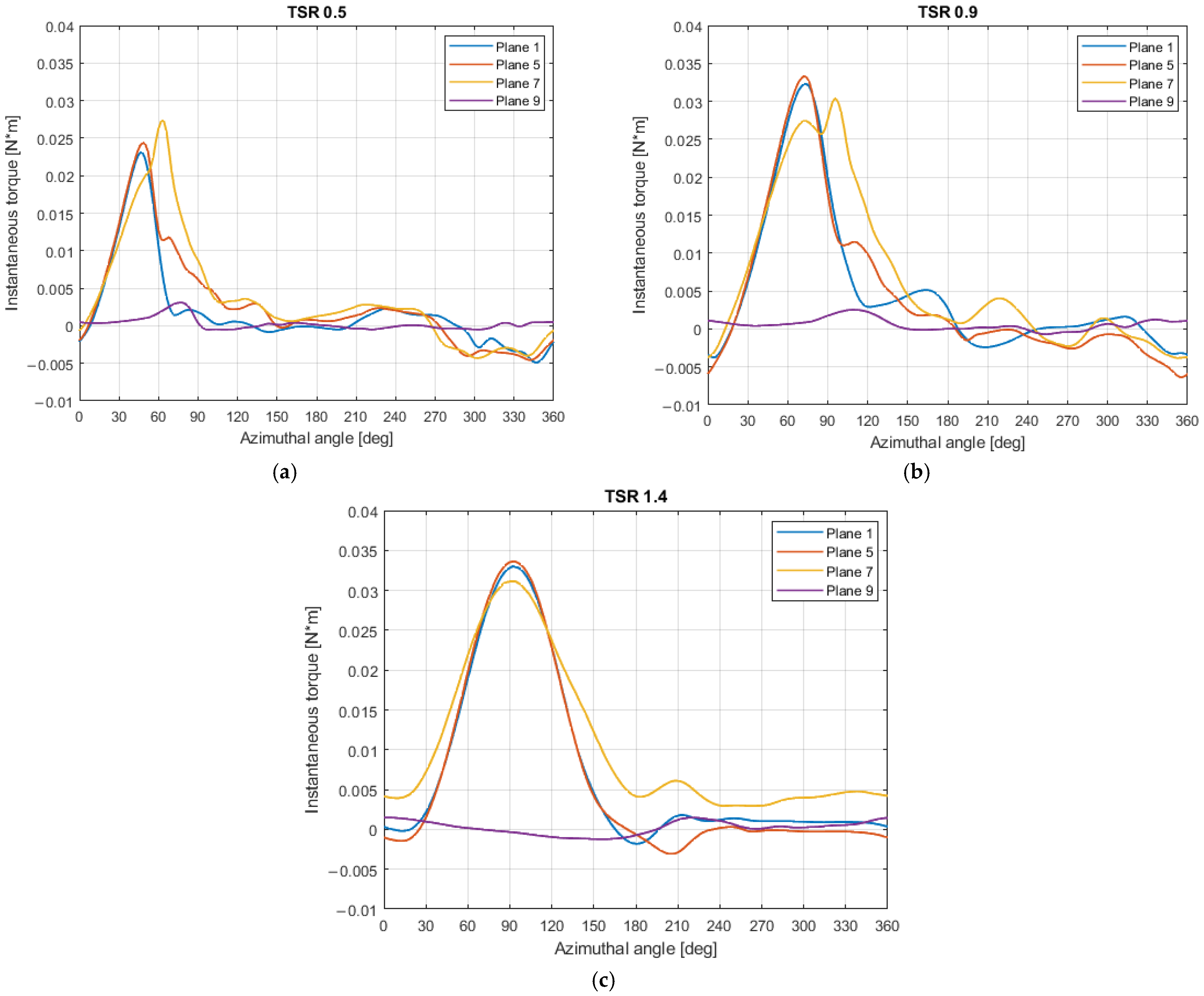
3.1. Influence of Tip Airfoil Losses

To evaluate the influence of tip losses, half of the blade length was divided into nine horizontal planes along its span, with each horizontal plane being separated by 0.05 m. This approach was chosen based on the assumption of airfoil axial-flow symmetry, recognizing that the upper-half blade section displays an identical behavior to the lower-half section. However, and to avoid excessive data reporting, while providing concise results, data reported in the present study were limited to Plane 1 (Z = 0.0 m), Plane 5 (Z = 0.2 m), Plane 7 (Z = 0.3 m), and Plane 9 (Z = 0.4 m), as shown in Figure 7. One should also note that Blade 1 was used as the reference blade for the upcoming analysis.

Furthermore, as proposed by Yichen Jiang et al. [13], the instantaneous torque can be used to analyze the effect of tip losses on the turbine performance. This was carried out, as shown in Figure 8a–c, for three different TSRs (0.5, 0.9, 1.4), which are typical TSR values observed in VAWTs.

Figure 8a reports the instantaneous torque at a TSR of 0.5, from Planes 1 to 9. It can be noticed that for planes 5 and 7 there is a positive effect of the tip vortex, which increases the instantaneous torque, as shown in Figure 8a. This finding could be attributed to a reattachment of the separated flow, induced by the tip vortices, thereby sustaining a leading-edge vortex, at conditions dominated by deep dynamic-stall effects [32]. However, the instantaneous torque at Plane 9, which corresponds to the airfoil edge, exhibits a total torque degradation (Figure 8a–c). Furthermore, when the instantaneous torque was calculated at TSRs of 0.9 and 1.4, a distinct trend emerged across the various horizontal planes. There is, in this respect, a consistent reduction in the extracted torque, as one approaches closer to the blade edge. This trend shows that blade-tip losses tend to diminish the extracted energy, leading to a significantly disturbed flow caused by the vortices at the airfoil tips [13].

One can also conclude that the evaluation of the influence of the tip vortices on the instantaneous torque helps to clarify the differences between 2D- and 3D-model predictions. In 2D simulations, the energy loss caused by the vortex near the blade tip is not accounted for, leading to an overprediction of Cp values. This is a factor that can be addressed through 3D simulations, where more accurate results can be obtained, as previously discussed in Section 2.6 of this article.

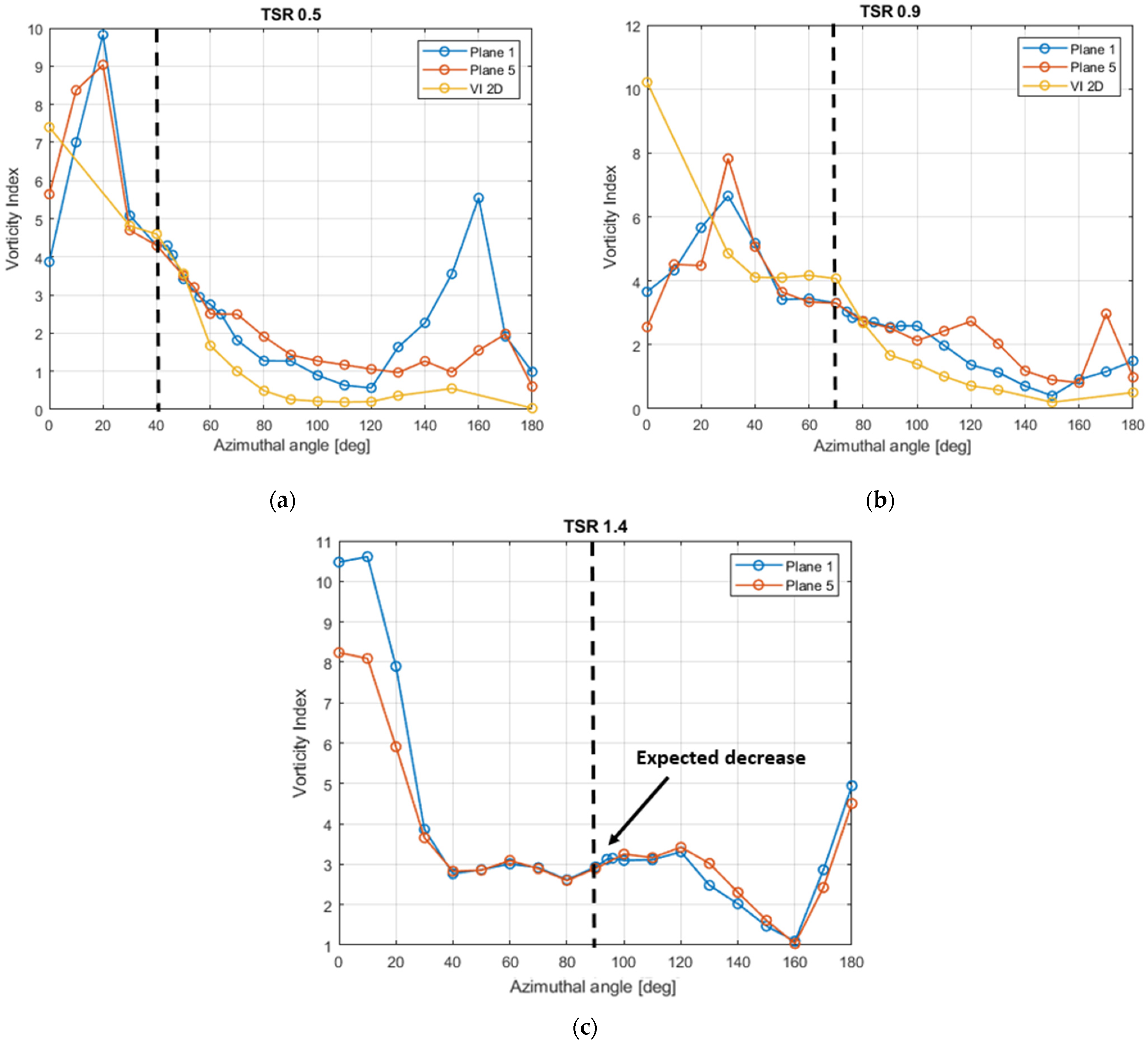
3.2. Vorticity Index in 3D Airfoils

Acosta-Lopéz et al. [28] recently introduced a Vorticity Index to quantitively establish the conditions of maximum torque and vortex separation using the ratio between the maximum vorticity values, at the leading and at the trailing edges (maximum leading-edge vorticity/maximum trailing-edge vorticity). This approach was supported by image analysis at the near air-airfoil H-Darrieus VAWT interface surfaces, and was conducted in the context of a 2D framework.

However, to rigorously assess the Vorticity Index in the context of entire airfoil blade planes, 3D vorticities using the methodology described in Section 3.1, for the various planes of the airfoil (Figure 7) and at different TSRs have to be employed. Figure 9 reports, in respect to this, the maximum vorticities at leading and trailing edges. It can be observed that the highest vorticities (vorticity peaks) occur in the immediate adjacent vicinity of the blade surface, rather than in the bulk of the fluid (Figure 9). It is noteworthy to mention that vorticity values for converged results (six rotations) were always validated, using as the basis sound Cp predictions.

Figure 10a–c, report the Vorticity Index, at two cross-sectional horizontal positions: (a) at Plane 1, located at the central plane, and (b) at Plane 5, which is shifted away from the center plane (Figure 7). These profiles were chosen as a reference, due to the small influence of the disruptive blade-tip effects on them. Moreover, Figure 10 is restricted to 0 to 180 azimuthal angles, given that it is in this domain of angular positions where vortices are detached, and where one observes the largest instantaneous torque values.

As can be seen, in Figure 10a, when comparing the 3D model VIs obtained for Planes 1 and 5, at a TSR = 0.5, to the 2D results, there is a significant vorticity similarity at those planes. The VIs remain constant over an azimuthal range of 30 to 40 degrees, and subsequently decrease. This VI reduction is consistent with the maximum torque observed at the same azimuthal angle range (Figure 8a). Furthermore, a VI reduction is also observed when the TSR increases up to 0.9 (Figure 10b), at a ~70° azimuthal angle (Figure 10b). This VI decay corresponds to the maximum torque observed in Figure 8b. Furthermore, at a TSR of 1.4, VI values stabilize within a wider range (i.e., between azimuthal angles of 40° to 120°), without a sudden decrease in the VI, while agreeing with the maximum torque (Figure 8c). Additionally, one should note that significant phenomenological occurrences like the imminent vortex separation condition, reported by Acosta-Lopéz et al. [28], are not clearly visualized in the 3D framework.

These findings collectively suggest that the efficacy of the 2D simulation appears adequate, as a first approximation, at Plane 1 for TSR values below 1. However, when TSR values exceed the value of 1, there are limitations in the applicability of Vorticity Index analysis, as described above. There are also inconsistencies in the following cases: (a) at a TSR = 0.5, for azimuthal angles larger than 120 degrees, and (b) at a TSR = 1.4, for azimuthal angles larger than 160 degrees. These inconsistencies of VI values that are too large, at these azimuthal angles, expose the limitations of a VI parameter, defined with very low and uncertain vorticity levels at the trailing edge. Thus, as an alternative, in the upcoming manuscript sections a vorticity analysis based on absolute vorticity values is considered more appropriate, instead.

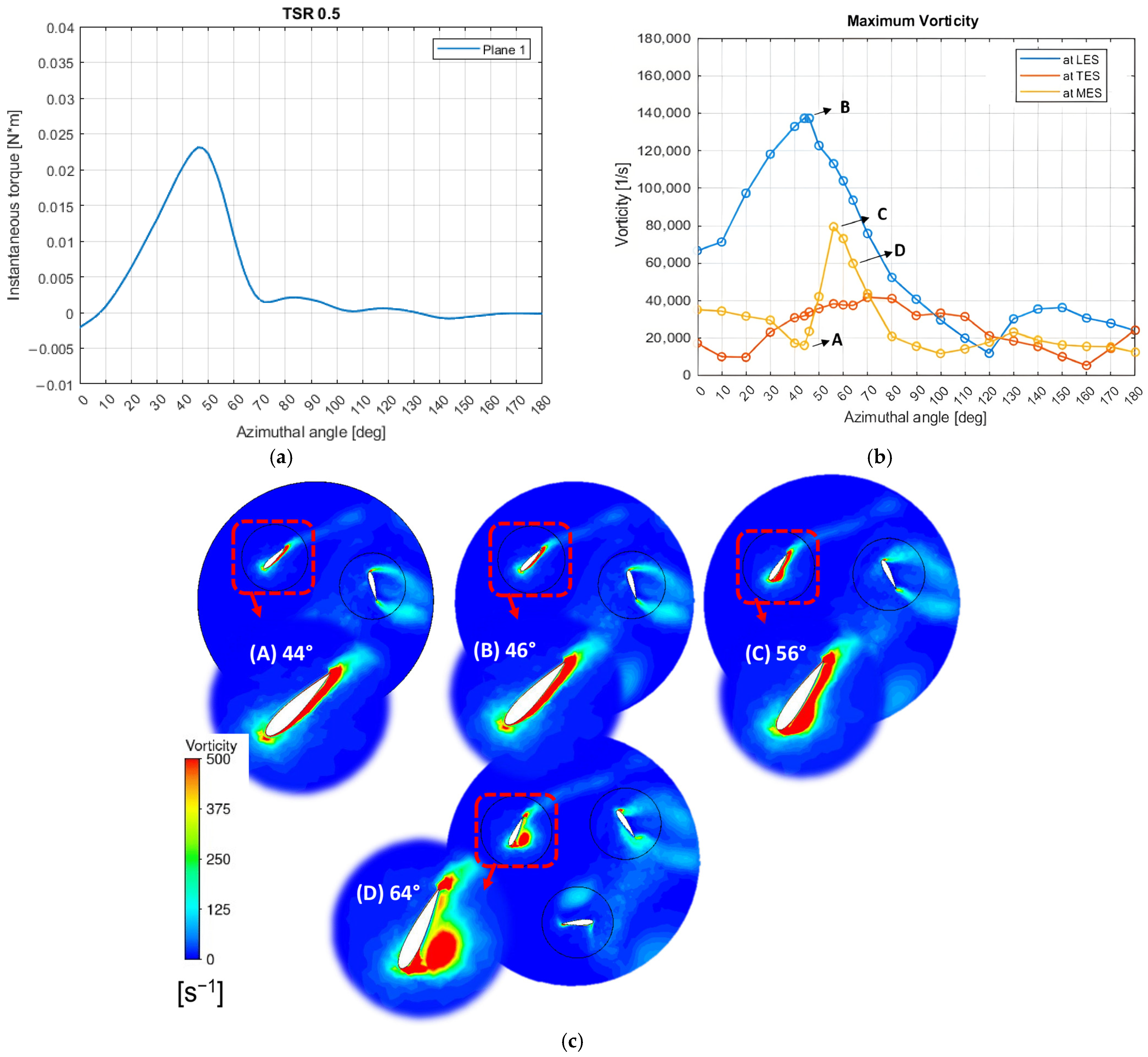
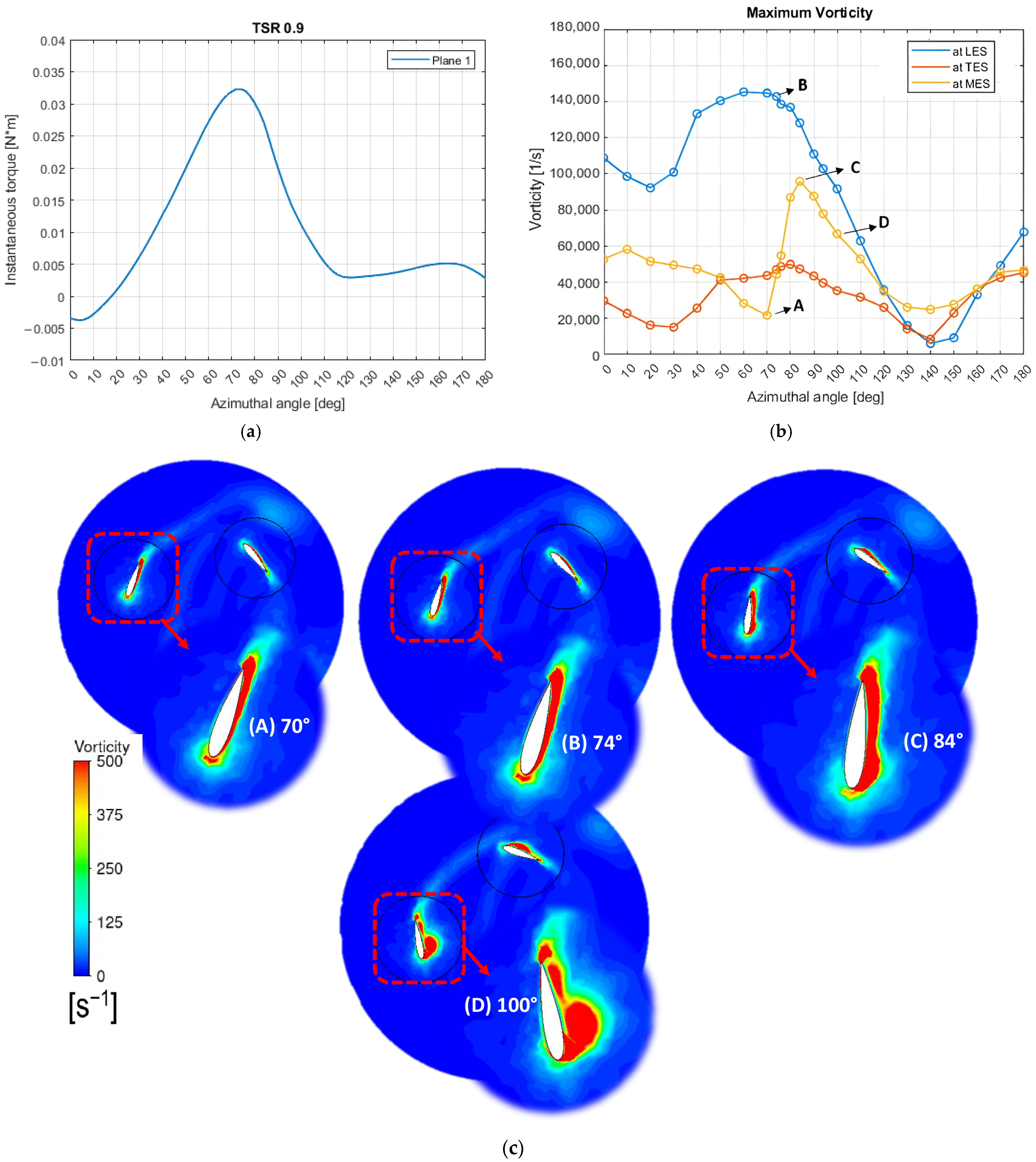
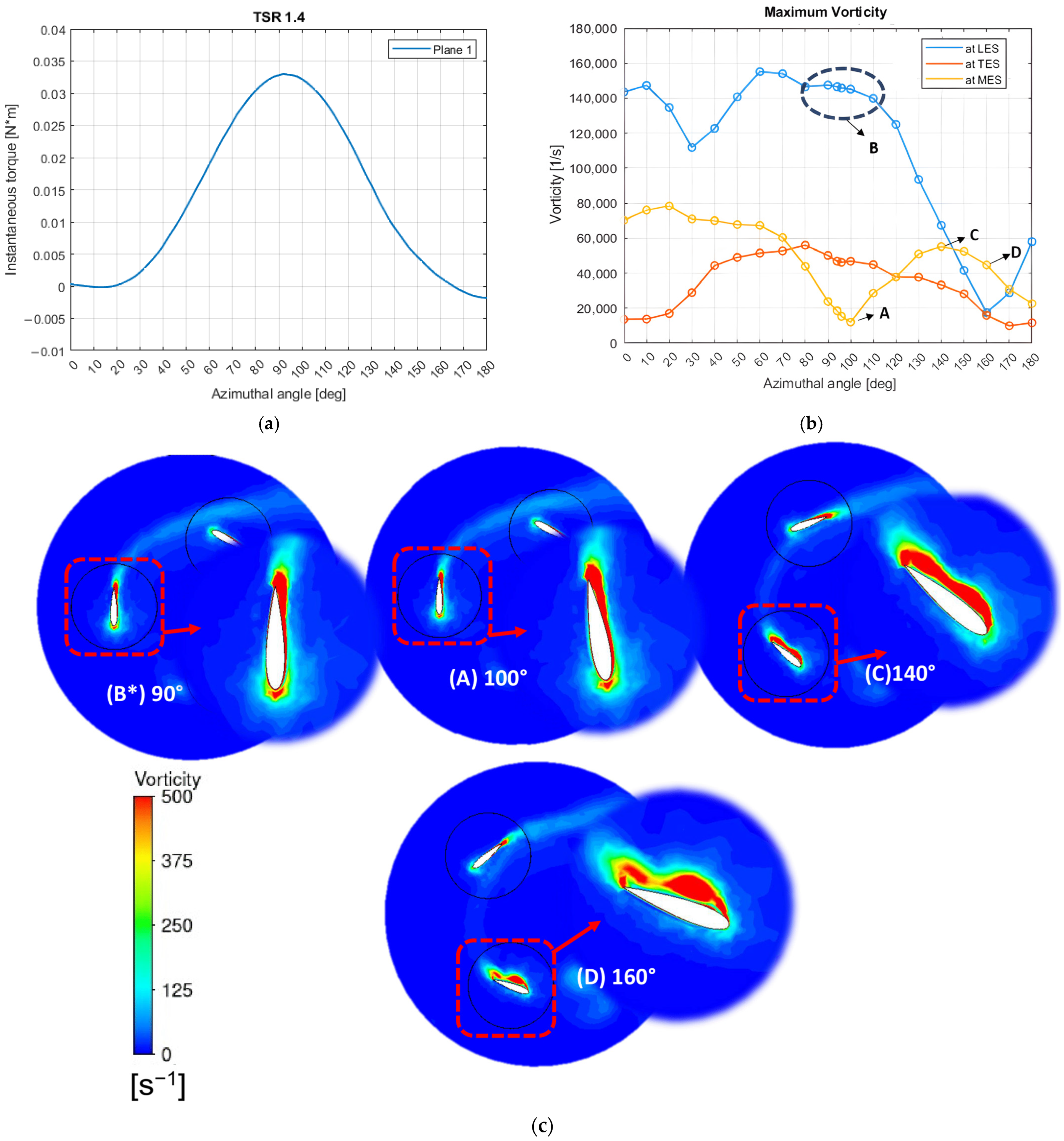
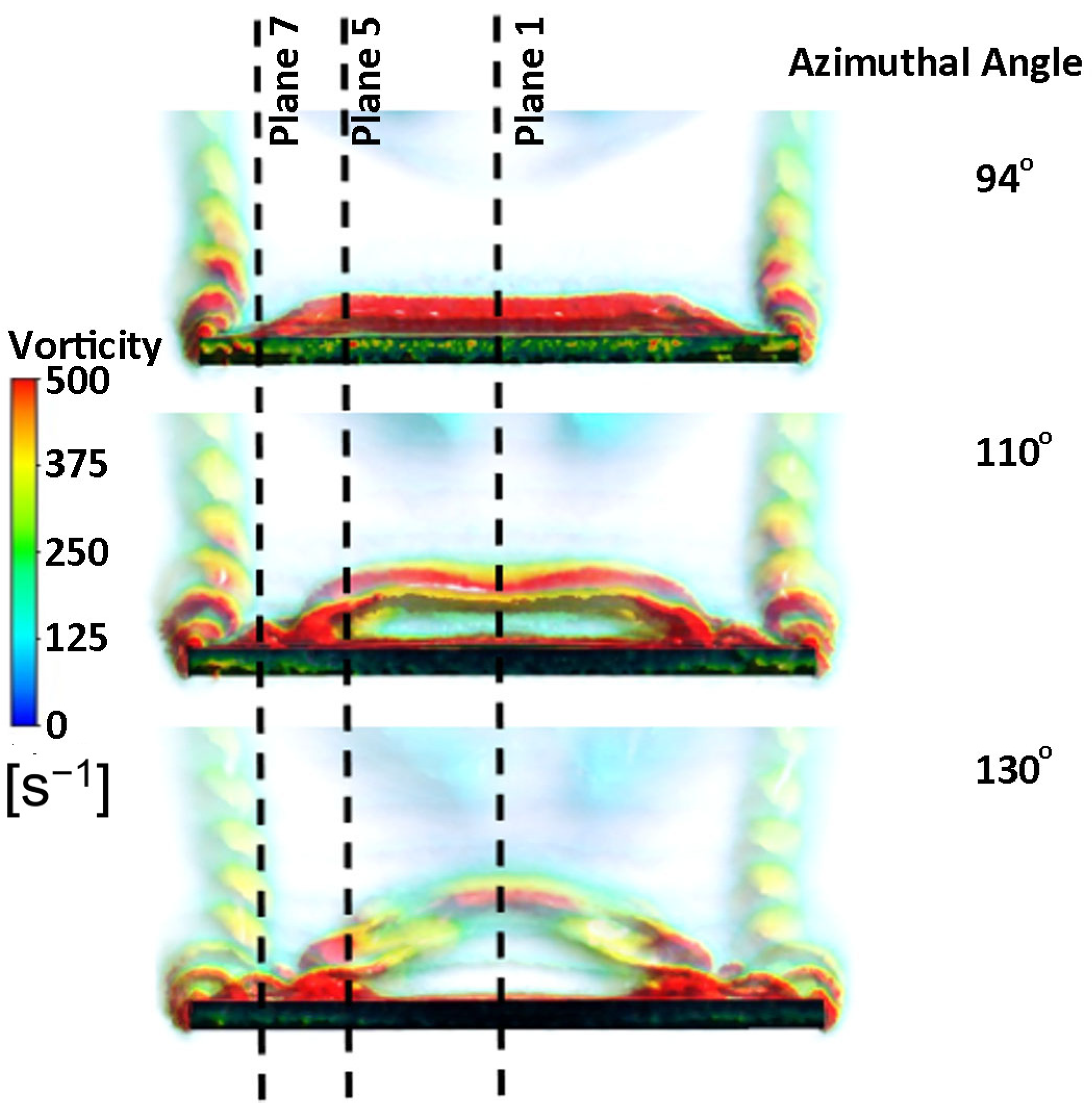
3.3. Vorticity Evaluations in 3D Airfoils

Given the issues with the VI already described, one can conclude that a careful quantitative 3D vorticity analysis is needed. This analysis can be accomplished as described in Figure 11, by employing the following methodology:

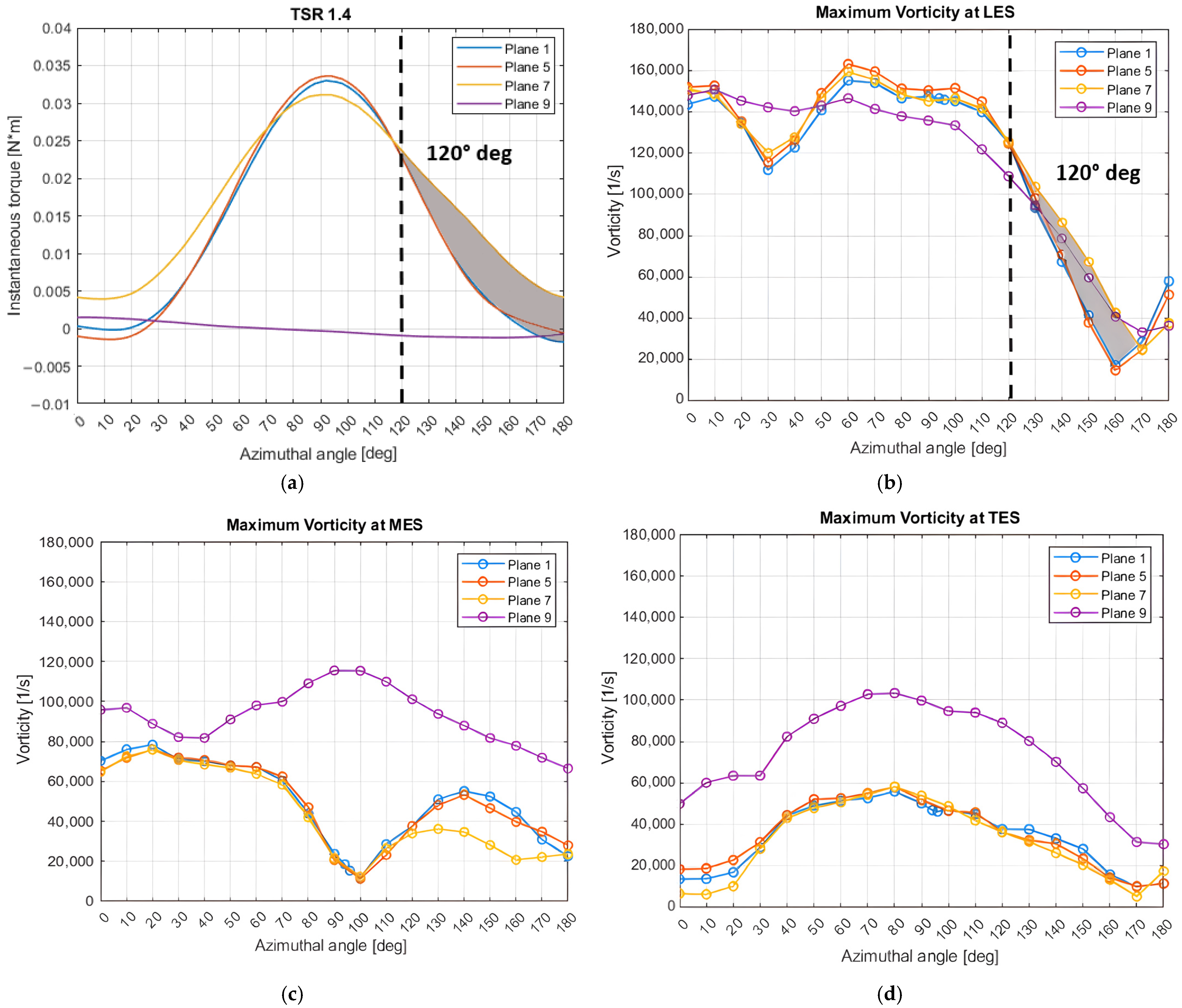
• By evaluating vorticities at the Leading-Edge Section (LES), at the Mid-inner Edge Section (MES), and at the Trailing-Edge Section (TES), to determine the maximum vorticity locus.
• By relating torque and vortex behavior, as proposed by Khaled Souaissa et al. [12], and by assessing this at various cross-sectional planes, along the VAWT axis, as shown in Figure 7.

One should note, in this respect, that vorticity and maximum-vorticity values were analyzed at various planes, at the LES, MES and TES airfoil positions described in Figure 11.

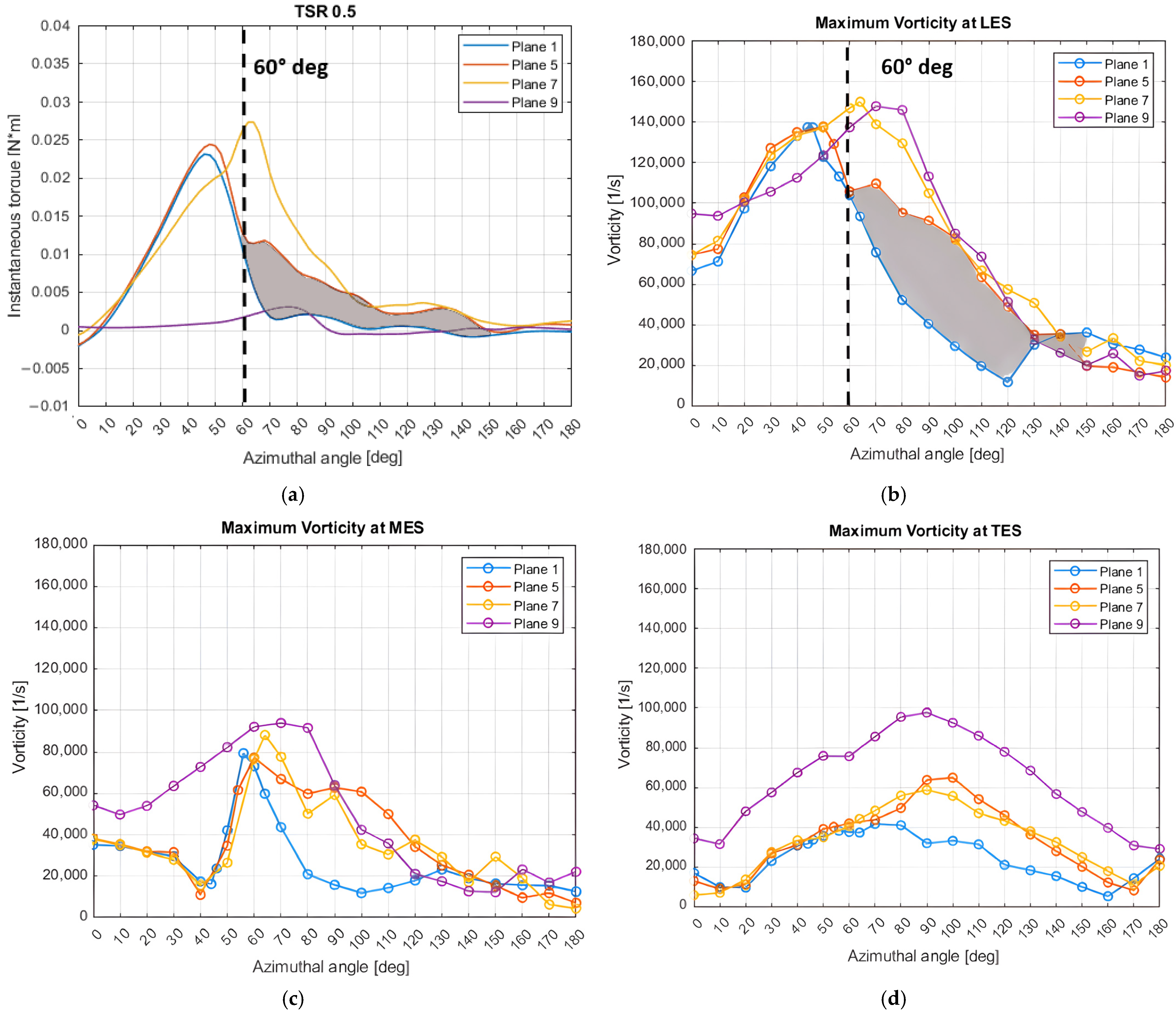
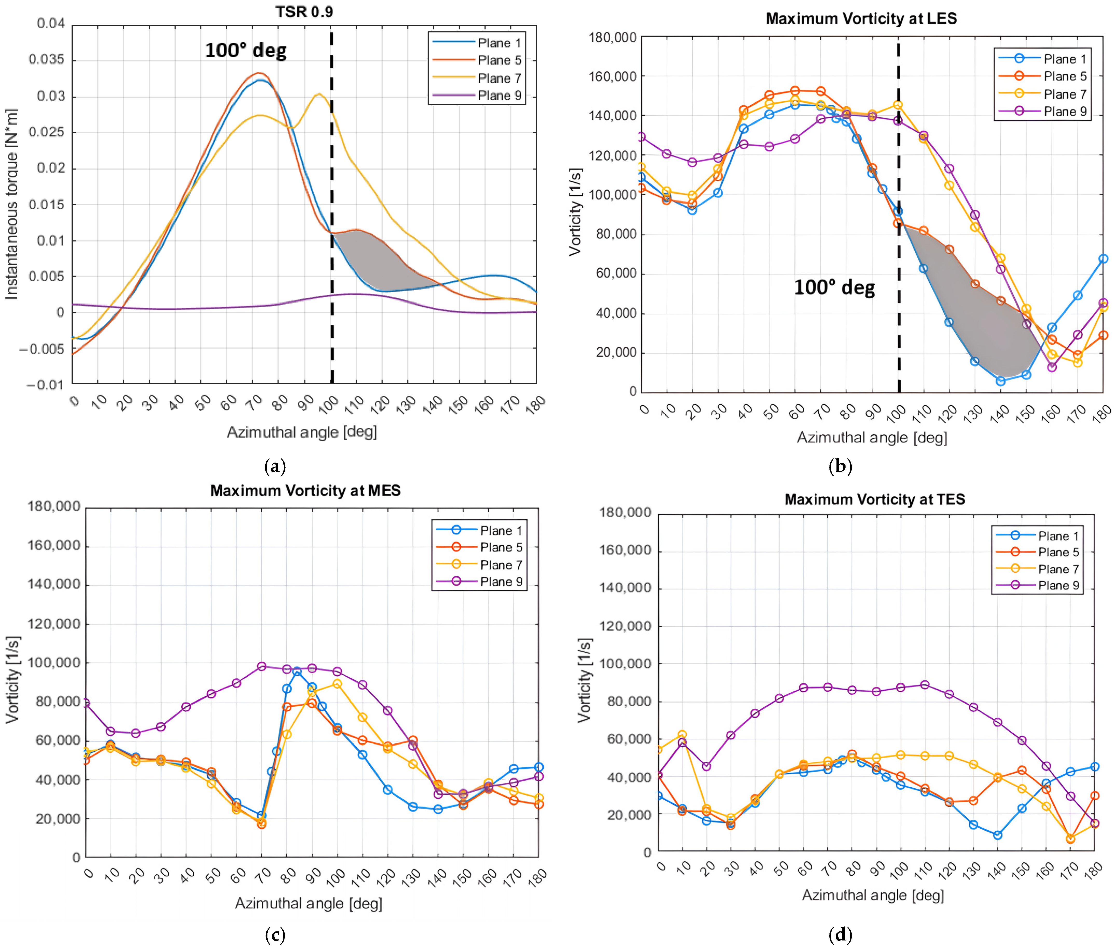
3.3.1. Quantitative 3D Evaluations

Figure 12a, Figure 13a and Figure 14a report the instantaneous torque, while Figure 12b, Figure 13b and Figure 14b depict the near blade-surface maximum vorticities for Plane 1. Additionally, Figure 12c, Figure 13c and Figure 14c illustrate vorticity contours. This analysis is conducted at three different TSR values (0.5, 0.9, and 1.4). Plane 1 was chosen as a reference, due to experiencing minimal blade-tip influence. Moreover, it is anticipated that by utilizing Plane 1, we can delve into the vorticity dynamics near the blade surface, enabling the quantitative determination of the “Imminent Vortex Separation condition” or “the vortex detachment”. This concept is directly related to “Dynamic Stall”, given that, in a VAWT, the rapid changes in the angle of attack result in flow separation and, as this process continues, a leading-edge vortex or “Stall Vortex” travels along the blade surface, from the LE section to the ME section.

Figure 12b, Figure 13b and Figure 14b illustrate maxima vorticity-value profiles (as indicated in Figure 9) over the different blade positions defined in Figure 11. For all TSR conditions, a larger vorticity accumulation is noted at LES, while lower levels of vorticity were noted at MES and TES. This can be attributed to the blade inner-surface coverage during turbine rotation, reducing fluid–surface interactions. Figure 12b, Figure 13b and Figure 14b are a quantitative representation of vorticity accumulation in different blade regions that, later on, can either diffuse or be transported by convection over the blade surface. On the other hand, vorticity contours of Figure 12c, Figure 13c and Figure 14c in the range of 0–500 [s⁻¹] are, therefore, macroscopic observations and the visualization of final fluid-particle rotation resulting from the previously mentioned fluid–surface interactions, which results either in an imminent vortex separation condition and/or fluid vortex detachment. Regarding vorticity as reported in Figure 12b, Figure 13b and Figure 14b, one can notice that the vorticity increases at LES and decreases at MES until points A and B are reached. Beyond conditions A/B, velocity streamlines detach from the blade as the critical angle of attack is surpassed (refer to Appendix A), halting vorticity generation due to the absence of significant fluid viscous interaction, thus causing dynamic stall and LES vorticity reduction. Consequently, vorticity at MES indicates that there is a shift in maximum vorticity values, possibly attributed to either diffusional- or convectional-vorticity transport from LES to MES until point C is attained, where vortex formation and growth starts. Afterwards, vortex detachment should be expected, as becomes visually apparent when using the reported vorticity contours (Figure 12c, Figure 13c and Figure 14c).

It has to be mentioned that these findings align with vorticity dynamics described in [22], where the vorticity boundary layer’s influence on flow is minor, while attachment to the wall remains (as reported in Figure 12, Figure 13, and Figure 14c, prior to conditions A/B). However, and following conditions A/B, intense vorticity significantly affects the flow, leading to local accumulation of vorticity until a maximum value, identified as the C condition or imminent vortex-separation condition, is reached. After the C imminent vortex-separation condition, the vorticity decreases progressively, reaching angular D-range conditions. At these D angular positions, one can observe consistently a fluid vortex detachment.

A similar analysis can be performed by plotting vorticity contours for a TSR of 0.9. In this case, once again, there are four conditions, identified as Conditions A, B, C and D (which are only for visual validation), with the azimuthal angles being reported in Figure 13a–c, as follows: (a) Condition A is seen in the MES, at a 70° azimuthal angle, (b) Condition B occurs in the LES, at a 74° azimuthal angle, (c) Condition C takes place at MES, at an 84° azimuthal angle, and (d) Condition D is seen in the LES, at azimuthal angles larger than 84°. Thus, one can observe that when the TSR is increased from 0.5 to 0.9, Conditions A, B, C and D are still present. However, for a TSR = 0.9, these conditions are shifted to significantly larger azimuthal angles, with the vortex detachment being a phenomenon that is still clearly observable.

Finally, for a TSR of 1.4 (Figure 14a–c), there are significant differences in flow patterns, as observed for TSRs of 0.5 and 0.9. Conditions A, B, C, and D are still observable at a TSR = 1.4. However, these characteristic conditions fall in a range of azimuthal angles, with the air still remaining attached to the airfoil, and this due to the larger angles of attack.

One can observe in Figure 14c that (i) Condition “A” occurs in the MES, at a 100° azimuthal angle, (ii) Condition “B” appears in the LES, in a range between 80 and 110° azimuthal angles, (iii) Condition “C” takes place in the MES, at a 140° azimuthal angle, and (iv) Condition “D” is seen in the LES, at azimuthal angles larger than 140°. However, it is noteworthy to mention that in this last case there is a significantly delayed vortex separation. These characteristic phenomena involving a lack of vortex separation, at TSRs > 1.4, can be linked to dynamic stall, as discussed in previous references [11].

To provide adequate information on the performance of the vertical turbine, it is necessary to complement the previous vorticity analysis (Plane 1) with results at Planes 5, 7 and 9, where fluid flow is significantly airfoil-edge disturbed, and vortex detachment via 3D data analysis is not readily apparent. As depicted in Figure 15, this phenomenon, resulting in the formation of arc-like structures [14], shows the difference in vorticities generated at planes 5, 7 and 9 (for a given fluid flow). In these cases, the vorticities are significantly disturbed by the airfoil tips.

3.3.2. Vorticity and Torque Relationship

Exploring the connection between vorticity and torque holds significant importance in the context of turbine performance. In the preceding section, it is clarified how vorticity generation and propagation contribute to the emergence of vortex structures, as depicted in Figure 12c, Figure 13c and Figure 14c. Understanding this process is crucial, given it not only provides insights into the aerodynamics of the system but also serves as a key indicator of dynamic-stall conditions. According to this analysis, dynamic stall, marked by the fluid’s inability to remain attached to the blade surface, can be inferred from vorticity patterns. An understanding of these matters can guide the approaches for enhancing improvements in turbine efficiency.

Figure 16a,b, Figure 17a,b and Figure 18a,b report the vorticity patterns across different planes as discussed in Section 3.1, and for TSRs of 0.5, 0.9 and 1.4.

For example, when comparing Figure 16b and Figure 17b, trends in vorticity and torque values between Plane 1 and Plane 5 display notable similarity. Up to 60 degrees for a TSR of 0.5, and up to 100 degrees for a TSR of 0.9, the values remain nearly identical. Beyond these angles, however, the vorticity values at Plane 5 begin to supersede those from Plane 1, which is attributed to the delayed formation of the tip vortex compared to the mid-blade vortex [13,17]. Despite variations in the torque–vorticity relationship for each respective plane (due to the delayed vortex formation), a clear connection between these two parameters persists. Additionally, when examining the vorticity values obtained at Plane 7, at a TSR of 0.5, one can notice that these values are similar to those of Plane 1 and 5, while being obtained, however, over a more greatly extended azimuthal-angle range, with this being assigned to a delayed dynamic-stall angle of attack occurring in those planes. This extended range or lag in flow-separation conditions results in higher torque values.

Figure 18a,b report the instantaneous torque at Planes 1 and Plane 7, for a TSR = 1.4. Plots with shaded areas for Planes 1 and 7 allow adequate visualization of torque and vorticity differences. It should be noted that the instantaneous torque differences between Planes 1 and 5 are too small to be clearly reported, as shown in Figure 18b.

As shown in Figure 18a,b, for a TSR of 1.4, the vorticity values at Plane 7 are consistent throughout a more extended azimuthal-angle range, during the entire vertical airfoil rotation. These prolonged, stable and elevated vorticity values explain the generation of higher torques. When analyzing vorticity values and instantaneous torques at a TSR of 1.4, including those occurring at Plane 9 (the vertical edge of the airfoil), one can also observe that, despite the good vorticity stability along the airfoil, there is a drop in the instantaneous torque at the very last airfoil horizontal section (very close to the vertical edge of the airfoil). This is significant in order to corroborate the calculated and reduced Cp values (refer to Figure 6) obtained with the 3D model of the present study.

Although the trends in vorticity at the Middle-Edge Segment (MES) and at the Trailing-Edge Segment (TES) (Figure 16c,d, Figure 17c,d and Figure 18c,d) are not as discernible in relation to the torque behavior, as seen in the case of the Leading-Edge Segment (LES), there is still an observable evidence of vortex migration from the LES to the MES.

It is worth noting that although the vorticity values at Plane 9 for the three TSR conditions assessed in this study are comparable to those of the other planes, the torque extraction is much lower than those of the others (see Figure 16a–d, Figure 17a–d and Figure 18a–d). This can be attributed to the vorticity released to the surrounding airfoil environment, which occurs without providing any harnessed energy to the airfoil body. This is primarily because Plane 9 is located exactly at the very airfoil edge.

From Section 3.3.2. results, two design recommendations arise:

(i)

Reducing the tip vortex effect is crucial to improve the overall power coefficient while minimizing torque drop, as shown in Figure 16a, Figure 17a, and Figure 18a, and a more effective design should consider two key ideas. Firstly, increasing the H/R aspect ratio improves turbine performance by reducing aerodynamic losses, such as wingtip vortices, which affect a smaller portion of the blade [33]. Secondly, refining the wing design or incorporating winglets can effectively mitigate these vortices [13].

(ii)

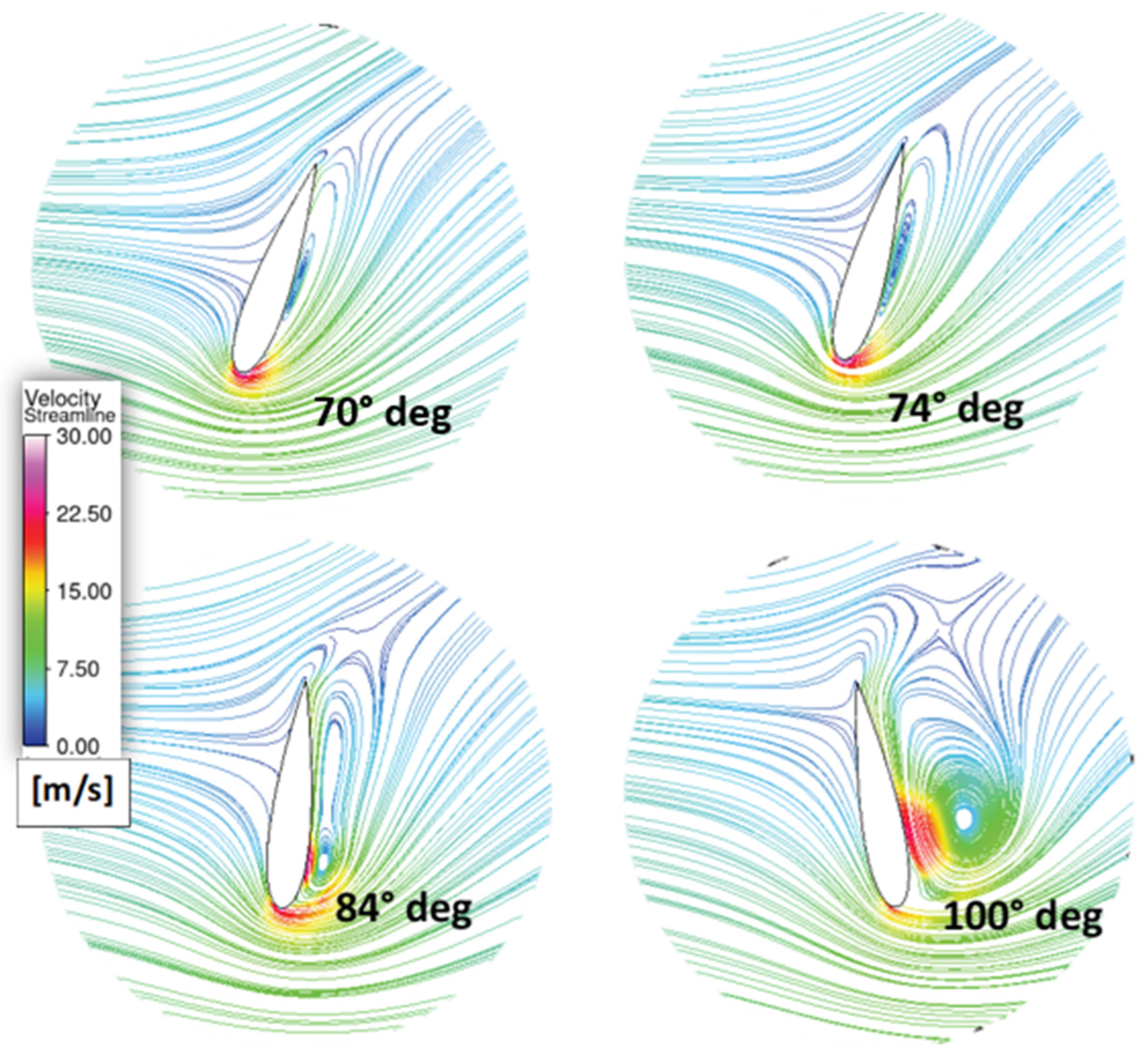
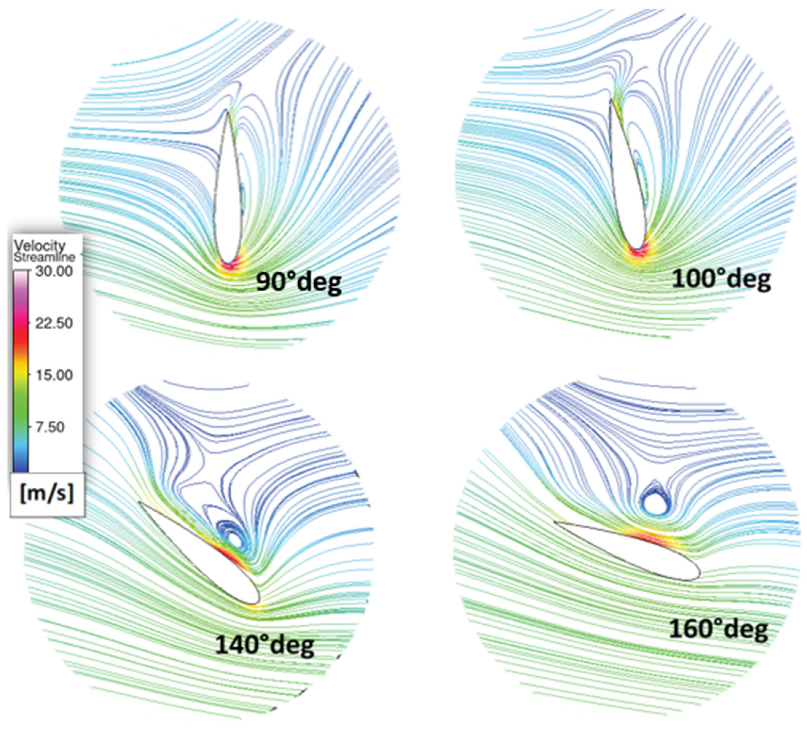
Maintaining high vorticity values at the LES. This notion is in agreement with current approaches, such as the angle-of-attack variation [25,26], aiming to delay the dynamic stall or vortex shedding, or by using micro vortex-generator techniques. These micro vortex generators, among other active/passive control devices, create small vortices that help to energize the flow, preventing a vortex separation [34,35]. All these approaches converge on the same principle: prolonging fluid adherence to the surface, which results in elevated vorticity at the blade’s surface, avoiding massive flow separation.

4. Conclusions

• Torque calculations at various airfoil planes using 3D models, with assessment of the overall torque in VAWTs, can be validated with experimentally measured Cp values at various TSRs in the 0.5–1.4 range.
• VAWT fluid dynamics employing 3D models is essential for calculating instantaneous torque and the amount of energy lost as a result of vortex shedding, at the airfoil tips.
• VAWT fluid dynamics using 3D models needs to be used to develop instantaneous vorticity and instantaneous torque calculations, at various chord positions such as the LES (Leading-Edge Section), the MES (Medium-Edge Section) and the TES (Trailing-Edge Section).
• Determining quantitatively the vorticity patterns during turbine operation provides valuable insights into vortex dynamics, dynamic stall, and the identification of the imminent vortex-separation condition (IVSC). Understanding these patterns is essential for refining analysis techniques and optimizing turbine efficiency.
• VAWT fluid-dynamic analysis using 3D models is valuable in order to postulate a distinctive correlation between torque and vorticity values, with this relationship being a function of the axial and chord positions of the airfoil.

References

1. Environmental and Energy Study Institute. Available online: https://www.eesi.org/topics/fossil-fuels/description (accessed on 25 August 2023).
2. Rapier, R. BP Review: New Highs in Global Energy Consumption and Carbon Emissions in 2019. Forbes, 20 June 2020. Available online: https://www.forbes.com/sites/rrapier/2020/06/20/bp-review-new-highs-in-global-energy-consumption-and-carbon-emissions-in-2019/?sh=692c741466a1 (accessed on 25 August 2023).
3. Gerrie, C.; Islam, S.Z.; Gerrie, S.; Turner, N.; Asim, T. 3D CFD modelling of performance of a vertical axis turbine. Energies 2023, 16, 1144. [Google Scholar] [CrossRef]
4. Boldyrev, A.A.; Herasymenko, N.V. The Usage of Solar Panels Advantages and Disadvantages. Doctoral Dissertation, BHTУ, Vinnytsia, Ukraine, 2020. Available online: http://ir.lib.vntu.edu.ua//handle/123456789/29940 (accessed on 30 September 2023).
5. Vinoth Kanna, I.; Paturu, P. A study of hydrogen as an alternative fuel. Int. J. Ambient Energy 2020, 41, 1433–1436. [Google Scholar] [CrossRef]
6. Benghanem, M.; Mellit, A.; Almohamadi, H.; Haddad, S.; Chettibi, N.; Alanazi, A.M.; Dasalla, D.; Alzahrani, A. Hydrogen production methods based on solar and wind energy: A review. Energies 2023, 16, 757. [Google Scholar] [CrossRef]
7. Mohtasham, J. Renewable Energies. Energy Procedia 2015, 74, 1289–1297. [Google Scholar] [CrossRef]
8. Schubel, P.J.; Crossley, R.J. Wind Turbine Blade Design Review. Wind Eng. 2012, 36, 365–388. [Google Scholar] [CrossRef]
9. Li, S.; Dai, Y. Design and Simulation Analysis of a Small-Scale Compressed Air Energy Storage System Directly Driven by Vertical Axis Wind Turbine for Isolated Areas. J. Energy Eng. 2015, 141, 04014032. [Google Scholar] [CrossRef]
10. Ferreira, C.S.; Bijl, H.; van Bussel, G.; Van Kuik, G. Simulating Dynamic Stall in a 2D VAWT: Modeling Strategy, Verification and Validation with Particle Image Velocimetry Data. J. Phys. Conf. Ser. 2007, 75, 012023. [Google Scholar] [CrossRef]
11. Le Fouest, S.; Mulleners, K. The Dynamic Stall Dilemma for Vertical-Axis Wind Turbines. Renew. Energy 2022, 198, 505–520. [Google Scholar] [CrossRef]
12. Souaissa, K.; Ghiss, M.; Chrigui, M.; Bentaher, H.; Maalej, A. A Comprehensive Analysis of Aerodynamic Flow around H-Darrieus Rotor with Camber-Bladed Profile. Wind Eng. 2019, 43, 459–475. [Google Scholar] [CrossRef]
13. Jiang, Y.; He, C.; Zhao, P.; Sun, T. Investigation of Blade Tip Shape for Improving VAWT Performance. J. Mar. Sci. Eng. 2020, 8, 225. [Google Scholar] [CrossRef]
14. Visbal, M.R.; Garmann, D.J. Dynamic stall of a finite-aspect-ratio wing. AIAA J. 2019, 57, 962–977. [Google Scholar] [CrossRef]
15. Bianchini, A.; Balduzzi, F.; Bachant, P.; Ferrara, G.; Ferrari, L. Effectiveness of two-dimensional CFD simulations for Darrieus VAWTs: A combined numerical and experimental assessment. Energy Convers. Manag. 2017, 136, 318–328. [Google Scholar] [CrossRef]
16. Balduzzi, F.; Drofelnik, J.; Bianchini, A.; Ferrara, G.; Ferrari, L.; Campobasso, M.S. Darrieus wind turbine blade unsteady aerodynamics: A three-dimensional Navier-Stokes CFD assessment. Energy 2017, 128, 550–563. [Google Scholar] [CrossRef]
17. Balduzzi, F.; Bianchini, A.; Maleci, R.; Ferrara, G.; Ferrari, L. Critical issues in the CFD simulation of Darrieus wind turbines. Renew. Energy 2016, 85, 419e35. [Google Scholar] [CrossRef]
18. Fertahi, S.E.-D.; Samaouali, A.; Kadiri, I. CFD Comparison of 2D and 3D Aerodynamics in H-Darrieus Prototype Wake. e-Prime—Adv. Electr. Eng. Electron. Energy 2023, 4, 100178. [Google Scholar] [CrossRef]
19. Nazari, S.; Zamani, M.; Moshizi, S.A. Comparison between two-dimensional and three-dimensional computational fluid dynamics techniques for two straight-bladed vertical-axis wind turbines in inline arrangement. Wind Eng. 2018, 42, 647–664. [Google Scholar] [CrossRef]
20. Franchina, N.; Persico, G.; Savini, M. 2D-3D Computations of a Vertical Axis Wind Turbine Flow Field: Modeling Issues and Physical Interpretations. Renew. Energy 2019, 136, 1170–1189. [Google Scholar] [CrossRef]
21. Ma, N.; Lei, H.; Han, Z.; Zhou, D.; Bao, Y.; Zhang, K.; Zhou, L.; Chen, C. Airfoil Optimization to Improve Power Performance of a High-Solidity Vertical Axis Wind Turbine at a Moderate Tip Speed Ratio. Energy 2018, 150, 236–252. [Google Scholar] [CrossRef]
22. Kheradvar, A.; Pedrizzetti, G. Vortex dynamics. In Vortex Formation in the Cardiovascular System; Springer: London, UK, 2012; pp. 17–44. [Google Scholar]
23. Wu, J.Z.; Ma, H.Y.; Zhou, M.D. Vorticity and Vortex Dynamics; Springer Science & Business Media: Berlin/Heidelberg, Germany, 2007. [Google Scholar]
24. Wu, J.C. Elements of Vorticity Aerodynamics; Springer: Berlin/Heidelberg, Germany, 2018. [Google Scholar]
25. Sagharichi, A.; Maghrebi, M.J.; ArabGolarcheh, A. Variable Pitch Blades: An Approach for Improving Per-formance of Darrieus Wind Turbine. J. Renew. Sustain. Energy 2016, 8, 053305. [Google Scholar] [CrossRef]
26. Sagharichi, A.; Zamani, M.; Ghasemi, A. Effect of solidity on the performance of variable-pitch vertical axis wind turbine. Energy 2018, 161, 753–775. [Google Scholar] [CrossRef]
27. Elkhoury, M.; Kiwata, T.; Aoun, E. Experimental and Numerical Investigation of a Three-Dimensional Vertical-Axis Wind Turbine with Variable-Pitch. J. Wind Eng. Ind. Aerodyn. 2015, 139, 111–123. [Google Scholar] [CrossRef]
28. Acosta-López, J.G.; Blasetti, A.P.; Lopez-Zamora, S.; de Lasa, H. CFD Modeling of an H-Type Darrieus VAWT under High Winds: The Vorticity Index and the Imminent Vortex Separation Condition. Processes 2023, 11, 644. [Google Scholar] [CrossRef]
29. Wikipedia Contributors. “Navier–Stokes Equations”. Wikipedia, The Free Encyclopedia. Available online: https://en.wikipedia.org/wiki/Navier–Stokes_equations (accessed on 25 August 2023).
30. Menter, F.R. Two-Equation Eddy-Viscosity Turbulence Models for Engineering Applications. AIAA J. 1994, 32, 1598–1605. [Google Scholar] [CrossRef]
31. Wong, K.H.; Chong, W.T.; Poh, S.C.; Shiah, Y.-C.; Sukiman, N.L.; Wang, C.-T. 3D CFD Simulation and Parametric Study of a Flat Plate Deflector for Vertical Axis Wind Turbine. Renew. Energy 2018, 129 Pt A, 32–55. [Google Scholar] [CrossRef]
32. Dong, L.; Choi, K.S.; Mao, X. Interplay of the Leading-Edge Vortex and the Tip Vortex of a Low-Aspect-Ratio Thin Wing. Exp. Fluids 2020, 61, 200. [Google Scholar] [CrossRef]
33. Naccache, G.; Paraschivoiu, M. Development of the dual vertical axis wind turbine using computational fluid dynamics. J. Fluids Eng. 2017, 13, 121105. [Google Scholar] [CrossRef]
34. Yan, Y.; Avital, E.; Williams, J.; Cui, J. CFD Analysis for the Performance of Micro-Vortex Generator on Aerofoil and Vertical Axis Turbine. J. Renew. Sustain. Energy 2019, 11, 043302. [Google Scholar] [CrossRef]
35. Syawitri, T.P.; Yao, Y.; Yao, J.; Chandra, B. A Review on the Use of Passive Flow Control Devices as Performance Enhancement of Lift-Type Vertical Axis Wind Turbines. Wiley Interdiscip. Rev. Energy Environ. 2022, 11, e435. [Google Scholar] [CrossRef]
Figure 1. (a) Schematic description of a Darrieus-H wind turbine. (b) Computational fixed and rotating domains adopted for CFD calculations.
Processes 12 01556 g001
Figure 2. Projection of the mesh considered in simulations both in the airfoil and in the near-airfoil region.
Processes 12 01556 g002
Figure 3. Representation of the 3D computational mesh of the hexahedral domain used in the present study.
Processes 12 01556 g003
Figure 4. Mesh dependency (Cp values for Blade 1 at a TSR = 1.4, and a 2° march time-step).
Processes 12 01556 g004
Figure 5. Time-step dependency (Cp values for Blade 1, at a TSR = 1.4, and using fine-size mesh).
Processes 12 01556 g005
Figure 6. Comparison of Cp values obtained with 2D and 3D models and experimental data.
Processes 12 01556 g006
Figure 7. Horizontal-section planes, at the various vertical-airfoil levels considered in this study.
Processes 12 01556 g007
Figure 8. Instantaneous torque obtained at different airfoil axial positions: (a) TSR = 0.5, (b) TSR = 0.9 and (c) TSR = 1.4.
Processes 12 01556 g008
Figure 9. Snapshot of vorticity values at Plane 1 (TSR = 0.5). Notes: (a) the angles of 70, 190, and 310 degrees correspond to the positions of blades 1, 2, and 3, respectively, during the time of vorticity evaluations. (b) X and Y refer to the actual position of airfoil elements at Plane 1, using Cartesian coordinates.
Processes 12 01556 g009
Figure 10. Vorticity Index for Blade 1, in 3D, at Plane 1 and Plane 5: (a) TSR = 0.5, (b) TSR = 0.9, (c) TSR = 1.4. Note: 2D results for TSR = 1.4 are not reported, given the lack of confidence with the CP predictions, as reported in Figure 6.
Processes 12 01556 g010
Figure 11. Cross-section of the airfoil showing the LES, the MES, the TES, at Plane 1. Notes: (a) LES corresponds to 10% of the chord length, (b) MES corresponds to 80% of the chord length, and (c) TES corresponds to 10% of the chord length.
Processes 12 01556 g011
Figure 12. (a). Instantaneous torque (Plane 1-TSR = 0.5). (b). Maximum vorticity at the leading edge, the mid inner-edge, and the trailing edge (Plane 1-TSR = 0.5). (c). Vorticity contours at TSR = 0.5 for the following azimuthal angles: (A) 44°, (B) 46°, (C) 56° and (D) 64°. Notes: (i) The wind direction is horizontal from left to right, (ii) two circles with blue background are reported, with the smaller circles providing a magnification of the condition of interest, (iii) Characteristic azimuthal angles for maximum vorticity and vorticity contours labeled A, B, C and D are reported in (b,c) and are further detailed in the article text.
Processes 12 01556 g012
Figure 13. (a). Instantaneous torque (Plane 1-TSR = 0.9). (b). Maximum vorticity at leading, mid-inner, and trailing edges (Plane 1-TSR = 0.9). (c). Vorticity contours at TSR = 0.9 for the following azimuthal angles: (A) 70°, (B) 74°, (C) 84° and (D) 100°. Notes: (i) the wind direction is horizontal from left to right, and (ii) two circles with blue background are reported. The smaller circles provide magnification of the condition of interest. (iii) Characteristic azimuthal angles for maximum vorticity and vorticity contours labeled A, B, C and D are reported in (b,c) and are further detailed in the article text.
Processes 12 01556 g013
Figure 14. (a) Instantaneous torque (Plane 1–TSR = 1.4). (b) Maximum vorticity at leading, mid-inner, and trailing edges (Plane 1–TSR = 1.4). (c) Vorticity contours for TSR = 1.4 for the following azimuthal angles: (B*) 90°, (A) 100°, (C) 140° and (D) 160°. Notes: (i) the wind direction is horizontal from left to right, and (ii) two circles with blue background are reported. The smaller circles provide magnification of the condition of interest. (iii) The value of B in this case exists more within a range than as a particular value, due to its diffuse nature, so B* is shown solely to illustrate this condition. (iv) Characteristic azimuthal angles for maximum vorticity and vorticity contours labeled A, B*, C and D are reported in (b,c) and are further detailed in the article text.
Processes 12 01556 g014
Figure 15. Vorticity values (3d render) along the blade span, at different azimuthal angles (TSR = 0.9).
Processes 12 01556 g015
Figure 16. TSR = 0.5: (a) Instantaneous torque; (bd) maximum vorticity at the LES, the MES, and the TES, during one rotation of the turbine at Planes 1, 5, 7, and 9 of the airfoil. Note: shaded areas in (a,b) describe the instantaneous torque and vorticity differences from Plane 1 to 5, with the instantaneous torque and vorticity in Plane 5 superseding the instantaneous torque vorticity in Plane 1.
Processes 12 01556 g016
Figure 17. TSR = 0.9 (a) Instantaneous torque; (bd) maximum vorticity at the LES, the MES, and the TES, during one rotation of the turbine at Planes 1, 5, 7, and 9 of the airfoil. Note: shaded areas in (a,b) describe the instantaneous torque and vorticity differences from Plane 1 to 5, with the instantaneous torque and vorticity in Plane 5 superseding the instantaneous torque and vorticity in Plane 1.
Processes 12 01556 g017
Figure 18. TSR = 1.4 (a) Instantaneous torque; (bd) maximum vorticity at the LES, the MES, and the TES, during one rotation of the turbine at Planes 1, 5, 7, and 9 of the airfoil. Note: shaded areas in (a,b) describe the instantaneous torque and vorticity differences from Plane 1 to 7, with the instantaneous torque and vorticity in Plane 7 superseding the instantaneous torque and vorticity in Plane 1.
Processes 12 01556 g018