Abstract
In the development of Smart Cities, efficient waste collection networks are crucial, especially those that consider recycling. To plan for the future, routing and depot location techniques must handle heterogeneous cargo for proper waste separation. This paper introduces a Mixed-Integer Linear Programming (MILP) model and a three-level metaheuristic to address the Periodic Location Routing Problem (PLRP) for urban waste collection. The PLRP involves creating routes that ensure each customer is visited according to their waste demand frequency, aiming to minimize logistical costs such as transportation and depot opening. Unlike previous approaches, this approach characterizes each type of customer considering different needs for waste collection. A total of 25 customer types were created based on mixed waste demands and visit frequencies. The proposed algorithm uses Variable Neighborhood Search (VNS) and Local Search heuristics, comprising three neighborhood generation structures. Computational experiments demonstrate that the VNS algorithm delivers solutions seven times better than exact methods in a fraction of the time. For larger instances, VNS achieves feasible solutions where the MILP model fails within the same time frame.
1. Introduction
Recycling is an efficient and popular remedial measure to control the volume of waste in cities. Over the past 65 years, billion tons of plastic have been produced, where over ended in landfills, uncontrolled dumpsites, and oceans, and only is recycled [1]. However, waste utilization and management depend on source and transport separation, both of which are essential elements to improve a recycling culture. In particular, in Latin America, recycling behavior has a strong relationship with the availability and reliability of a waste management system. As a result, Non-Governmental Organizations and lawmakers have made efforts to organize network infrastructures for appropriate waste disposal. They intend to retrieve some value from discarded products through recycling and reinserting them back into the supply chain [2]. Proper waste collection and management generate significant environmental and social benefits. It can reduce environmental pollution by optimizing waste collection routes and categorizing different waste types, thereby minimizing greenhouse gas emissions and fuel consumption. It can also prevent soil and water contamination and conserve natural resources. The optimization models lower operational costs for companies and the economic burden on society for waste treatment, while enhancing community health and safety. On the contrary, inefficient waste collection can lead to negative effects in cities: excessive air and noise pollution, traffic congestion, and the surge of illegal dumping [3]. Such localized environmental decay factors are associated with high health risks. For example, there has even been a link determined between cancer mortality and the level of pollution caused by inadequate waste control in critical contexts of illegal dumping [4]. The United Nations has included this issue in its Sustainable Development Goals (SDGs) [5]; specifically, target aims to minimize the volume of landfills by promoting recycling.
The waste collection problem accounts for up to of the total waste management cost [6]; therefore, optimizing transportation improves the whole system considerably. This problem is often approached as a Vehicle Routing Problem (VRP) [7]. In the literature, applications are found in the health sector solving the healthcare waste transportation problem [8]. Other works consider the sustainable recycling of solid [9] or hazardous waste [10], and there are even studies focused on the management of medical waste resulting from the COVID-19 pandemic [11]. Nevertheless, existing literature suggests that the Facility Location Problem (FLP) for waste depots and the VRP for collection should not be treated as separate problems, since the decisions are affected by both systems [12]. For example, Rabbani et al. describe an industrial waste transportation system in the automotive industry, proposing a capacitated location-routing model with a heterogeneous fleet of vehicles, focusing on a case from the SAIPA company in Iran [13]. This holistic view of waste management involves urban planning as well, because the increasing population and growth of cities require waste collection facilities to be located in accessible areas. These depots should be placed closest to every customer of the waste collection network. Thus, the overall costs of the waste collection improve not only by better routing, but also by shorter distances because of the closer depot location. The decision of location is a strategic one that endures over a long period of time, whereas routing is an operational decision that can be modified frequently over a short time frame. When examining cost-effectiveness for waste collection in the long term, short-term (operative) solutions impact long-term benefits (optimal arrangement). This problem is referred to in the literature as the Periodic Location-Routing Problem (PLRP) [14]. Traditional approaches to waste collection and transportation, such as using fixed routes and schedules, can lead to inefficiencies and fail to address the complex dynamics of urban waste management [15]. For example, it is common that not all customers have the same collection demand.
In order to solve this problem more realistically, in this paper, a Mixed-Integer Linear Programming (MILP) model is presented; it includes the waste customer-type dimension, which considers the separation of unmixed waste types during the transportation to the landfill or depot, where the recycling process can be continued unpolluted. Some of the types of waste considered relevant for re-utilization in the literature, and which are highly produced in the urban waste context of Latin America, are organic, plastic, paper and cardboard, glass, and waste from electrical and electronic equipment (WEEE). These were the five selected types of waste for the problem characterization. The MILP solution can also take into account factors such as changing waste volumes between customers by improving distances traveled and operating costs. However, the drawback of exact methods is the huge amount of time it requires to reach optimal solutions. In order to reach feasible solutions in NP-hard problems such as this one within a more suitable time frame, a Variable Neighborhood Search greedy metaheuristic is also proposed. It has three searching levels, each with its own criteria: a random key re-ordering for prioritizing customer visit sequences, a relocate-shift operator to exchange the sequence of visiting days, and a combinatorial opening of depots. Considering the complexity of the problem, the designed metaheuristic hereby operates under a series of assumptions that allow finding near-optimal solutions without relaxing constraints, contrary to previous studies in the literature [16]. The proposed models are tested in adapted instances; results show that regarding the mathematical model, the VNS obtained results 7 times better in one ten-thousandth of the time.
The remainder of this paper is organized as follows. Section 2 presents a literature review. Section 3 describes in detail the assumptions and characterization of the problem. In Section 4, the proposed MILP formulation is presented. Section 5 presents the proposed metaheuristic and the search strategies are detailed. In Section 6, the computational results are displayed. Finally, Section 8 states the conclusions.
2. Literature Review
The classical VRP is a relevant combinatorial optimization problem in transportation and logistics that involves finding routes for a given set of customers. It was introduced by Dantzig and Ramser more than 80 years ago and was typically formulated as a cost minimizing problem with capacity and time constraints [17]. In recent decades, literature has not only focused on studying methods for solving this complex problem but has also defined different variants aimed at creating more realistic systems [18]. Beltrami and Bodin were among the first to introduce the periodicity of visits, resulting in a routing system over a planned time horizon in the context of waste collection [19]. In recent years, the problem has gained attention with its many variations when dealing with real-world problems and application of solutions. Such is the case of Christofides and Beasly, which presented the first mathematical formulation and an interchange heuristic for PVRP [20]. Additionally, Cordeau et al. were the first to propose a Tabu Search (TS) algorithm for the PVRP and Multi-Depot VRP (MDVRP) [21]. Salhi and Nagy formulated the problem as a Mixed-Integer Programming (MIP) model and presented an adaptative clustering method based upon genetic algorithms to solve it optimally [22]. However, their algorithm did not improve the benchmark distances, although it reduced the number of trucks needed. In 2001, Drummond et al. proposed an asynchronous parallel metaheuristic for solving the Periodic Vehicle Routing Problem (PVRP) [23]. The solution was based on a TS with multiple parallel search processes running asynchronously and exchanging information periodically. The same year, solutions were already being implemented in cities, as did Teixeira et al. when incorporating the waste collection for recycling (glass, paper, and P/M) in Portugal, and they developed a TS for the PVRP [24]. Regarding the development of VRP variants, we highlight the reviews proposed by Irnich, Toth, and Vigo [25].
The Periodic Location-Routing Problem (PLRP) is one of these latest variants where a fleet of vehicles must visit a set of customers with known demand at fixed locations over a planning horizon of several periods. Prodhon introduces the PLRP, proposing a Randomized Extended Clarke and Wright Algorithm (RECWA); the metaheuristic iterates local searches each day and throughout the horizon, arriving at the first PLRP solutions [12]. Shortly after, Prodhon and Prins developed a PLRP solution with a memetic algorithm with population management in 2008 [12], arguing that strategic decisions (depot location problem) should include feedback from periodic operations. Later, an Evolutionary Local Search (ELS) on assigned visit days and a Path Relinking hybrid were implemented [26]. Other authors such as Pirkwieser and Raidl also presented hybrid solutions; aiming for better results, their heuristic was based on VNS and a Very Large Neighborhood Search combination (VLNS) [27]. In general, research over the past couple of decades has focused on developing new algorithms that can reach Best Known Solutions (BKSs) in shorter computational times. However, few works have delved into solutions adapted to the needs of selective recycling when collecting waste.
Vidal et al. proposed a hybrid genetic algorithm for solving the multi-depot and periodic vehicle routing problems in 2012 [28]. The algorithm integrates two different types of operators: local search operators that exploit the characteristics of the problem and genetic operators that ensure a global search of the solution space. Hemmelmayr proposed in 2014 a Sequential and Parallel algorithm to solve the PLRP [29]. This approach used a Large Neighborhood Search (LNS) to generate a set of solutions that exhibit superior quality and an average execution time of s. In 2017, Hemmelmayr et al. used exact and heuristic solutions to solve the PLRP, motivated by collaborative recycling efforts in non-profit agencies [16]. The models focus on deciding which depots to open, their capacity, and the frequency of visits to design collaborative collection networks. Subsequently, Koç proposes a new metaheuristic algorithm, called the Unified-Adaptive Large Neighborhood Search (UALNS), to solve the PLRP. The UALNS algorithm operates iteratively with removal and insertion procedures, which achieve highly competitive results [30]. Other authors, such as Yu et al., tackled the heterogeneous fleet for a variant of the VRP known as the Green Vehicle Routing Problem (GVRP) using a branch-and-price algorithm. In their approach, the primary objective was to minimize the total carbon emissions [31].
As the PLRP continues to be applied in various contexts and with different variations, researchers have faced challenges in identifying the most appropriate heuristic method based solely on literature-based results. Nonetheless, the specific characteristics and constraints of each real-world case should be considered when selecting a suitable heuristic approach. Aringhieri et al. proposed a mathematical model and a VNS with a perturbation procedure over its initial solution to solve a real case of the PLRP with waste disposal [32]. Other authors have worked with the PLRP for waste collection with heterogeneous cargo and found out that even when total distance and time increase, the costs per customer are lower in relation to waste transport without selective collection [33]. Later, Flores-Carrasco et al. proposed a greedy constructive heuristic where customers are identified by type of waste and the feasible days to be served for the Periodic Location-Routing with Selective Recycling Problem (PLRPSRP); this variation of PLRP in a recycling context is the basis of this work [34].
Table 1 summarizes the latest work which combines some of the main characteristics needed for a PLRSRP: Multi-Depot (MD), Waste Collection (WC), Heterogeneous (unmixed) Cargo (HC), Heterogeneous Demands (thus, visit frequencies) from the customers in the network (HD), periodicity (P), and the Location-Routing Problem (LRP). Regarding the solution methods, the following are commonly used: LNS (Large Neighborhood Search), ALNS (Adaptive Large Neighborhood Search), B&P (Branch and Price), NS (Neighborhood Search), MILP (Mixed-Integer Linear Programming), and H (heuristic).

Table 1.
Most relevant features in the literature on location-routing problems.
This classification of customers and their heterogeneous demand for waste is advantageous because it incorporates recycling into the modeling of the solution, in a way that can also be applied in different contexts. Based on the literature review, only a few papers can be found proposing metaheuristics designed to solve the PLRP considering all the characteristics listed above, and customers’ different needs of waste collection in a recycling network context. Some authors have even mentioned the importance of incorporating both environmental and economic factors in the network design for solving location-routing problems [35]. In this paper, the PLRP is addressed from a selective recycling view, where heterogeneous waste production from each customer is a key consideration. Identifying frequencies and demands for each type of waste and determining feasible sequences for each customer by characterizing its customer type restrains the optimization of distances and transportation costs to a practical waste collection solution.
On the other hand, the selection of the solution method includes a Mixed-Integer Linear Programming (MILP) model and a Variable Neighborhood Search (VNS) algorithm. Its choice is based on the fact that VNS has proven to be an effective tool in solving a wide array of optimization problems [36,37], particularly in the context of vehicle routing and its more complex green variants. For instance, García-Vasquez et al. demonstrated the application of a VNS-based three-phase algorithm to effectively address the pollution traveling salesman problem, showing the algorithm’s robustness and adaptability [38]. Similarly, Ferreira et al. employed a VNS for the green vehicle routing problem with two-dimensional loading constraints and split delivery; results show its capability to handle complex multi-constraint scenarios efficiently [39]. İslim and Çatay utilized a matheuristic approach incorporating VNS for the electric traveling salesperson problem with time windows and battery degradation [40]. Su et al. employed a lightweight genetic algorithm with VNS for multi-depot vehicle routing problems with time windows [41]. Additionally, VNS has been used in vehicle routing problems with time windows and carbon emissions, emphasizing its utility in environmentally focused logistics problems [42,43]. It has also been applied in strategic decision-making levels such as facility location [44,45]. Furthermore, VNS has been successfully used in vehicle routing problems that integrate scheduling components [46,47,48]. Thus, the justification for using a VNS in this paper ensures an optimal balance between performance and adaptability to the unique constraints of the problem.
3. Problem Description
In general terms, the Periodic Location Routing Problem (PLRP) extends the traditional Location Routing Problem (LRP) by incorporating a multi-period planning horizon. On the other hand, the LRP is the result of uniting the Facility Location Problem (FLP) and Vehicle Routing problem (VRP). Both are NP-hard problems; therefore, the LRP is NP-hard as well [12]. The PLRP involves deciding the locations of facilities, the assignment of vehicles to serve customers (forming routes), from these facilities over multiple periods, and ensuring that each customer’s demand is met while respecting vehicle capacities and the maximum number of facilities that can be opened. The objective of the PLRP is to open a set of facilities and establish vehicle routes during a planning horizon in a way that minimizes the logistical costs of the system. These costs consist of fixed costs for opening facilities (depots) and the transportation costs of the vehicle routes in all periods.
In this paper, five types of residuals, and two dimensions of customers (organic and non-organic) are considered. The type of waste corresponds to: (1) organic, (2) plastics, (3) paper and cardboard, (4) glass, (5) metal and WEEE. Without loss of generality, it is considered that customers can recycle a maximum of three different types of waste, resulting in a total of 25 types of customers, as detailed in Table 2. Each customer has an associated set of day combinations to be processed based on the frequency of customer visits. Complete feasible combinations are shown in Table 3.
Table 2.
Types of waste for each type of customer.
Table 3.
All feasible combinations of visit days.
The collection frequency of the customer type depends on the type of waste to be recycled. For example, for a customer who is type one, organic waste will be collected three times (from a combination of 22 to 28), and no other waste will be collected. On the other hand, for another customer, a type seven, organic will be collected three times a week (from a combination of 22 to 28) and paper and cardboard will be collected twice a week (from a combination of 8 to 21). The specific days are not assigned yet, but the customer type determines the frequency of visits per type of waste. In this previous example, a customer of type seven will have his non-organic waste collected independently from the organic waste, in an order that means different trucks visiting, which could coincide on the same day, but it is not mandatory. On the other hand, the depots correspond to the collection centers in charge of recycling, where each depot will be assigned a set of vehicles in charge of the collection.
Despite focusing on the recycling problem context in Chile, this work can be considered a general framework for addressing the PLRP with selective recycling. This is because most of the assumptions considered also apply in other contexts. Specifically, the Chilean context was used to define customer types (Table 2), user requirements, and feasible visit frequencies depending on waste types (Table 3). The main assumptions considered are described below:
- Each route must start and end at the same depot.
- Plastic waste, paper and wood, glass, metal, and electronic waste can all be transported in the same non-compartmentalized vehicle, since these wastes can be mixed.
- Organic-type waste must be transported by a single vehicle without being mixed with other types of waste due to the potential harm it may cause to others.
- A customer may be visited more than once a day depending on the type of waste to collect.
- A customer cannot be visited two days in a row (there must be at least one intermediate day so bins may re-fill).
- There is a set of depots that can be opened to receive customer waste.
- The Euclidean distance was considered for cost estimation.
4. Proposed Mathematical Model
The Mixed-Integer Linear Programming (MILP) model proposed to solve this problem is presented below. It was based on the model proposed by Flores-Carrasco et al. [34], but includes four main new features: (1) the classification of customer types (25 in total), considering that each customer may have a combined demand for several types of waste; (2) the demand of each customer is subject to the waste type that requires the highest collection visit rate; (3) vehicle capacities have separate compartments depending on the compatible waste type; and (4) the periodic routing component is considered independently for each waste type, so the number of collection visits can be fulfilled with different vehicles on different days. Initially, the sets, parameters, and decision variables are presented, followed by the objective function and respective constraints.
4.1. Sets
- , set of all customers, where N is the maximum number of customers.
- , set of days, where H is the maximum number of days in planning horizon.
- , set of waste type (1: organic, 2: non-organic).
- , set of depots, where is the maximum number of depots.
- , set of vehicles.
- , set of available sequences (Table 3).
- , set of customer type (Table 2).
- , set of sequences for customer type and its waste .
- , set of feasible arcs between all nodes.
- , set of feasible routes between customers.
- , set of feasible routes between depots and customers or between customers.
4.2. Parameters
- : capacity of depots [md3].
- : capacity of each vehicle [md3].
- : proportion of capacity of each depot to store waste type .
- : customer demand for collection of each type of waste [md3].
- : distances for each arc [km].
- : customer type to the customer . The possible results are stored in the set .
- : number of days for waste collection required by customer .
- : binary matrix relating the feasibility of sequence to day .
- : auxiliary binary matrix that defines if customer has waste type .
- : cost per traveled kilometer [USD/km].
- : fixed cost of opening a depot .
4.3. Decision Variables
- : order of the sequence in which customer with waste type is attended by vehicle .
4.4. Proposed MILP Model
The mathematical model was designed to obtain the optimal solution for the problem through an exact method. This model aims to minimize the costs of operating trucks through distances around the network and the fixed costs of opening an available depot. Equation (1) shows the objective function adding variable and fixed costs of operation. The former refers to those costs that depend on the routes of each vehicle, while the latter refers to the opening costs.
Constraints (2) and (3) limit the maximum number of vehicles that leave and enter each opened depot () each day of the planning horizon. Constraints (4) limit the amount of each type of waste collected per day without exceeding the capacity of the opened depot. Constraints (5) represent each vehicle’s well-known balance constraints, stipulating that if a vehicle visits a customer (node), the same vehicle must leave it. Constraints (6) limit a customer to being visited only once by a vehicle each day. Constraints (7) establish the relationship between the variables and , in order that if a customer is not assigned to a depot, they cannot finish their route by returning to that depot. Constraints (8) ensure that the number of visits required by customers is met according to the collection frequency of each type of waste. Constraints (9)–(11) are responsible for eliminating sub-tours, adapted from the Miller–Tucker–Zemlin (MTZ) formulation of the VRP. Constraints (12) guarantee that each route does not exceed the vehicle’s capacity. The constraints (13) ensure that the visit sequences assigned to each customer correspond to the respective type of waste; thus, for example, if a customer has a requirement for organic waste collection, they can only be assigned to sequences that have three visits per week. The constraints (14) establish the collection compliance for each customer, considering the assigned visit sequence and the type of customer; continuing with the previous example, these constraints ensure that this customer is visited three times in the week by any vehicle. The constraints (15) allow at most one depot per type of customer on a given day. The constraints (16) allow customer assignments to depots only when they are open, establishing the relationship between the variables and . The constraints (17) specify that a customer can only be assigned to a depot if there is a route connecting them. Finally, the constraints from (18)–(22) determine the binary nature of the decision variables.
5. Proposed Variable Neighborhood Search
Neighborhood search-based approaches, like the Variable Neighborhood Search (VNS), have been widely recognized as an effective metaheuristic for solving complex combinatorial optimization problems, including various routing problems [27,49,50,51]. For instance, Wang et al. demonstrated the efficacy of VNS in solving the two-echelon capacitated vehicle routing problem, achieving significant improvements in solution quality and computational efficiency compared to traditional heuristics [52]. Additionally, de Melo and Boaventura-Netto proposed the Weight Evaluation Method (WOM), which is used to compare different metaheuristic approaches for the Traveling Salesperson Problem (TSP), the Capacitated Vehicle Routing Problem (CVRP), and other problems [53]. Their results demonstrate that VNS obtained the best results in CVRP instances.
Mladenović and Hansen were the first to introduce the VNS [54]. It is an improvement of the Local Search algorithm where the main objective is to find a better solution by systematically changing the neighborhood structure within the search. VNS does not follow a single path but rather explores different neighborhood structures seeking to escape the local optima. In this section, all the proposed elements of the metaheuristics are described.
5.1. Encoding Phase
A data structure was defined to generate an encoding of the data. This structure is composed of three levels: customer type for the assignment of visit sequences, a random key value assigned to the customers by the type of waste (which will generate a prioritization of the nodes), and how depots are opened.
In the first level, the type of customer allows identifying the feasible visit sequences that the customer can choose and it depends on the type of waste that the customer has assigned. For example, if a customer has organic and not organic, the frequency of visits would be in the group of visit sequences with three days per week (Table 3). In the second level, each customer node has a random key value for each type of waste that the customer has (this is a number between zero and one that represents a way of prioritizing the route of visit). Finally, for the last level, there is a binary variable that establishes which depot is opened. It is important to clarify that the sequence of visits is different to the route sequence. The first is a set of days where a customer can be visited and the second is how the customers are visited in a day.
Table 4 presents an example of encoding used for a metaheuristic. The <RKOrg> row displays a random key that represents the priority order of customers for sequencing visits specifically for customers with organic waste. Similarly, the <RKNoOrg> row represents the priority order for customers with non-organic waste. The <SecOrg> row contains values corresponding to the valid sequence of visits for organic waste customers, while the <SecNoOrg> row does the same for non-organic waste customers. The <depot> row indicates the depot locations, with numbers signifying different depots. Lastly, the <Status> row is a binary indicator that shows which depot is currently open, where a value of 1 means the depot is open and 0 means it is closed. This encoding structure helps in organizing and sequencing customer visits based on the type of waste and the status of depots.
Table 4.
Example of encoding for a metaheuristic.
5.2. Decoding Phase
In this stage, when all information of the feasible solution is given, the data are translated into (a) customers assigned to each day of visit according to the priority dictated by the random key, (b) the routes that each vehicle will follow (according to the number of open depots and its fleet of vehicles), (c) the assignment of routes to the depots, (d) the calculation of the distances traveled on each route, and (e) the calculation of the total costs.
First, depending on how many depots were opened, the algorithm sets the number of vehicles. Then, 14 days are defined for planning: 7 days for collecting organic waste and 7 days for collecting non-organic waste. In total, it is one week of 7 days, where both types of waste must be collected simultaneously. For each day, it evaluates if the node can be assigned this day depending on its visit sequence and its random key value (because the random key is equal to zero, it means that the customer does not have that waste). When the customers are grouped into each day, they are divided into car routes (considering the capacity and the random key value) and the distance traveled between the nodes is calculated. Finally, considering the nodes in each route, the centroid of all its nodes is calculated. It allows sorting the depots from the shortest distance to the longest distance for each route’s centroid, and the algorithm chooses the first depot (the shortest distance) until its capacity is full then it chooses the next depot. Figure 1 shows an example of centroid calculation in a system with eight nodes, where nodes 8 and 7 are depots. Additionally, there are two routes: 1-3-6 and 4-5-2. Regarding the centroid of the first route, depots 7 and 8 are at distances of 40 km and 70 km, respectively. Therefore, depot 7 would be chosen for this route. Similarly, for the second route, depot 7 is again the chosen one. After this, it sums the distance from the first node and last node of the route to the depot. The process finishes by calculating the total cost. A pseudocode of the decoding phase is shown in Algorithm 1.
| Algorithm 1 Decoding Phase. |
|
Input: feasible solution coding Output: routes’ vehicles and cost 1: function decode(input solution, input data) 2: sort Nodes by RandomKey ← List of nodes() 3: for each day in Days Planned do 4: assign node to the day ← list of nodes() 5: end for 6: for each route in Route do 7: if vehicle capacity available > demand of node then 8: assign node to the route ← list of nodes() 9: else 10: create New Route() 11: assign node to the route ← list of nodes() 12: end if 13: end for 14: for each route in Route do 15: generate Centroid(coordinates of nodes) ← list of nodes() 16: if depot = near depot then 17: assign depot to the route ← list of routes() 18: end if 19: end for 20: for each route in Route do 21: calculate Distance ← list of routes() 22: end for 23: calculate Total Cost ← Solution(Distances, Depots) 24: end function |
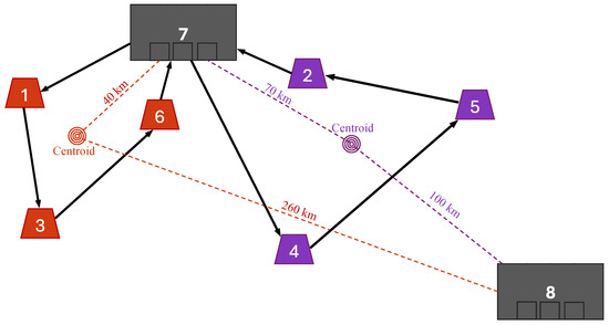
Figure 1.
An example of the centroid of two depots.
5.3. Initial Solution
In the initial solution generation stage, customers, demands, depots, and types of customers are generated based on the data of the instance. Afterwards, the algorithm assigns the sequences, random key values, and depot openings in a pseudo-random manner with the Mersenne Twister MT19937 generator [55]. First, it evaluates the available sequences to choose one according to the waste of the customer (organic or non-organic). After, considering the types of waste that the customer has, it generates a number for both organic and non-organic waste. Finally, a random number of open depots is generated and selected at random.
5.4. Movement Rules: Three Generations of Neighborhoods
The proposed VNS considers three levels of decision making: route sequence, visit sequence, and depot opening. Operators tailored to each level generate various neighborhood structures. These rules affect customer prioritization and sequencing, providing flexibility in visit scheduling to meet diverse visit type demands and allocate depots to each customer. The movement rules are explained below:
- Route Sequence Level: The exchange operator is used in this level. It consists of choosing two nodes (they must have the same type of waste between organic and not organic), and then their random key values are re-assigned. In Figure 2, nodes one and four were chosen and their values were exchanged. This allows changes to be made to the routes.
 Figure 2. An example of the exchange operator.
 - Visit Sequence Level: The Relocate and Shift operators were adapted. First, they select one customer node and, depending on the type of customer, switch the visit sequence of it (within the available sequences). This change can generate a different visit route for the days where the customer was previously.
- Depot Opening Level: Depending on the number of depots, all possible combinations are established, considering openings from one depot up to the corresponding number. Subsequently, the cost of each combination is evaluated, and the opening scheme (number and location) with the lowest cost is selected.
For those levels, when the instance size is large, it is necessary to adapt the moves to reduce the execution time. In these cases, the procedure consists of generating small changes by creating a fixed number of neighbors (1000 in this work) that are random and without repeating selections, allowing the search spaces to be traversed.
5.5. Stopping Criterion
Two types of stopping criteria are established. The first occurs when reaching an execution time limit of 600 s. This value is defined in a general way, based on other algorithms proposed in the literature related to vehicle routing [56,57]. The second occurs when, after a complete iteration, searching among the three neighborhood structures (or decision levels), the algorithm cannot find a solution that improves the current one.
6. Results
This section is divided into three subsections. The first details the adaptation of test cases in which the proposed algorithms were executed, the second validates the use of neighborhood structures in the search, and finally, the computational results are presented.
6.1. Adaptation of the Instances
Since there is no existing database in the literature for the addressed problem with all its characteristics, Cordeau’s library [21] was used as a base and the instances were adapted. This library has 42 instances and has been widely used to validate the Multiple Depot Vehicle Routing Problem and its main variants [49]. The Cordeau’s instances presented the next characteristics: number of vehicles in the closed interval from 1 to 12, customer quantity between 20 and 417, number of planned days from 2 to 10, loading capacity of vehicles, and maximum route duration.
For the new instances, the following main types of waste were identified: organic, plastic, cardboard and paper, glass, metal and WEEE. However, the types of waste are classified as organic and non-organic to simplify the problem. Nodes were generated randomly, taking into account the type of customers, the frequency of visits and their respective feasible day sequences, the demand associated with the type of waste, and location coordinates. The planning horizon is one week of 7 days, during which the collection requirements for both types of waste must be met.
Specifically, evaluating data in the context of recycling in Chile and consulting with experts, the instances were generated considering the following.
- Each depot will have a maximum capacity of 180,000 dm3.
- The number of depots available to open corresponds to of the number of customers.
- Using technical data sheets, it was determined that the capacity of the vehicles should be 18,000 dm3. In relation to the weight capacity, in a variety of Volvo truck brands with this volume, it was found that the standard load capacity is 28,000 kg.
- It was determined that there are 10 vehicles available for each depot that is opened.
- The combination of waste demanded will be assigned to each customer randomly, where each customer will recycle a maximum of three different types of waste out of the five available.
- The amount of waste produced by customers depends on the type of waste they recycle. Likewise, the frequency at which the customer will be visited per week is also assigned (also depending on the type of waste). See Table 5.
Table 5. Demand and frequency parameters based on Chile context.
- In relation to the combination of days available for waste collection, depending on the frequency of each customer, the maximum frequency obtained by type of waste will be chosen [58]. The combination of available days for waste collection will depend on the size of its frequency.
- The demand to be collected from each customer will be the consolidated demand divided by the maximum frequency of visits depending on the types of waste each particular customer has, based on the proposal by [58]. For example, if a customer has organic, paper and cardboard, and glass waste, the maximum frequency that predominates over the others is that of organic waste, with 3 days a week (paper and cardboard have 2 and glass has 1). Thus, the demand is divided by 3 days and the need for collection per visit day is generated. Since metal and WEEE were considered to include electronic waste from appliances and electronic products, it is known that these products contain a small amount of different metals (such as nickel, lead, tin, and mercury) that do not represent a large weight when discarded. In fact, the densest components, which are usually circuit boards, have a density of 1600 kg/m3, but they represent a considerable volume of WEEE. If a vehicle were filled only with WEEE, it should have an average density less than or equal to 1555 kg/m3.
6.2. Validate Neighborhood Structures
In this subsection, the results of executing the proposed algorithm are shown considering each of the three decision levels (Route Sequence Level (RSL), Visit Sequence Level (VSL), and Depot Opening Level (DOL)) independently and comparing them with the algorithm integrating all levels or neighborhood structures. The purpose is to demonstrate that, independently, each level contributes to the search, but by combining the strategies, the synergy among them allows for better results. A total of 15 instances with different sizes (from 23 to 479 nodes) were executed, and 10 replicas were taken for each instance.
Figure 3 shows the average total cost produced (z) for each instance, where Sequence Only, Depot Only, and Random Key Only correspond to the exclusive use of the VSL, DOL, and RSL search levels, respectively. One of the first findings is that depot opening is one of the most influential costs due to its magnitude. On the other hand, when the algorithm uses only RSL or VSL, it maintains the number of depots from the initial solution and improves the routing and sequence assignment of the vehicles. When the algorithm uses only the DOL level, it prefers to open the minimum number of depots but sacrifices transportation costs. Since depot opening cost has the greatest impact on total cost, this level generates the lowest-cost solutions. For the execution of the complete algorithm, it generates solutions with lower total costs than those generated using only one of the decision levels in all sizes. Therefore, the results suggest that the combination of all levels allows for better-performing solutions. Regarding the computational cost for each level, Figure 4 shows the average execution time in each case. The sudden change in time when reaching 276 nodes is because, for these instances, each level performs an exhaustive search of all neighbors; beyond this number of nodes, the search was limited to a maximum of 1000 neighbors.

Figure 3.
Average costs of each level and neighborhood structure.
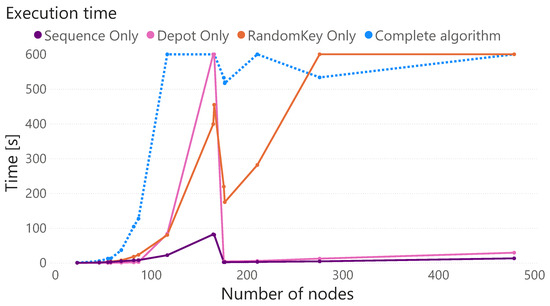
Figure 4.
Average execution times of each level and neighborhood structure.
6.3. Computational Results
The mathematical model and the metaheuristic were carried out on a PC with a GHz GFX AMD Ryzen 5, 3500 U processor and 12 GB of RAM. The proposed mathematical model was executed using CPLEX 22.1.1.0 solver on AMPL language and the metaheuristic was developed on Microsoft Visual Studio using C++ programming language.
The proposed mathematical model did not obtain a feasible solution for any of the instances due to the complexity and size of the instances, with an execution time limit of 600 s. However, the proposed VNS achieved feasible solutions for all instances within the time limit. This comparison does not mean that the mathematical model is flawed; indeed, it was tested with rather small instances and it could find the optimal solutions.
The instances (Inst.) were divided into three groups: small instances, medium-sized instances, and large instances. All tables use the following nomenclature: C: number of customers, D: number of depots, V: number of vehicles available, Z: total cost (USD), St: resolution status (411 for AMPL represents reaching the time limit and finding no solution, and 1 for the proposed VNS represents that could find a feasible solution), t: time (s), d: distance (km). Total cost and distances are expressed in thousands. For the proposed VNS results, a distinction is made between finding a feasible solution and having enough time to return the best solution found. In the first case, it is only verified that the constructive algorithm executed correctly; in the second, it is understood that all search strategies are executed at all decision levels and the stopping criterion is reached.
Table 6 depicts the results for small-sized instances. Here, the size of the problems is between 20 and 60 customers. For all these instances, the algorithm reaches the best solution found using less time than the time limit. Furthermore, the average execution time was s. In all instances of small size, only one depot was opened. The value of z is composed of the transportation cost, dependent on the route, and the opening cost. The latter was set at USD 500,000 for each opened depot.
Table 6.
Small-sized instance results.
Table 7 depicts the results for medium-sized instances. These instances have a considerable number of nodes, increasing the resolution’s complexity. However, the algorithm obtains a feasible solution for all instances and the best solution found for most cases, except for the instances with more than 114 customers, where the execution time limit was reached. In these instances, only one depot was also opened; therefore, the opening cost is set at 500,000 and the average execution time was s.
Table 7.
Medium-sized instance results.
Finally, Table 8 depicts the results for the group of the largest instances; the algorithm reaches the execution time limit for 10 of the 12 instances. It only obtains the best solution found for p12 with 163 customers and p23 with 168 customers. Nonetheless, it obtained a feasible solution for the other instances. Three of the solutions opened two depots (pr06, pr10 and p13) due to capacity constraints; in these cases, the opening cost was and the average time was s.
Table 8.
Large-sized instance results.
Figure 5 shows the summary of the total cost and distance. For instances with more than 300 nodes, the algorithm always opens two depots due to capacity constraints. Consequently, the cost increased by over 1 million, but this allows decreasing the total distance. On the other hand, Figure 6 represents the average execution time for the instances. The global average was s, and for instances larger than 120 nodes, the time increases to 600 s in most cases. In both figures, unusual behavior is observed with the instances of approximately 180 nodes. This is because, despite being of a medium-sized instance, the parameter values (coordinates, demands, etc.) generate a special structure in the constraints that increases the complexity of resolution. Therefore, the costs and computation times are higher.

Figure 5.
Average total cost and distance for the entire algorithm execution.

Figure 6.
Average execution time for the entire algorithm implementation.
Since the mathematical model was unable to solve any evaluated instances, new smaller instances were generated, ranging from 10 to 12 nodes, which are referred to as small-scale instances. These were also adapted from Cordeau’s library [21], and a total of 12 instances were randomly generated. Their results were compared with the proposed VNP. The executions of the mathematical model were performed in Cplex and Gurobi. Table 9 summarizes the results found in the executions, where the letter <a> in the instance names indicates that they are the adapted ones. In all instances, both CPLEX and Gurobi solvers did not find an optimal solution but reported the best solution found within the time limit. The results show that the VNS algorithm not only finds a better objective function compared to the CPLEX and Gurobi solvers but also achieves better results in less time. The difference between the Cplex and Gurobi solvers did not present significant variations in total costs, being favorable to Gurobi by an average of . However, when disaggregating the objective function and only considering transportation costs (since in all cases, a single depot is opened with its associated cost due to the small size of the instances), the difference rises to in favor of Gurobi. On the other hand, the proposed VNS surpasses both solvers within the stipulated time limit, achieving an average improvement of compared to Gurobi for total costs and for the disaggregated cost.
Table 9.
Comparison of results among CPLEX, Gurobi, and the proposed VNS.
7. Limitations and Future Work
Despite the significant contributions presented in this study, several limitations need to be addressed in future research. Firstly, the proposed MILP model and VNS algorithm were tested under specific conditions and assumptions, such as static waste generation rates and fixed traffic conditions. This might limit the applicability of the model in real-world scenarios where waste generation rates can vary dynamically and traffic conditions can change unpredictably. Incorporating real-time data and adaptive mechanisms into the model could enhance its robustness and applicability. Additionally, the model assumes that each type of waste requires exclusive vehicle capacity, which may not be practical or efficient in all contexts.
Secondly, the study primarily focuses on the optimization of logistical costs, including depot establishment, transportation, and operational costs. While these are crucial factors, other important aspects such as the environmental impact of waste collection and recycling operations, customer satisfaction, and the social implications of the waste collection process could be considered. The model can also be expanded to include environmental factors, such as carbon emissions and routing with electric vehicles, which would align with global sustainability goals. Moreover, these extensions would not only improve the model’s ecological impact but also enhance its relevance and applicability in modern logistics.
Thirdly, given the specific characteristics of the problem, no other metaheuristics were found that address the problem in its entirety. Exploring the integration and comparison of other advanced metaheuristic techniques, such as genetic algorithms or ant colony optimization, may offer improvements in solution quality and computational time. Recently, there has also been interest in integrating artificial intelligence tools, such as Reinforcement Learning, with metaheuristics to guide neighborhood search based on data and the learning from past solutions; this could be an opportunity to further improve the search.
8. Conclusions
The constant population growth, increased demand for products in emerging economies, and global warming have significantly increased the consumption of goods, resulting in large amounts of waste in both businesses and households. This has highlighted the need to develop more efficient collection systems to mitigate negative effects in cities. This paper addresses the Periodic Location Routing Problem (PLRP) with multiple depots. This logistic problem integrates the location of distribution centers, vehicle route planning, and periodic delivery scheduling to meet customer demands. An important feature is the integration of a periodic time horizon into the problem (e.g., weeks). The objective is to minimize total costs, including depot establishment costs, transportation costs, and operational costs, ensuring that each customer is served with the required frequency. This paper considers a selective recycling context involving major waste materials: organic, plastic, paper and cardboard, glass, and waste from electrical and electronic equipment (WEEE). This inclusion introduces new decision levels, as customers may have multiple types of waste, different recycling needs, and feasible visit frequencies that can also vary among customers. Additionally, the vehicles collecting the waste must have the exclusive capacity for each type of recycling.
To solve this problem, a mathematical model based on mixed-integer linear programming was designed to minimize logistic costs, including depot opening costs and vehicle kilometer costs. To validate the model, Cordeau’s library was adapted to the problem’s context and the parameters of a case were applied in Chile. A total of 42 instances of various sizes were generated: small (20 to 60 customers), medium (72 to 144 customers), and large (153 to 417 customers). The results of the mathematical model showed that it not only failed to reach an optimal value within a time limit of 10 min for any instance size but also failed to find a feasible solution. Therefore, a metaheuristic based on Variable Neighborhood Search (VNS) was designed with three neighborhood structures focused on each decision level: Route Sequence Level, Visit Sequence Level, and Depot Opening Level. The first corresponds to the routing sequence of each vehicle, the second explores the possible feasible combinations of days for recycling for each customer, and the third evaluates the number of necessary depots. The results show that the VNS outperformed the mathematical model in terms of time and solution quality in all cases. It was also demonstrated that the combination of the three neighborhood structures improved the performance of each individually, despite the creation of neighborhoods being limited to exploring 1000 neighbors for large instance cases. Finally, smaller test instances were generated to validate the proposed mathematical model with different solvers (CPLEX and Gurobi) and the proposed VNS. The results show that although feasible solutions were found with both solvers, the VNS outperformed them by concerning the disaggregated objective function value (only transportation costs, since a depot was always opened).
In conclusion, the proposed Mixed-Integer Linear Programming (MILP) model and the Variable Neighborhood Search (VNS) metaheuristic present significant advancements in solving the Periodic Location Routing Problem (PLRP) for urban waste collection. Unlike traditional methods, our approach characterizes 25 distinct customer types based on heterogeneous waste demands and visit frequencies, ensuring tailored and efficient waste management. The integration of selective recycling needs, combined with a three-level decision-making structure (Route Sequence, Visit Sequence, and Depot Opening), provides a comprehensive and practical solution. Computational experiments demonstrate the VNS algorithm’s superiority, delivering solutions seven times better than exact methods in a fraction of the time and achieving feasible results where the MILP model fails. This work not only enhances logistical efficiency but also aligns with global sustainability goals by promoting effective waste separation and recycling. The proposed model and metaheuristic are based on real-world data and assumptions pertinent to the Chilean context. The customer types, visit frequencies, waste demands, and vehicle capacities were all derived from actual Chilean data. For instance, cost per distance was specifically considered, acknowledging Santiago de Chile’s relatively flat terrain, which lacks pronounced slopes. Therefore, the transportation cost largely depends on the Euclidean distance. These localized parameters ensure that the model reflects the practical realities of waste management in Chile. Given these considerations, the proposed model is feasible for implementation by relevant Chilean authorities. Its design aligns with the geographical and operational characteristics of Chile, offering a tailored solution that can effectively address the country’s urban waste management challenges.
Author Contributions
Conceptualization, D.M.-T. and G.G.; Methodology, D.N.-Z. and J.C.R.-V.; Software, D.N.-Z., J.C.R.-V. and D.M.-T.; Formal analysis, G.G.; Investigation, D.N.-Z. and J.C.R.-V.; Data curation, D.N.-Z., J.C.R.-V. and G.G.; Writing—original draft, D.N.-Z. and J.C.R.-V.; Writing—review and editing, D.M.-T.; supervision and project administration, D.M.-T. and G.G. All authors have read and agreed to the published version of the manuscript.
Funding
This research received no external funding.
Data Availability Statement
The original contributions presented in the study are included in the article, and all data were published in the following repository: https://github.com/dmorill/PLRP_instances accessed on 8 July 2024, for any additional questions about methodology or the source code, please contact the corresponding author.
Conflicts of Interest
The authors declare no conflicts of interest.
References
- OECD. Plastic Pollution Is Growing Relentlessly as Waste Management and Recycling Fall Short, Says OECD; OECD: Paris, France, 2022. [Google Scholar]
- Ramos, T.R.P.; Gomes, M.I.; Barbosa-Póvoa, A.P. Economic and environmental concerns in planning recyclable waste collection systems. Transp. Res. Part E Logist. Transp. Rev. 2014, 62, 34–54. [Google Scholar] [CrossRef]
- Gruler, A.; Juan, A.A.; Contreras-Bolton, C.; Gatica, G. A Biased-Randomized Heuristic for the Waste Collection Problem in Smart Cities. Adv. Intell. Syst. Comput. 2018, 730, 255–263. [Google Scholar] [CrossRef]
- Senior, K.; Mazza, A. Italian “Triangle of death” linked to waste crisis. Lancet Oncol. 2004, 5, 525–527. [Google Scholar] [CrossRef] [PubMed]
- United Nations. Sustainable Development Goals—Goal 12: Ensure Sustainable Consumption and Production Patterns; United Nations: New York, NY, USA, 2023. [Google Scholar]
- Boskovic, G.; Jovicic, N.; Jovanovic, S.; Simovic, V. Calculating the costs of waste collection: A methodological proposal. Waste Manag. Res. J. Sustain. Circ. Econ. 2016, 34, 775–783. [Google Scholar] [CrossRef] [PubMed]
- Eksioglu, B.; Vural, A.V.; Reisman, A. The vehicle routing problem: A taxonomic review. Comput. Ind. Eng. 2009, 57, 1472–1483. [Google Scholar] [CrossRef]
- Ouertani, N.; Ben-Romdhane, H.; Nouaouri, I.; Allaoui, H.; Krichen, S. A multi-compartment VRP model for the health care waste transportation problem. J. Comput. Sci. 2023, 72, 102104. [Google Scholar] [CrossRef]
- Mojtahedi, M.; Fathollahi-Fard, A.M.; Tavakkoli-Moghaddam, R.; Newton, S. Sustainable vehicle routing problem for coordinated solid waste management. J. Ind. Inf. Integr. 2021, 23, 100220. [Google Scholar] [CrossRef]
- Mohammadi, M.; Rahmanifar, G.; Hajiaghaei-Keshteli, M.; Fusco, G.; Colombaroni, C.; Sherafat, A. A dynamic approach for the multi-compartment vehicle routing problem in waste management. Renew. Sustain. Energy Rev. 2023, 184, 113526. [Google Scholar] [CrossRef]
- Eren, E.; Rıfat Tuzkaya, U. Safe distance-based vehicle routing problem: Medical waste collection case study in COVID-19 pandemic. Comput. Ind. Eng. 2021, 157, 107328. [Google Scholar] [CrossRef]
- Prodhon, C. A Metaheuristic for the Periodic Location-Routing Problem. Oper. Res. Proc. 2008, 2007, 159–164. [Google Scholar] [CrossRef]
- Rabbani, M.; Amirhossein Sadati, S.; Farrokhi-Asl, H. Incorporating location routing model and decision making techniques in industrial waste management: Application in the automotive industry. Comput. Ind. Eng. 2020, 148, 106692. [Google Scholar] [CrossRef]
- Prodhon, C. A hybrid evolutionary algorithm for the periodic location-routing problem. Eur. J. Oper. Res. 2011, 210, 204–212. [Google Scholar] [CrossRef]
- Ahmadi Basir, S.; Şahin, G.; Özbaygın, G. A comparative study of alternative formulations for the periodic vehicle routing problem. Comput. Oper. Res. 2024, 165, 106583. [Google Scholar] [CrossRef]
- Hemmelmayr, V.; Smilowitz, K.; de la Torre, L. A periodic location routing problem for collaborative recycling. IISE Trans. 2017, 49, 414–428. [Google Scholar] [CrossRef]
- Dantzig, G.B.; Ramser, J.H. The Truck Dispatching Problem. Manag. Sci. 1959, 6, 80–91. [Google Scholar] [CrossRef]
- Campbell, A.M.; Wilson, J.H. Forty years of periodic vehicle routing. Networks 2014, 63, 2–15. [Google Scholar] [CrossRef]
- Beltrami, E.J.; Bodin, L.D. Networks and vehicle routing for municipal waste collection. Networks 1974, 4, 65–94. [Google Scholar] [CrossRef]
- Christofides, N.; Beasley, J.E. The period routing problem. Networks 1984, 14, 237–256. [Google Scholar] [CrossRef]
- Cordeau, J.F.; Gendreau, M.; Laporte, G. A tabu search heuristic for periodic and multi-depot vehicle routing problems. Networks 1997, 30, 105–119. [Google Scholar] [CrossRef]
- Salhi, S.; Thangiah, S.R.; Rahman, F. A Genetic Clustering Method for the Multi-Depot Vehicle Routing Problem. In Artificial Neural Nets and Genetic Algorithms; Springer: Vienna, Austria, 1998; pp. 234–237. [Google Scholar] [CrossRef]
- Drummond, L.M.; Ochi, L.S.; Vianna, D.S. An asynchronous parallel metaheuristic for the period vehicle routing problem. Future Gener. Comput. Syst. 2001, 17, 379–386. [Google Scholar] [CrossRef]
- Teixeira, J.; Antunes, A.P.; de Sousa, J.P. Recyclable waste collection planning—A case study. Eur. J. Oper. Res. 2004, 158, 543–554. [Google Scholar] [CrossRef]
- Irnich, S.; Toth, P.; Vigo, D. Chapter 1: The Family of Vehicle Routing Problems. In Vehicle Routing; Society for Industrial and Applied Mathematics: Philadelphia, PA, USA, 2014; pp. 1–33. [Google Scholar] [CrossRef]
- Prodhon, C. An ELSxPath Relinking Hybrid for the Periodic Location-Routing Problem. Hybrid Metaheuristics 2009, 5818, 15–29. [Google Scholar] [CrossRef]
- Pirkwieser, S.; Raidl, G.R. Variable Neighborhood Search Coupled with ILP-Based Very Large Neighborhood Searches for the (Periodic) Location-Routing Problem. Hybrid Metaheuristics 2010, 6373, 174–189. [Google Scholar] [CrossRef]
- Vidal, T.; Crainic, T.G.; Gendreau, M.; Lahrichi, N.; Rei, W. A Hybrid Genetic Algorithm for Multidepot and Periodic Vehicle Routing Problems. Oper. Res. 2012, 60, 611–624. [Google Scholar] [CrossRef]
- Hemmelmayr, V.C. Sequential and parallel large neighborhood search algorithms for the periodic location routing problem. Eur. J. Oper. Res. 2015, 243, 52–60. [Google Scholar] [CrossRef]
- Koç, Ç. A unified-adaptive large neighborhood search metaheuristic for periodic location-routing problems. Transp. Res. Part C Emerg. Technol. 2016, 68, 265–284. [Google Scholar] [CrossRef]
- Yu, Y.; Wang, S.; Wang, J.; Huang, M. A branch-and-price algorithm for the heterogeneous fleet green vehicle routing problem with time windows. Transp. Res. Part B Methodol. 2019, 122, 511–527. [Google Scholar] [CrossRef]
- Aringhieri, R.; Bruglieri, M.; Malucelli, F.; Nonato, M. A Special Vehicle Routing Problem Arising in the Optimization of Waste Disposal: A Real Case. Transp. Sci. 2018, 52, 277–299. [Google Scholar] [CrossRef]
- Franca, L.S.; Ribeiro, G.M.; Chaves, G.d.L.D. The planning of selective collection in a real-life vehicle routing problem: A case in Rio de Janeiro. Sustain. Cities Soc. 2019, 47, 101488. [Google Scholar] [CrossRef]
- Flores-Carrasco, J.; Morillo-Torres, D.; Escobar, J.; Linfati, R.; Gatica, G. The Periodic Location-Routing with Selective Recycling Problem: Two Solution Approaches. IFAC-PapersOnLine 2021, 54, 787–792. [Google Scholar] [CrossRef]
- Vidović, M.; Ratković, B.; Bjelić, N.; Popović, D. A two-echelon location-routing model for designing recycling logistics networks with profit: MILP and heuristic approach. Expert Syst. Appl. 2016, 51, 34–48. [Google Scholar] [CrossRef]
- Wang, L.; Zhao, X.; Wu, P. Resource-Constrained Emergency Scheduling for Forest Fires via Artificial Bee Colony and Variable Neighborhood Search Combined Algorithm. IEEE Trans. Intell. Transp. Syst. 2024, 25, 5791–5806. [Google Scholar] [CrossRef]
- Meng, L.; Cheng, W.; Zhang, B.; Zou, W.; Duan, P. A novel hybrid algorithm of genetic algorithm, variable neighborhood search and constraint programming for distributed flexible job shop scheduling problem. Int. J. Ind. Eng. Comput. 2024, 15, 813–832. [Google Scholar] [CrossRef]
- García-Vasquez, K.; Linfati, R.; Escobar, J.W. A three-phase algorithm for the pollution traveling Salesman problem. Heliyon 2024, 10. [Google Scholar] [CrossRef] [PubMed]
- Ferreira, K.; de Queiroz, T.; Munari, P.; Toledo, F. A variable neighborhood search for the green vehicle routing problem with two-dimensional loading constraints and split delivery. Eur. J. Oper. Res. 2024, 316, 597–616. [Google Scholar] [CrossRef]
- İslim, R.B.; Çatay, B. An effective matheuristic approach for solving the electric traveling salesperson problem with time windows and battery degradation. Eng. Appl. Artif. Intell. 2024, 132, 107943. [Google Scholar] [CrossRef]
- Su, Y.; Zhang, S.; Zhang, C. A lightweight genetic algorithm with variable neighborhood search for multi-depot vehicle routing problem with time windows. Appl. Soft Comput. 2024, 161, 111789. [Google Scholar] [CrossRef]
- Lou, P.; Zhou, Z.; Zeng, Y.; Fan, C. Vehicle routing problem with time windows and carbon emissions: A case study in logistics distribution. Environ. Sci. Pollut. Res. 2024, 31, 41600–41620. [Google Scholar] [CrossRef] [PubMed]
- Prakash, R.; Pushkar, S. Green vehicle routing problem: Metaheuristic solution with time window. Expert Syst. 2024, 41, e13007. [Google Scholar] [CrossRef]
- Chagas, G.O.; Lorena, L.A.; dos Santos, R.D.; Renaud, J.; Coelho, L.C. A parallel variable neighborhood search for α-neighbor facility location problems. Comput. Oper. Res. 2024, 165, 106589. [Google Scholar] [CrossRef]
- Wei, C.; Wøhlk, S.; Che, A. A multi-level capacitated arc routing problem with intermediate facilities in waste collection. Comput. Oper. Res. 2024, 167, 106671. [Google Scholar] [CrossRef]
- Peng, Z.; Li, Y.; Zhang, J. Joint optimization of train timetable and passing facility: A capacity allocation strategy. Expert Syst. Appl. 2024, 252, 124173. [Google Scholar] [CrossRef]
- Souza, V.A.; Melo, R.A.; Mateus, G.R. The Vehicle Routing Problem with Cross-Docking and Scheduling at the Docking Station: Compact formulation and a General Variable Neighborhood Search metaheuristic. Appl. Soft Comput. 2024, 161, 111744. [Google Scholar] [CrossRef]
- Sugianto, W.C.; Kim, B.S. Iterated variable neighborhood search for integrated scheduling of additive manufacturing and multi-trip vehicle routing problem. Comput. Oper. Res. 2024, 167, 106659. [Google Scholar] [CrossRef]
- Hemmelmayr, V.C.; Doerner, K.F.; Hartl, R.F. A variable neighborhood search heuristic for periodic routing problems. Eur. J. Oper. Res. 2009, 195, 791–802. [Google Scholar] [CrossRef]
- Voigt, S.; Frank, M.; Fontaine, P.; Kuhn, H. Hybrid adaptive large neighborhood search for vehicle routing problems with depot location decisions. Comput. Oper. Res. 2022, 146, 105856. [Google Scholar] [CrossRef]
- Sluijk, N.; Florio, A.M.; Kinable, J.; Dellaert, N.; Van Woensel, T. Two-echelon vehicle routing problems: A literature review. Eur. J. Oper. Res. 2023, 304, 865–886. [Google Scholar] [CrossRef]
- Wang, K.; Shao, Y.; Zhou, W. Matheuristic for a two-echelon capacitated vehicle routing problem with environmental considerations in city logistics service. Transp. Res. Part D Transp. Environ. 2017, 57, 262–276. [Google Scholar] [CrossRef]
- de Melo, V.A.; Boaventura-Netto, P.O. Metaheuristics Evaluation: A Proposal for A Multicriteria Methodology. Pesqui. Oper. 2015, 35, 539–554. [Google Scholar] [CrossRef]
- Mladenović, N.; Hansen, P. Variable neighborhood search. Comput. Oper. Res. 1997, 24, 1097–1100. [Google Scholar] [CrossRef]
- Matsumoto, M.; Nishimura, T. Mersenne twister: A 623-dimensionally equidistributed uniform pseudo-random number generator. ACM Trans. Model. Comput. Simul. 1998, 8, 3–30. [Google Scholar] [CrossRef]
- Sarasola, B.; Doerner, K.F. Adaptive large neighborhood search for the vehicle routing problem with synchronization constraints at the delivery location. Networks 2020, 75, 64–85. [Google Scholar] [CrossRef]
- Alvarez, A.; Munari, P. An exact hybrid method for the vehicle routing problem with time windows and multiple deliverymen. Comput. Oper. Res. 2017, 83, 1–12. [Google Scholar] [CrossRef]
- Prodhon, C.; Prins, C. A Memetic Algorithm with Population Management (MA|PM) for the Periodic Location-Routing Problem. Hybrid Metaheuristics 2008, 5296, 43–57. [Google Scholar] [CrossRef]


Disclaimer/Publisher’s Note: The statements, opinions and data contained in all publications are solely those of the individual author(s) and contributor(s) and not of MDPI and/or the editor(s). MDPI and/or the editor(s) disclaim responsibility for any injury to people or property resulting from any ideas, methods, instructions or products referred to in the content. |
© 2024 by the authors. Licensee MDPI, Basel, Switzerland. This article is an open access article distributed under the terms and conditions of the Creative Commons Attribution (CC BY) license (https://creativecommons.org/licenses/by/4.0/).