
Novel Landfill-Gas-to-Biomethane Route Using a Gas–Liquid Membrane Contactor for Decarbonation/Desulfurization and Selexol Absorption for Siloxane Removal


Abstract
:1. Introduction
1.1. Landfill-Gas Decarbonation: Advantages of Gas–Liquid Membrane Contactors
1.2. GLMC Modeling for Landfill-Gas/Biogas Decarbonation
1.3. GLMC Modeling in Process Simulators
1.4. Siloxane Removal from Landfill-Gas: The Advantages of Selexol Absorption
1.5. The Present Work
2. Methods
2.1. GLMC-UOE Development
2.1.1. Element Mass Balances
2.1.2. Element Energy Balances
2.1.3. Element Pressure Drop
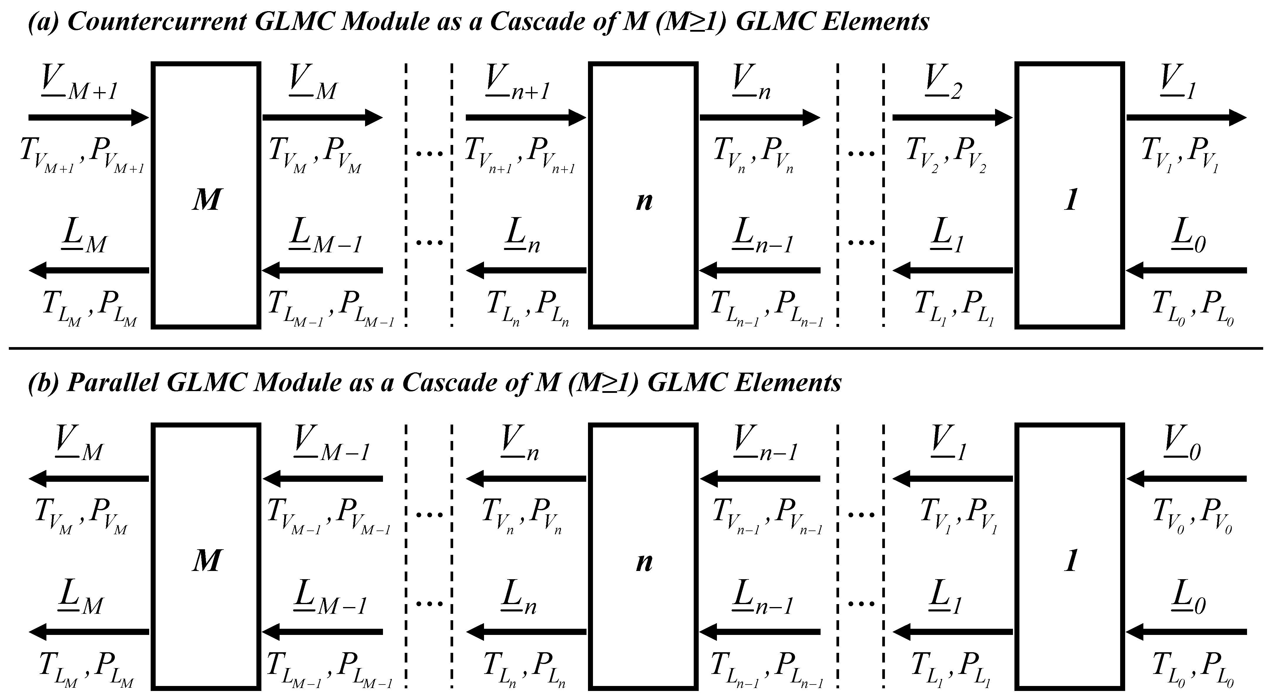
2.1.4. Algorithm to Solve the Countercurrent GLMC Model (GLMC-CCC-D)
2.1.5. Algorithm to Solve the Parallel-Contact GLMC (GLMC-PC-D)
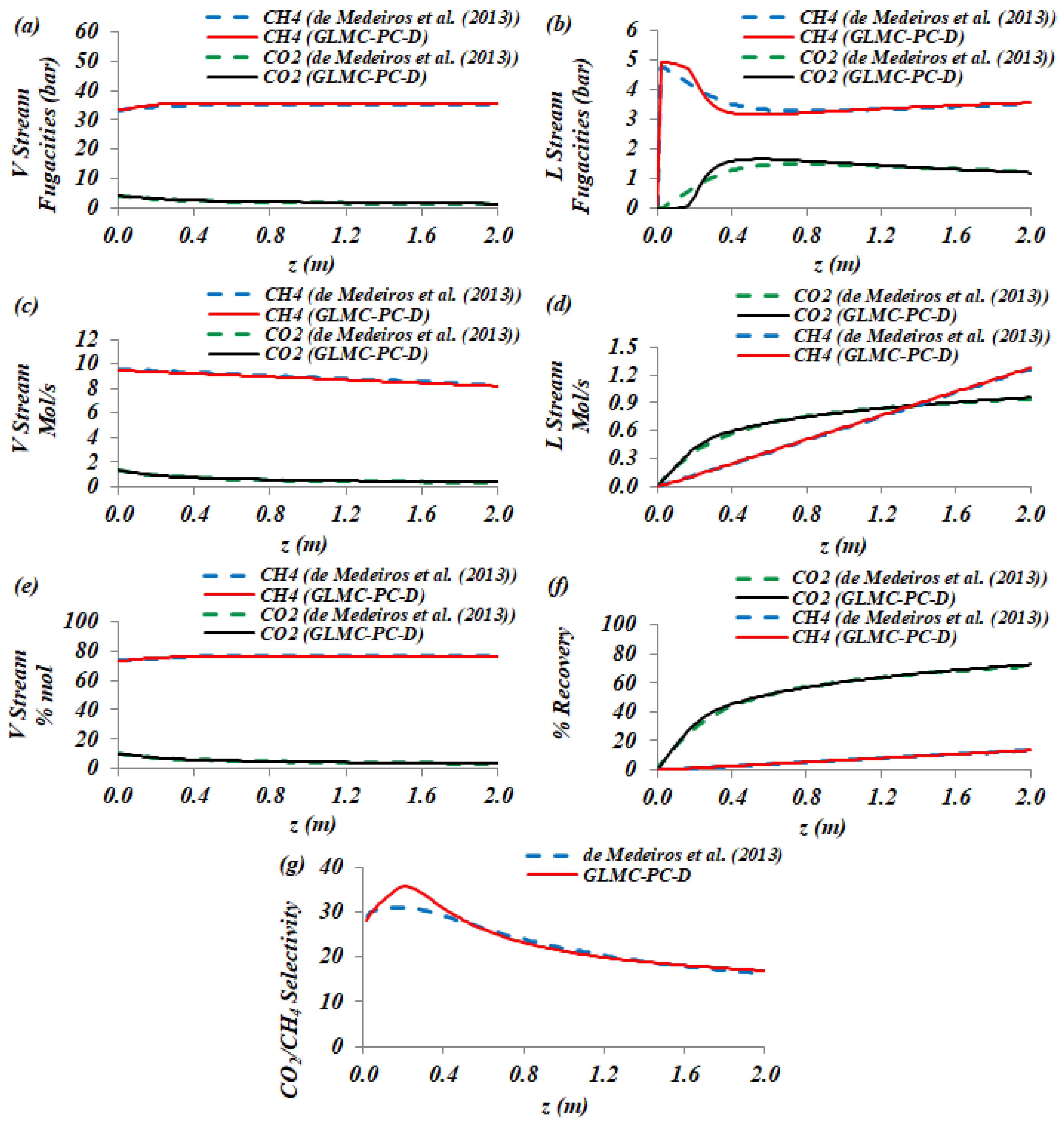
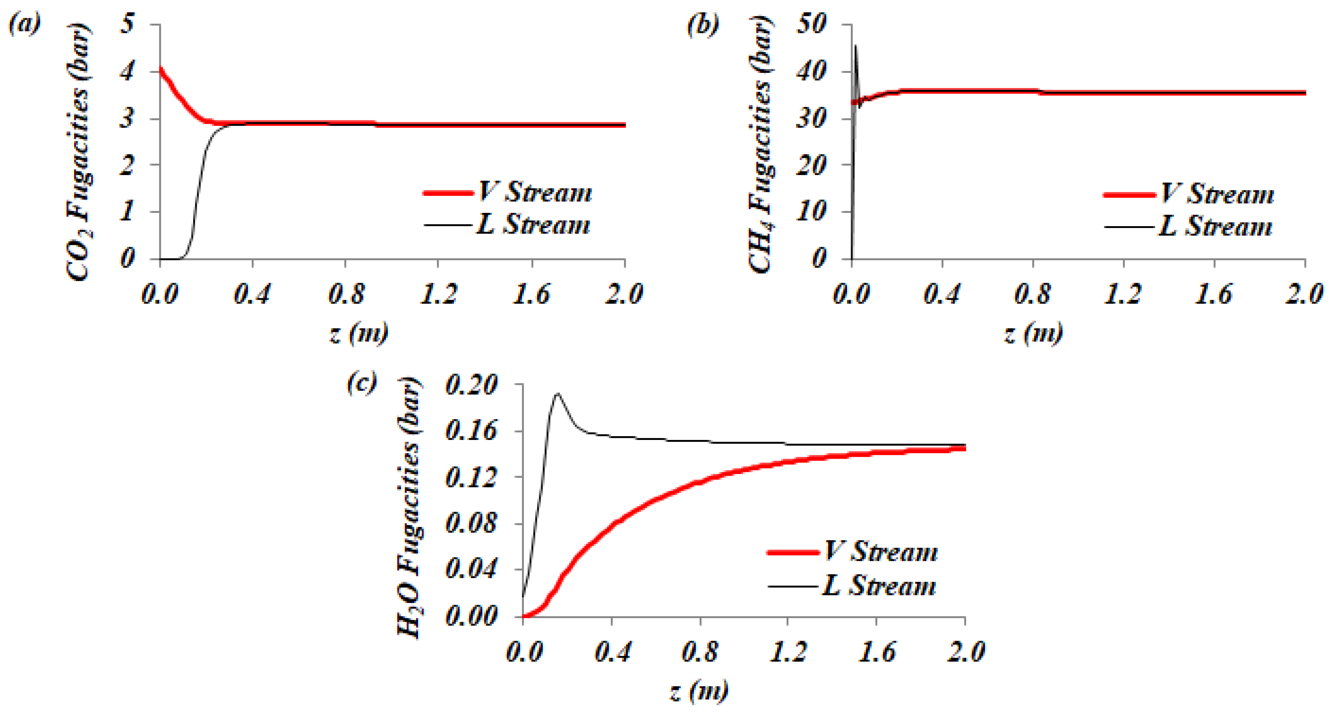
2.1.6. GLMC-UOE Validation
2.2. Landfill-Gas Composition
2.3. Landfill-Gas-to-Biomethane Simulation Assumptions
2.4. Landfill-Gas-to-Biomethane Process
2.4.1. Landfill-Gas Pre-Processing and Compression
2.4.2. Intensified GLMC Decarbonation/Desulfurization with Pressurized Water
2.4.3. Siloxane Removal via DEPG Absorption
3. Landfill-Gas-to-Biomethane Process: Results and Discussion
3.1. Landfill-Gas Decarbonation/Desulfurization Results
3.2. Siloxane Separation, Process Waste, and Power/Utilities Consumption
4. Conclusions
Supplementary Materials
Author Contributions
Funding
Data Availability Statement
Conflicts of Interest
Abbreviations
Nomenclature
| HFM-side and shell-side flow-section areas (m2) | |
| GLMC module transfer area (m2) | |
| , | Shell internal diameter, HFM-side hydraulic diamter, and shell-side hydraulic diameter (m) |
| Internal/external HFM diameters (m) | |
| L/V species k fugacities at element n (bar) | |
| Logarithmic mean of k transmembrane fugacity difference at element n (bar) | |
| L/V kth partial molar enthalpies at element n (kJ/kmol) | |
| L/V molar enthalpies at element n (kJ/kmol) | |
| Shell-side and HFM-side head losses for element n (Pa) | |
| Vector of species L molar flowrates leaving element n (mol/s) | |
| Number of discretized GLMC elements; number of HFMs per module | |
| Transmembrane k transfer rate (mol/s) in element n and number of modules | |
| Cente–-center distance of adjacent HFMs (m) | |
| L/V pressures of element n (bar) | |
| Logarithmic mean transmembrane temperature difference at element n (K) | |
| L/V temperatures of element n (K) | |
| External/internal GLMC heat transfer coefficients (kJ/(h.m2.K)) | |
| Vector of species V molar flowrates leaving element n (mol/s) | |
| L/V axial velocities at element n (m/s) | |
| L and V species k mol fraction | |
| , z | GLMC length; GLMC axial position (m) |
| Greek Symbols | |
| Packing ratio; Kozeny factor | |
| L/V dynamic viscosities at element n (Pa.s) | |
| Transmembrane k mass transfer coefficient (mol/(s.bar.m2)) | |
| L/V molar densities at element n (kmol/m3) |
Appendix A. GLMC-PC-D Model Validation

| Item | Value | Item | Value | Item | Value | Item | Value |
|---|---|---|---|---|---|---|---|
| 0.8 m | 0.502 mm | mol/(s.bar.m2) | mol/(s.bar.m2) | ||||
| 2 m | mol/(s.bar.m2) | mol/(s.bar.m2) | |||||
| Volume | 1.005 m3 | 6901.4 m2 | mol/(s.bar.m2) | mol/(s.bar.m2) | |||
| 40 | 27 °C | mol/(s.bar.m2) | mol/(s.bar.m2) | ||||
| 0.5 mm | 5 W/(m2.K) | mol/(s.bar.m2) | 2 W/(m2.K) |
| Solvent Inlet | CO2-Rich NG Inlet | Treated Gas [54] | Treated-Gas GLMC-PC-D | |
|---|---|---|---|---|
| P (bar) | 5.0 | 50.0 | 49.85 | 49.85 |
| T (°C) | 26.85 | 26.85 | 38.80 | 39.77 |
| MMNm3/d | - | 1.0 | 0.830 | 0.829 |
| kg/h | 17,651 | - | - | - |
| CO2 (%mol) | 0 | 10.19 | 3.50 | 3.36 |
| CH4 (%mol) | 0 | 73.22 | 76.5 | 76.41 |
| C2H6 (%mol) | 0 | 9.09 | 11.00 | 10.97 |
| C3H8 (%mol) | 0 | 4.25 | 5.10 | 5.14 |
| C4H10 (%mol) | 0 | 1.78 | 2.20 | 2.15 |
| C5H12 (%mol) | 0 | 1.47 | 1.80 | 1.77 |
| H2O (%mol) | 60 | 0 | 0 | 0.20 |
| MEA (%mol) | 20 | 0 | 0 | |
| MDEA (%mol) | 20 | 0 | 0 |
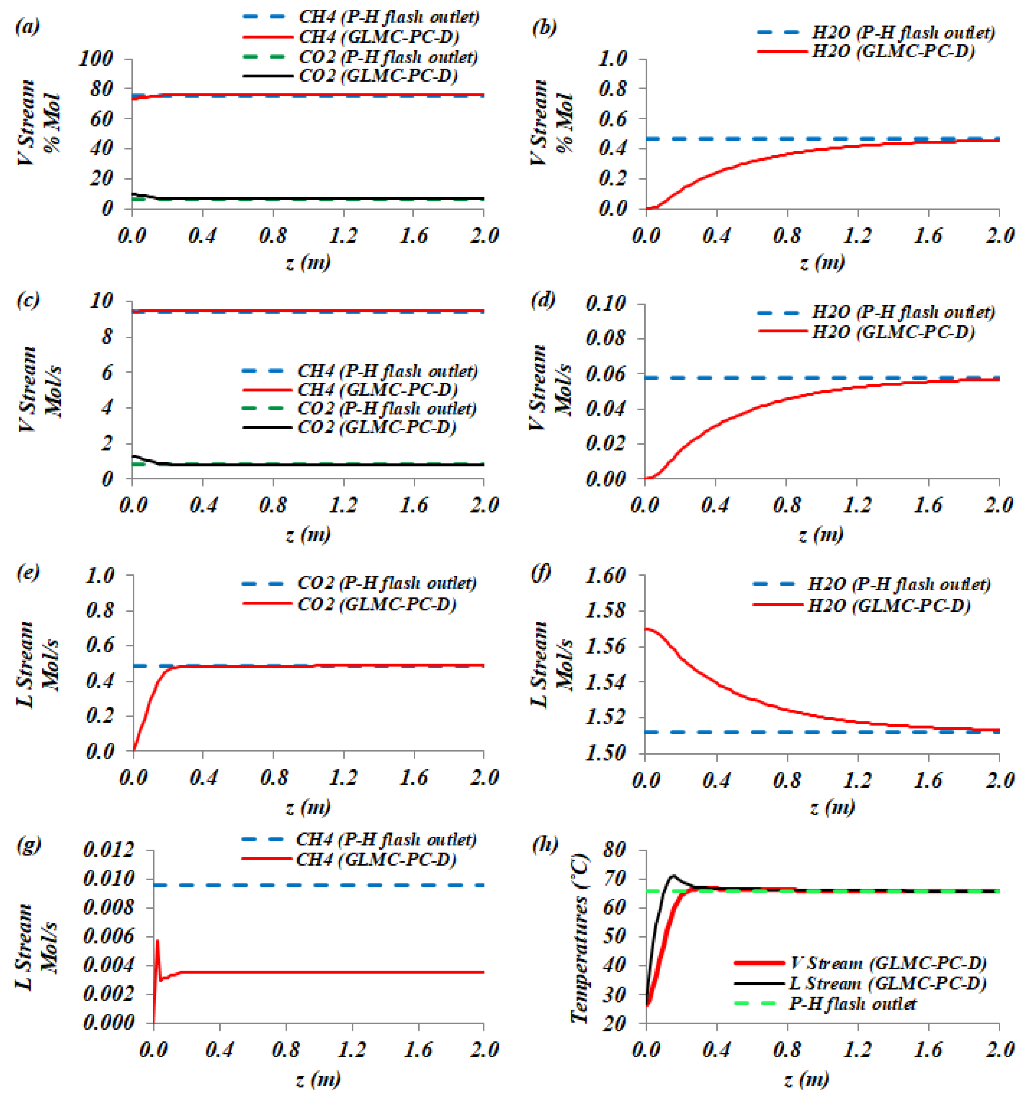
Appendix B. GLMC-PC-D Model Asymptotic Validation with P-H Flash
| CO2-Rich Solvent P-H Flash | CO2-Rich Solvent GLMC-PC-D | Treated-Gas P-H Flash | Treated-Gas GLMC-PC-D | |
|---|---|---|---|---|
| P (bar) | 50.0 | 50.0 | 50.0 | 50.0 |
| T (°C) | 65.90 | 65.90 | 65.90 | 65.90 |
| kmol/h | 440.4 | 439.3 | 1796.4 | 1797.5 |
| kg/h | 20,629 | 20,605 | 39,302 | 39,326 |
| CO2 (%mol) | 15.94 | 15.99 | 6.64 | 6.64 |
| CH4 (%mol) | 0.31 | 0.12 | 75.74 | 75.74 |
| C2H6 (%mol) | 0.06 | 0.01 | 9.40 | 9.40 |
| C3H8 (%mol) | 0.02 | 4.40 | 4.40 | |
| C4H10 (%mol) | 0.01 | 1.52 | 1.52 | |
| C5H12 (%mol) | 0.01 | 1.84 | 1.84 | |
| H2O (%mol) | 49.43 | 49.58 | 0.46 | 0.46 |
| MEA (%mol) | 17.11 | 17.15 | ||
| MDEA (%mol) | 17.11 | 17.15 |
Appendix C. GLMC-CCC-D Asymptotic Validation with an Adiabatic Absorption Column
| Item | CO2-Rich Solvent Absorber | CO2-Rich Solvent GLMC-CCC-D | Treated-Gas Absorber | Treated-Gas GLMC-CCC-D |
|---|---|---|---|---|
| P (bar) | 50.0 | 50.0 | 50.0 | 50.0 |
| T (°C) | 26.53 | 40.12 | 91.75 | 89.87 |
| kmol/h | 444.0 | 456.9 | 1792.8 | 1779.9 |
| kg/h | 21,182 | 21,185 | 38,749 | 38,746 |
| CO2 (%mol) | 20.09 | 17.59 | 5.60 | 6.13 |
| CH4 (%mol) | 0.11 | 0.11 | 75.93 | 76.48 |
| C2H6 (%mol) | 0.04 | 9.42 | 9.50 | |
| C3H8 (%mol) | 0.02 | 4.41 | 4.44 | |
| C4H10 (%mol) | 0.01 | 1.52 | 1.54 | |
| C5H12 (%mol) | 0.01 | 1.86 | 1.86 | |
| H2O (%mol) | 45.81 | 49.32 | 1.26 | 0.05 |
| MEA (%mol) | 16.95 | 16.49 | ||
| MDEA (%mol) | 16.96 | 16.49 |
Appendix D. GLMC-CCC-D Model Validation: Water Solvent GLMC

| Biomethane [47] | Biomethane GLMC-CCC-D | Off Gas [47] | Off-Gas GLMC-CCC-D | |
|---|---|---|---|---|
| P (bar) | -- | 7.996 | -- | 0.6831 |
| T (°C) | 15 | 15.25 | 15 | 18.37 |
| Nm3/h | 33.61 | 33.73 | 140.88 | 141.55 |
| CO2 (%mol) | 2 | 2 | 13.4 | 13.7 |
| CH4 (%mol) | 98 | 98 | 2.2 | 2.2 |
| N2 (%mol) | 0 | 0 | 84.3 | 84.1 |
| Process: General Results | ||||
| Belaissaoui and Favre [47] | GLMC-CCC-D | |||
| Liquid Pressure Drop (bar) | 2.43 | 2.47 | ||
| CO2 %Removal | 96.65 | 96.53 | ||
| CH4 %Loss | 8.7 | 8.5 | ||
| CO2-Rich Solvent Temperature (°C) | 15 | 15.26 | ||
| Regenerated Solvent Temperature (°C) | 15 | 15.03 | ||
Appendix E. GLMC Internal Heat Transfer Coefficient for Landfill-Gas Purification
| Item | CO2-Rich Water Absorber | CO2-Rich Water GLMC-CCC-D | Treated-Gas Absorber | Treated-Gas GLMC-CCC-D |
|---|---|---|---|---|
| P (bar) | 7.1 | 6.664 | 7.0 | 6.998 |
| T (°C) | 15.37 | 15.37 | 15.02 | 15.08 |
| MMNm3/d | - | - | 0.252957 | 0.253672 |
| kg/h | 7,276,541 | 7,276,586 | - | - |
| CH4 (%mol) | 0.01 | 0.01 | 99.10 | 99.10 |
| CO2 (%mol) | 0.09 | 0.09 | 0.64 | 0.13 |
| H2S (ppm-mol) | ||||
| H2O (%mol) | 99.90 | 99.90 | 0.26 | 0.26 |
References
- Popov, V. A new landfill system for cheaper landfill gas purification. Renew. Energy 2005, 30, 1021–1029. [Google Scholar] [CrossRef]
- Yang, L.; Ge, X.; Wan, C.; Yu, F.; Li, Y. Progress and perspectives in converting biogas to transportation fuels. Renew. Sustain. Energy Rev. 2014, 40, 1133–1152. [Google Scholar] [CrossRef]
- Zhou, K.; Chaemchuen, S.; Verpoort, F. Alternative materials in technologies for biogas upgrading via CO2 capture. Renew. Sustain. Energy Rev. 2017, 79, 1414–1441. [Google Scholar] [CrossRef]
- Wise, D.L.; Kispert, R.G.; Langton, E.W. A review of bioconversion systems for energy recovery from municipal solid waste part II: Fuel gas production. Resour. Conserv. 1981, 6, 117–136. [Google Scholar] [CrossRef]
- Parker, N.; Williams, R.; Dominguez-Faus, R.; Scheitrum, D. Renewable natural gas in California: An assessment of the technical and economic potential. Energy Policy 2017, 111, 235–245. [Google Scholar] [CrossRef]
- Nadaletti, W.C.; Cremonez, P.A.; de Souza, S.N.M.; Bariccatti, R.A.; Belli Filho, P.; Secco, D. Potential use of landfill biogas in urban bus fleet in the Brazilian states: A review. Renew. Sustain. Energy Rev. 2015, 41, 277–283. [Google Scholar] [CrossRef]
- Keogh, N.; Corr, D.; Monaghan, R.F.D. Biogenic renewable gas injection into natural gas grids: A review of technical and economic modelling studies. Renew. Sustain. Energy Rev. 2022, 168, 112818. [Google Scholar] [CrossRef]
- Schipfer, F.; Mäki, E.; Schmieder, U.; Lange, N.; Schildhauer, T.; Hennig, C.; Thrän, D. Status of and expectations for flexible bioenergy to support resource efficiency and to accelerate the energy transition. Renew. Sustain. Energy Rev. 2022, 158, 112094. [Google Scholar] [CrossRef]
- Araújo, O.Q.F.; de Medeiros, J.L. How is the transition away from fossil fuels doing, and how will the low-carbon future unfold? Clean Technol. Environ. Policy 2021, 23, 1385–1388. [Google Scholar] [CrossRef]
- Araújo, O.Q.F.; Boa Morte, I.B.; Borges, C.L.T.; Morgado, C.R.V.; de Medeiros, J.L. Beyond clean and affordable transition pathways: A review of issues and strategies to sustainable energy supply. Int. J. Electr. Power Energy Syst. 2024, 155, 109544. [Google Scholar] [CrossRef]
- Yu, H.; Xu, H.; Fan, J.; Zhu, Y.B.; Wang, F.; Wu, H. Transport of shale gas in microporous/nanoporous media: Molecular to pore-scale simulations. Energy Fuels 2021, 35, 911–943. [Google Scholar] [CrossRef]
- Brigagão, G.V.; de Medeiros, J.L.; Araújo, O.Q.F.; Mikulčić, H.; Duić, N. A zero-emission sustainable landfill-gas-to-wire oxyfuel process: Bioenergy with carbon capture and sequestration. Renew. Sustain. Energy Rev. 2021, 138, 110686. [Google Scholar] [CrossRef]
- Ruoso, A.C.; Nora, M.D.; Siluk, J.C.M.; Ribeiro, J.L.D. The impact of landfill operation factors on improving biogas generation in Brazil. Renew. Sustain. Energy Rev. 2022, 154, 111868. [Google Scholar] [CrossRef]
- Khan, M.U.; Lee, J.T.E.; Bashir, M.A.; Dissanayake, P.D.; Ok, Y.S.; Tong, Y.W.; Shariati, M.A.; Wu, S.; Ahring, B.K. Current status of biogas upgrading for direct biomethane use: A review. Renew. Sustain. Energy Rev. 2021, 149, 111343. [Google Scholar] [CrossRef]
- Araújo, O.Q.F.; Reis, A.C.; de Medeiros, J.L.; do Nascimento, J.F.; Grava, W.M.; Musse, A.P.S. Comparative analysis of separation technologies for processing carbon dioxide rich natural gas in ultra-deepwater oil fields. J. Clean. Prod. 2017, 155, 12–22. [Google Scholar] [CrossRef]
- Keshavarz, P.; Fathikalajahi, J.; Ayatollahi, S. Mathematical modeling of the simultaneous absorption of carbon dioxide and hydrogen sulfide in a hollow fiber membrane contactor. Sep. Purif. Technol. 2008, 63, 145–155. [Google Scholar] [CrossRef]
- Mokhatab, S.; Poe, W.A. Handbook of Natural Gas Transmission and Processing—Principles and Practices, 2nd ed.; Gulf Professional Publishing: Houston, TX, USA, 2012. [Google Scholar]
- Oshita, K.; Omori, K.; Takaoka, M.; Mizuno, T. Removal of siloxanes in sewage sludge by thermal treatment with gas stripping. Energy Convers. Manag. 2014, 81, 290–297. [Google Scholar] [CrossRef]
- de Arespacochaga, N.; Valderrama, C.; Raich-Montiu, J.; Crest, M.; Mehta, S.; Cortina, J.L. Understanding the effects of the origin, occurrence, monitoring, control, fate and removal of siloxanes on the energetic valorization of sewage biogas—A review. Renew. Sustain. Energy Rev. 2015, 52, 366–381. [Google Scholar] [CrossRef]
- Surita, S.C.; Tansel, B. Preliminary investigation to characterize deposits forming during combustion of biogas from anaerobic digesters and landfills. Renew. Energy 2015, 80, 674–681. [Google Scholar] [CrossRef]
- Scholz, M.; Melin, T.; Wessling, M. Transforming biogas into biomethane using membrane technology. Renew. Sustain. Energy Rev. 2013, 17, 199–212. [Google Scholar] [CrossRef]
- Leung, D.Y.C.; Caramanna, G.; Maroto-Valer, M.M. An overview of current status of carbon dioxide capture and storage technologies. Renew. Sustain. Energy Rev. 2014, 39, 426–443. [Google Scholar] [CrossRef]
- Pour, N.; Webley, P.A.; Cook, P.J. Potential for using municipal solid waste as a resource for bioenergy with carbon capture and storage (BECCS). Int. J. Greenh. Gas. Control 2018, 68, 1–15. [Google Scholar] [CrossRef]
- Milão, R.F.D.; Carminati, H.B.; Araújo, O.Q.F.; de Medeiros, J.L. Thermodynamic, financial and resource assessments of a large-scale sugarcane-biorefinery: Prelude of full bioenergy carbon capture and storage scenario. Renew. Sustain. Energy Rev. 2019, 113, 109251. [Google Scholar] [CrossRef]
- Kemper, J. Biomass and carbon dioxide capture and storage: A review. Int. J. Greenh. Gas. Control 2015, 40, 401–430. [Google Scholar] [CrossRef]
- Gong, H.; Zhou, S.; Chen, Z.; Chen, L. Effect of volatile organic compounds on carbon dioxide adsorption performance via pressure swing adsorption for landfill gas upgrading. Renew. Energy 2019, 135, 811–818. [Google Scholar] [CrossRef]
- Gaur, A.; Park, J.W.; Maken, S.; Song, H.J.; Park, J.J. Landfill gas (LFG) processing via adsorption and alkanolamine absorption. Fuel Process. Technol. 2010, 91, 635–640. [Google Scholar] [CrossRef]
- Tay, W.H.; Lau, K.K.; Lai, L.S.; Shariff, A.M.; Wang, T. Current development and challenges in the intensified absorption technology for natural gas purification at offshore condition. J. Nat. Gas. Sci. Eng. 2019, 71, 102977. [Google Scholar] [CrossRef]
- Tao, J.; Wang, J.; Zhu, L.; Chen, X. Integrated design of multi-stage membrane separation for landfill gas with uncertain feed. J. Membr. Sci. 2019, 590, 117260. [Google Scholar] [CrossRef]
- Baker, R.W.; Lokhandwala, K. Natural Gas Processing with Membranes: An Overview. Ind. Eng. Chem. Res. 2008, 47, 2109–2121. [Google Scholar] [CrossRef]
- Moreira, L.C.; Borges, P.O.; Cavalcante, R.M.; Young, A.F. Simulation and economic evaluation of process alternatives for biogas production and purification from sugarcane vinasse. Renew. Sustain. Energy Rev. 2022, 163, 112532. [Google Scholar] [CrossRef]
- Siagian, U.W.R.; Raksajati, A.; Himma, N.F.; Khoiruddin, K.; Wenten, I.G. Membrane-based carbon capture technologies: Membrane gas separation vs. membrane contactor. J. Nat. Gas. Sci. Eng. 2019, 67, 172–195. [Google Scholar] [CrossRef]
- Buonomenna, M.G.; Bae, J. Membrane processes and renewable energies. Renew. Sustain. Energy Rev. 2015, 43, 1343–1398. [Google Scholar] [CrossRef]
- Ramezani, R.; Di Felice, L.; Gallucci, F. A Review on Hollow Fiber Membrane Contactors for Carbon Capture: Recent Advances and Future Challenges. Processes 2022, 10, 2103. [Google Scholar] [CrossRef]
- Sirkar, K.K.; Fane, A.G.; Wang, R.; Wickramasinghe, S.R. Process intensification with selected membrane processes. Chem. Eng. Process. Process Intensif. 2015, 87, 16–25. [Google Scholar] [CrossRef]
- Asfand, F.; Bourouis, M. A review of membrane contactors applied in absorption refrigeration systems. Renew. Sustain. Energy Rev. 2015, 45, 173–191. [Google Scholar] [CrossRef]
- Lee, Y.; Park, Y.J.; Lee, J.; Bae, T.H. Recent advances and emerging applications of membrane contactors. Chem. Eng. J. 2023, 461, 141948. [Google Scholar] [CrossRef]
- Amaral, R.A.; Habert, C.A.; Borges, C.P. Performance evaluation of composite and microporous gas-liquid membrane contactors for CO2 removal from a gas mixture. Chem. Eng. Process. Process Intensif. 2016, 102, 202–209. [Google Scholar] [CrossRef]
- Zhang, H.Y.; Wang, R.; Liang, D.T.; Tay, J.H. Modeling and experimental study of CO2 absorption in a hollow fiber membrane contactor. J. Membr. Sci. 2006, 279, 301–310. [Google Scholar] [CrossRef]
- Yin, Y.; Cao, Z.; Gao, H.; Sema, T.; Na, Y.; Xiao, M.; Liang, Z.; Tontiwachwuthikul, P. Experimental Measurement and Modeling Prediction of Mass Transfer in a Hollow Fiber Membrane Contactor Using Tertiary Amine Solutions for CO2 Absorption. Ind. Eng. Chem. Res. 2022, 61, 9632–9643. [Google Scholar] [CrossRef]
- Lee, H.J.; Kim, M.K.; Park, J.H.; Magnone, E. Temperature and pressure dependence of the CO2 absorption through a ceramic hollow fiber membrane contactor module. Chem. Eng. Process. Process Intensif. 2020, 150, 107871. [Google Scholar] [CrossRef]
- Saidi, M.; Inaloo, E.B. CO2 removal using 1DMA2P solvent via membrane technology: Rate based modeling and sensitivity analysis. Chem. Eng. Process. Process Intensif. 2021, 166, 108464. [Google Scholar] [CrossRef]
- Koonaphapdeelert, S.; Wu, Z.; Li, K. Carbon dioxide stripping in ceramic hollow fibre membrane contactors. Chem. Eng. Sci. 2009, 64, 1–8. [Google Scholar] [CrossRef]
- da Cunha, G.P.; de Medeiros, J.L.; Araújo, O.Q.F. Carbon Capture from CO2-Rich Natural Gas via Gas-Liquid Membrane Contactors with Aqueous-Amine Solvents: A Review. Gases 2022, 2, 98–133. [Google Scholar] [CrossRef]
- Teplyakov, V.V.; Okunev, A.Y.; Laguntsov, N.I. Computer design of recycle membrane contactor systems for gas separation. Sep. Purif. Technol. 2007, 57, 450–454. [Google Scholar] [CrossRef]
- Belaissaoui, B.; Claveria-Baro, J.; Lorenzo-Hernando, A.; Zaidiza, D.A.; Chabanon, E.; Castel, C.; Rode, S.; Roizard, D.; Favre, E. Potentialities of a dense skin hollow fiber membrane contactor for biogas purification by pressurized water absorption. J. Membr. Sci. 2016, 513, 236–249. [Google Scholar] [CrossRef]
- Belaissaoui, B.; Favre, E. Novel dense skin hollow fiber membrane contactor based process for CO2 removal from raw biogas using water as absorbent. Sep. Purif. Technol. 2018, 193, 112–126. [Google Scholar] [CrossRef]
- Fougerit, V.; Pozzobon, V.; Pareau, D.; Théoleyre, M.A.; Stambouli, M. Experimental and numerical investigation binary mixture mass transfer in a gas-liquid membrane contactor. J. Membr. Sci. 2019, 572, 1–11. [Google Scholar] [CrossRef]
- Li, Y.; Wang, L.; Jin, P.; Song, X.; Zhan, X. Removal of carbon dioxide from pressurized landfill gas by physical absorbents using a hollow fiber membrane contactor. Chem. Eng. Process. Process Intensif. 2017, 121, 149–161. [Google Scholar] [CrossRef]
- Li, Y.; Wang, L.; Hu, X.; Jin, P.; Song, X. Surface modification to produce superhydrophobic hollow fiber membrane contactor to avoid membrane wetting for biogas purification under pressurized conditions. Sep. Purif. Technol. 2018, 194, 222–230. [Google Scholar] [CrossRef]
- Tantikhajorngosol, P.; Laosiripojana, N.; Jiraratananon, R.; Assabumrungrat, S. A modeling study of module arrangement and experimental investigation of single stage module for physical absorption of biogas using hollow fiber membrane contactors. J. Membr. Sci. 2018, 549, 283–294. [Google Scholar] [CrossRef]
- Nakhjiri, A.T.; Heydarinasab, A. Computational simulation and theoretical modeling of CO2 separation using EDA, PZEA and PS absorbents inside the hollow fiber membrane contactor. J. Ind. Eng. Chem. 2019, 78, 106–115. [Google Scholar] [CrossRef]
- Ghasem, N.; Al-Marzouqi, M.; Rahim, N.A. Modeling of CO2 absorption in a membrane contactor considering solvent evaporation. Sep. Purif. Technol. 2013, 110, 1–10. [Google Scholar] [CrossRef]
- de Medeiros, J.L.; Nakao, A.; Grava, W.M.; Nascimento, J.F.; Araújo, O.Q.F. Simulation of an offshore natural gas purification process for CO2 removal with gas-liquid contactors employing aqueous solutions of ethanolamines. Ind. Eng. Chem. Res. 2013, 52, 7074–7089. [Google Scholar] [CrossRef]
- de Medeiros, J.L.; Barbosa, L.C.; Araújo, O.Q.F. Equilibrium approach for CO2 and H2S absorption with aqueous solutions of alkanolamines: Theory and parameter estimation. Ind. Eng. Chem. Res. 2013, 52, 9203–9226. [Google Scholar] [CrossRef]
- Huang, M.; Xu, H.; Yu, H.; Zhang, H.; Micheal, M.; Yuan, X.; Wu, H. Fast prediction of methane adsorption in shale nanopores using kinetic theory and machine learning algorithm. Chem. Eng. J. 2022, 446, 137221. [Google Scholar] [CrossRef]
- Aguado, D.; Noriega-Hevia, G.; Serralta, J.; Seco, A. Using machine learning techniques to predict ammonium concentration in membrane contactors for nitrogen recovery as a valuable resource. Eng. Appl. Artif. Intell. 2023, 126, 107330. [Google Scholar] [CrossRef]
- Yarveicy, H.; Ghiasi, M.M.; Mohammadi, A.H. Performance evaluation of the machine learning approaches in modeling of CO2 equilibrium absorption in piperazine aqueous solution. J. Mol. Liq. 2018, 255, 375–383. [Google Scholar] [CrossRef]
- Yu, H.; Zhu, Y.; Jin, X.; Liu, H.; Wu, H. Multiscale simulations of shale gas transport in micro/nano-porous shale matrix considering pore structure influence. J. Nat. Gas. Sci. Eng. 2019, 64, 28–40. [Google Scholar] [CrossRef]
- Ng, E.L.H.; Lau, K.K.; Lau, W.J.; Ahmad, F. Holistic review on the recent development in mathematical modelling and process simulation of hollow fiber membrane contactor for gas separation process. J. Ind. Eng. Chem. 2021, 104, 231–257. [Google Scholar] [CrossRef]
- Hoff, K.A.; Juliussen, O.; Falk-Pedersen, O.; Svendsen, H.F. Modeling and Experimental Study of Carbon Dioxide Absorption in Aqueous Alkanolamine Solutions Using a Membrane Contactor. Ind. Eng. Chem. Res. 2004, 43, 4908–4921. [Google Scholar] [CrossRef]
- Hoff, K.A.; Svendsen, H.F. CO2 absorption with membrane contactors vs. packed absorbers-Challenges and opportunities in post combustion capture and natural gas sweetening. Energy Procedia 2013, 37, 952–960. [Google Scholar] [CrossRef]
- Quek, V.C.; Shah, N.; Chachuat, B. Modeling for design and operation of high-pressure membrane contactors in natural gas sweetening. Chem. Eng. Res. Des. 2018, 132, 1005–1019. [Google Scholar] [CrossRef]
- Quek, V.C.; Shah, N.; Chachuat, B. Plant-wide assessment of high-pressure membrane contactors in natural gas sweetening—Part I: Model development. Sep. Purif. Technol. 2021, 258, 117898. [Google Scholar] [CrossRef]
- Quek, V.C.; Shah, N.; Chachuat, B. Plant-wide assessment of high-pressure membrane contactors in natural gas sweetening—Part II: Process analysis. Sep. Purif. Technol. 2021, 258, 117938. [Google Scholar] [CrossRef]
- Kerber, J.; Repke, J.U. Mass transfer and selectivity analysis of a dense membrane contactor for upgrading biogas. J. Membr. Sci. 2016, 520, 450–464. [Google Scholar] [CrossRef]
- Villeneuve, K.; Zaidiza, D.A.; Roizard, D.; Rode, S. Modeling and simulation of CO2 capture in aqueous ammonia with hollow fiber composite membrane contactors using a selective dense layer. Chem. Eng. Sci. 2018, 190, 345–360. [Google Scholar] [CrossRef]
- Villeneuve, K.; Hernandez, A.A.T.; Zaidiza, D.A.; Roizard, D.; Rode, S. Effects of water condensation on hollow fiber membrane contactor performance for CO2 capture by absorption into a chemical solvent. J. Membr. Sci. 2018, 556, 365–373. [Google Scholar] [CrossRef]
- Usman, M.; Dai, Z.; Hillestad, M.; Deng, L. Mathematical modeling and validation of CO2 mass transfer in a membrane contactor using ionic liquids for pre-combustion CO2 capture. Chem. Eng. Res. Des. 2017, 123, 377–387. [Google Scholar] [CrossRef]
- Usman, M.; Hillestad, M.; Deng, L. Assessment of a membrane contactor process for pre-combustion CO2 capture by modelling and integrated process simulation. Int. J. Greenh. Gas. Control 2018, 71, 95–103. [Google Scholar] [CrossRef]
- McQuillan, R.V.; Momeni, A.; Alivand, M.S.; Stevens, G.W.; Mumford, K.A. Evaluation of potassium glycinate as a green solvent for direct air capture and modelling its performance in hollow fiber membrane contactors. Chem. Eng. J. 2024, 481, 148764. [Google Scholar] [CrossRef]
- Arinelli, L.O.; Trotta, T.A.F.; Teixeira, A.M.; de Medeiros, J.L.; Araújo, O.Q.F. Offshore processing of CO2 rich natural gas with supersonic separator versus conventional routes. J. Nat. Gas. Sci. Eng. 2017, 46, 199–221. [Google Scholar] [CrossRef]
- da Cunha, G.P.; de Medeiros, J.L.; Araújo, O.Q.F. Technical evaluation of the applicability of gas-liquid membrane contactors for CO2 removal from CO2 rich natural gas streams in offshore rigs. Mater. Sci. Forum 2019, 965, 29–38. [Google Scholar] [CrossRef]
- da Cunha, G.P.; de Medeiros, J.L.; Araújo, O.Q.F. Offshore decarbonation of CO2-rich natural gas intensified via gas-liquid membrane contactors with blended aqueous-amines. Chem. Eng. Process. Process Intensif. 2023, 191, 109462. [Google Scholar] [CrossRef]
- Ajhar, M.; Travesset, M.; Yüce, S.; Melin, T. Siloxane removal from landfill and digester gas—A technology overview. Bioresour. Technol. 2010, 101, 2913–2923. [Google Scholar] [CrossRef] [PubMed]
- Läntelä, J.; Rasi, S.; Lehtinen, J.; Rintala, J. Landfill gas upgrading with pilot-scale water scrubber: Performance assessment with absorption water recycling. Appl. Energy 2012, 92, 307–314. [Google Scholar] [CrossRef]
- Ryckebosch, E.; Drouillon, M.; Vervaeren, H. Techniques for transformation of biogas to biomethane. Biomass Bioenergy 2011, 35, 1633–1645. [Google Scholar] [CrossRef]
- Ashrafi, O.; Bashiri, H.; Esmaeili, A.; Sapoundjiev, H.; Navarri, P. Ejector integration for the cost effective design of the SelexolTM process. Energy 2018, 162, 380–392. [Google Scholar] [CrossRef]
- Faiz, R.; Li, K.; Al-Marzouqi, M. H2S absorption at high pressure using hollow fibre membrane contactors. Chem. Eng. Process. Process Intensif. 2014, 83, 33–42. [Google Scholar] [CrossRef]
- Li, M.; Zhu, Z.; Zhou, M.; Jie, X.; Wang, L.; Kang, G.; Cao, Y. Removal of CO2 from biogas by membrane contactor using PTFE hollow fibers with smaller diameter. J. Membr. Sci. 2021, 627, 119232. [Google Scholar] [CrossRef]
- Dyment, J.; Watanasiri, S. Acid Gas Cleaning Using DEPG Physical Solvents: Validation with Experimental and Plant Data. White Paper; Aspen Technology Inc.: Houston, TX, USA, 2015; Available online: https://www.aspentech.com/en/resources/white-papers/acid-gas-cleaning-using-depg-physical-solvents---validation-with-experimental-and-plant-data (accessed on 28 October 2022).
- Seader, J.D.; Henley, E.J. Separation Process Principles, 2nd ed.; John Wiley & Sons, Inc.: New York, NY, USA, 2006. [Google Scholar]
- Chabanon, E.; Bounaceur, R.; Castel, C.; Rode, S.; Roizard, D.; Favre, E. Pushing the limits of intensified CO2 post-combustion capture by gas-liquid absorption through a membrane contactor. Chem. Eng. Process. Process Intensif. 2015, 91, 7–22. [Google Scholar] [CrossRef]
- Tansel, B.; Surita, S.C. Managing siloxanes in biogas-to-energy facilities: Economic comparison of pre- vs post-combustion practices. Waste Manag. 2019, 96, 121–127. [Google Scholar] [CrossRef] [PubMed]
- ANP—Agência Nacional do Petróleo, Gás Natural e Biocombustíveis. ANP N⁰16 (17.6.2008)—DOU 18.6.2008. 2008. Available online: https://atosoficiais.com.br/anp/resolucao-n-16-2008-dispoe-sobre-as-informacoes-constantes-dos-documentos-da-qualidade-e-o-envio-dos-dados-da-qualidade-dos-combustiveis-produzidos-no-territorio-nacional-ou-importados-e-da-outras-providencias (accessed on 5 February 2024).
- Ecker, A.M.; Klein, H.; Peschel, A. Systematic and efficient optimization-based design of a process for CO2 removal from natural gas. Chem. Eng. J. 2022, 445, 136178. [Google Scholar] [CrossRef]
- Smith, J.M.; Van Ness, H.C.; Abbott, M.M. Introduction to Chemical Engineering Thermodynamics, 7th ed.; McGraw-Hill Book: New York, NY, USA, 2005. [Google Scholar]
- Kern, D.Q. Process Heat Transfer; McGraw-Hill Book: New York, NY, USA, 1950. [Google Scholar]
- Mehdipourghazi, M.; Barati, S.; Varaminian, F. Mathematical modeling and simulation of carbon dioxide stripping from water using hollow fiber membrane contactors. Chem. Eng. Process. Process Intensif. 2015, 95, 159–164. [Google Scholar] [CrossRef]
- Chang, Y.T.; Dyment, J. Jump Start Guide: Acid Gas Cleaning in Aspen HYSYS®. A Brief Tutorial (and Supplement to and Online Documentation); Aspen Technology Inc.: Houston, TX, USA, 2018; Available online: https://www.aspentech.com/en/resources/jump-start-guide/acid-gas-cleaning-in-aspen-hysys (accessed on 5 October 2022).
- Dyment, J.; Watanasiri, S. Acid Gas Cleaning Using Amine Solvents: Validation with Experimental and Plant Data. White Paper; Aspen Technology Inc.: Houston, TX, USA, 2018; Available online: https://www.aspentech.com/en/resources/white-papers/acid-gas-cleaning-using-amine-solvents---validation-with-experimental-and-plant-data (accessed on 5 February 2024).
- Scholes, C.A.; Kanehashi, S.; Stevens, G.W.; Kentish, S.E. Water permeability and competitive permeation with CO2 and CH4 in perfluorinated polymeric membranes. Sep. Purif. Technol. 2015, 147, 203–209. [Google Scholar] [CrossRef]


| Name | ID | Formula | Molar Mass (g/mol) | Content (mg/Nm3) |
|---|---|---|---|---|
| Hexamethyl-disiloxane | L2 | C6H18OSi2 | 162.38 | 6.07 |
| Octamethyl-trisiloxane | L3 | C8H24O2Si3 | 236.53 | - |
| Decamethyl-tetrasiloxane | L4 | C10H30O3Si4 | 310.69 | 0.04 |
| Dodecamethyl-pentasiloxane | L5 | C12H36O4Si5 | 384.84 | - |
| Tetradecamethyl-hexasiloxane | L6 | C14H42O5Si6 | 458.99 | 0.01 |
| Hexamethyl-cyclotrisiloxane | D3 | C6H18O3Si3 | 222.46 | 0.49 |
| Octamethyl-cyclotetrasiloxane | D4 | C8H24O4Si4 | 296.62 | 12.53 |
| Decamethyl-cyclopentasiloxane | D5 | C10H30O5Si5 | 370.77 | 4.73 |
| Dodecamethyl-cyclohexasiloxane | D6 | C12H36O6Si6 | 444.93 | 0.33 |
| Trimethyl-silanol | TMS | C3H10OSi | 90.20 | - |
| Total (ppm-mol) | 2.14 | |||
| Topic | Description |
|---|---|
| Thermodynamic Modeling | Landfill-Gas Compression, CO2/H2S Separation, Siloxanes Separation: HYSYS Acid-Gas Physical-Solvents Package; CO2-to-EOR: PR-EOS; Cooling-Water(CW)/Chilled-Water(ChW)/LPS,MPS: HYSYS ASME-Steam-Table; |
| Landfill-Gas | 0.5 MMNm3/d; T = 30 °C; P = 1 bar; Mol = 27.73 g/mol; CH4 = 55.7 %mol; CO2 = 40 %mol; H2OSaturation = 4.28 %mol; H2S = 150 ppm-mol; Siloxanes: Table 1. |
| Biomethane | CH4 ≥ 85 %mol; CO2 ≤ 3 %mol; H2S ≤ 10 mg/Nm3; Siloxanes ≤ 0.03 mg/Nm3 [19,85,86] |
| GLMC Module [47] | HFM: Polyphenylene-Oxide (Parker P-240); ; ; HFM-Side:Landfill-Gas; Shell-Side:Water; = 0.36 m; Packing-Ratio: = 0.5; ; GLMC-Absorber: ; GLMC-Stripper: ; |
| GLMC Modeling | ;
; === mol/(s.bar.m2);= mol/(s.bar.m2); ; Capture-Ratio = 443.41 kgH2O/kgCO2; {TS} = {CO2, H2S, CH4, H2O}; GLMC-CCC-D: Countercurrent-Contact Distributed-Model (Section 2.1); GLMC-PC-D: Parallel-Contact Distributed-Model (Section 2.1). |
| High-Pressure CO2/H2S Reboilered Stripper | Feed[H2O/CO2/H2S] = 7,275,950 kg/h; ; Feed-Stage = 5; ; ; Condenser: Total-Reflux; Reboiler: Kettle (MPS); Reflux-RatioTop = 721.6. |
| DEPG Absorber | Solvent: 35.06 kmol/h; DEPG = 98.4 %w/w; H2O = 1.6 %w/w;; ; = 6.995 bar; = 17.29 °C; StagesTheoretical = 20. |
| DEPG Reboilerd Stripper | Feed: 36.85 kmol/h; = 1.17 bar; = 162.7 °C; StagesTheoretical = 10; Feed-Stage = 5; = 1.1 bar; = 88.72 °C; = 1.2 bar; = 175 °C; Condenser: Total-Reflux; Reboiler: Kettle (LPS); Reflux-RatioTop = 100. |
| Saturated-Steam [87] | Low-Pressure-Steam (LPS): P = 14.3 bar, T = 196 °C; Medium-Pressure-Steam (MPS): P = 42.5 bar, T = 254 °C. |
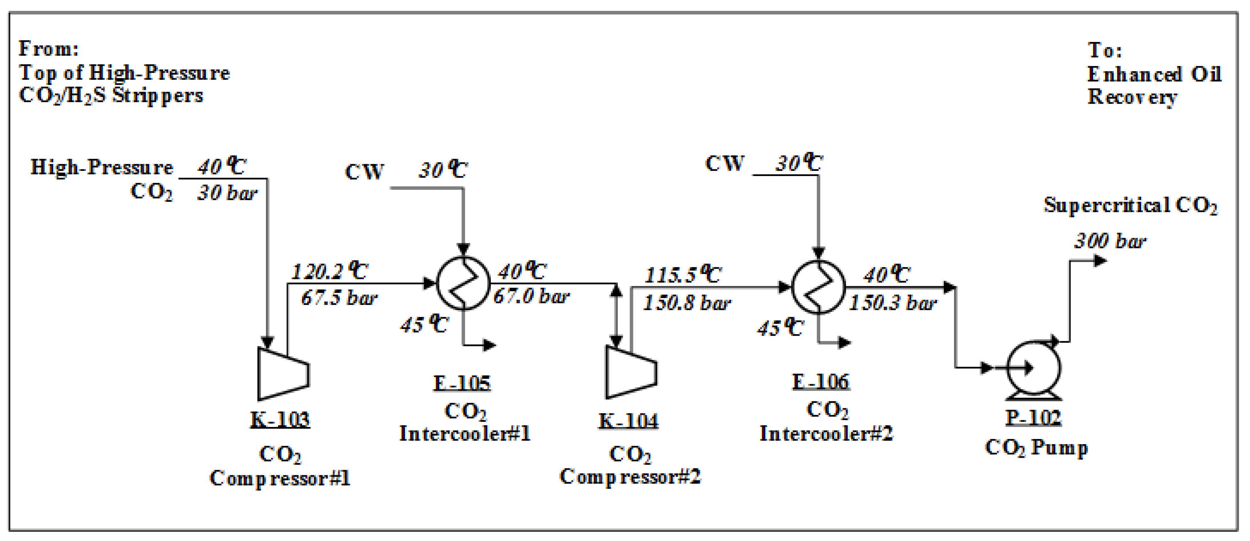
| Compressors | Adiabatic-Efficiency = 75%; Compression-RatioStage = 3 (Landfill-Gas); Compression-RatioStage = 2.25 (CO2-to-EOR). |
| Pumps | Adiabatic-Efficiency = 75%. |
| Intercoolers | TGas-Out = 40 °C; ΔPGas = 0.5 bar. |
| Exchangers | . |
| Cooling-Water | . |
| Chilled-Water | . |
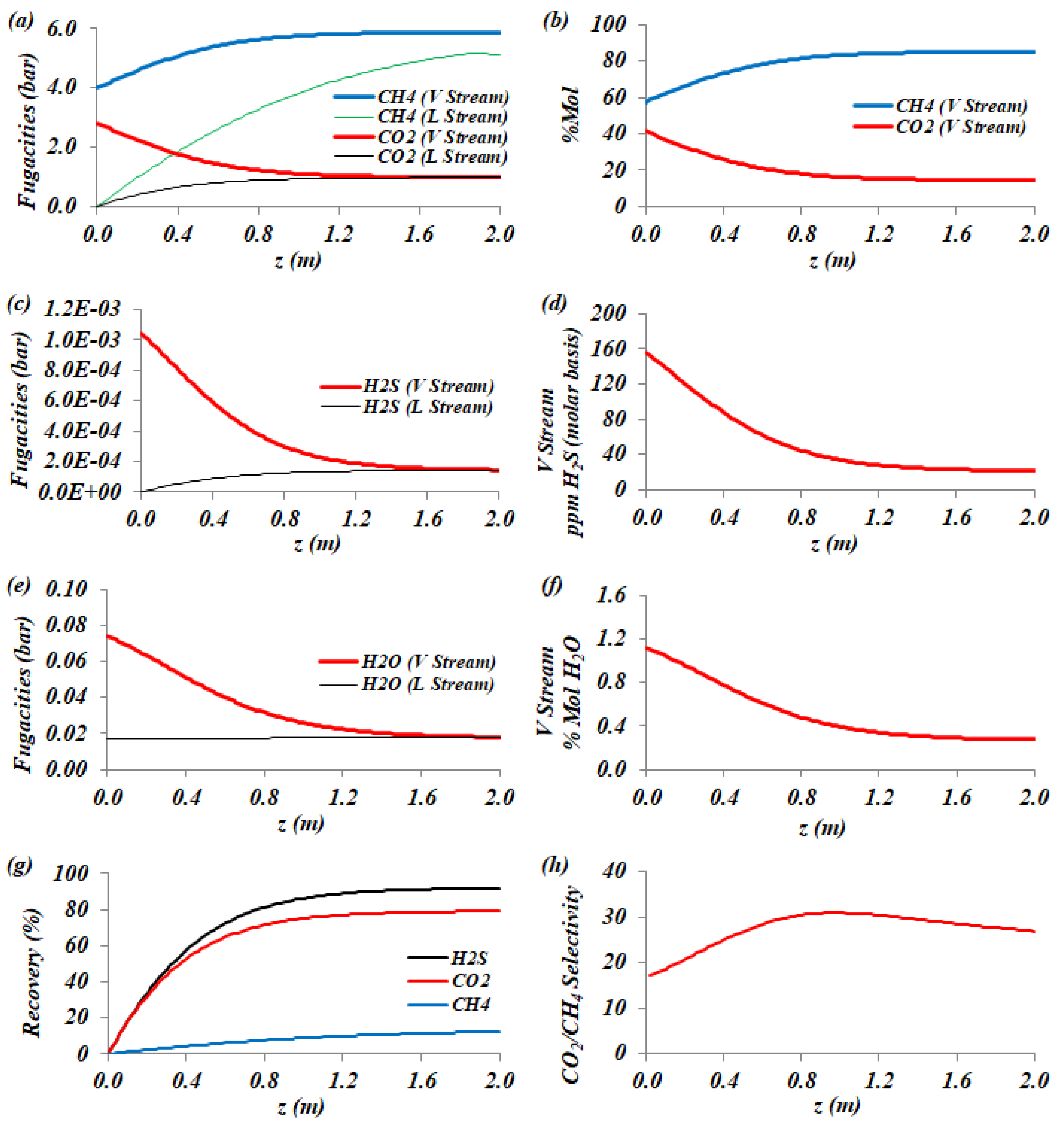
| Streams | Fugacity | CO2 | CH4 | H2S | H2O |
|---|---|---|---|---|---|
| Inlets | (bar) | 2.812 | 3.989 | 0.074 | |
| (bar) | 0 | 0 | 0.017 | ||
| GLMC-CCC-D Outlets | (bar) | 0.203 | 6.669 | 0.019 | |
| (bar) | 1.190 | 3.899 | 0.018 | ||
| GLMC-PC-D Outlets | (bar) | 0.989 | 5.876 | 0.018 | |
| (bar) | 0.977 | 5.120 | 0.017 |
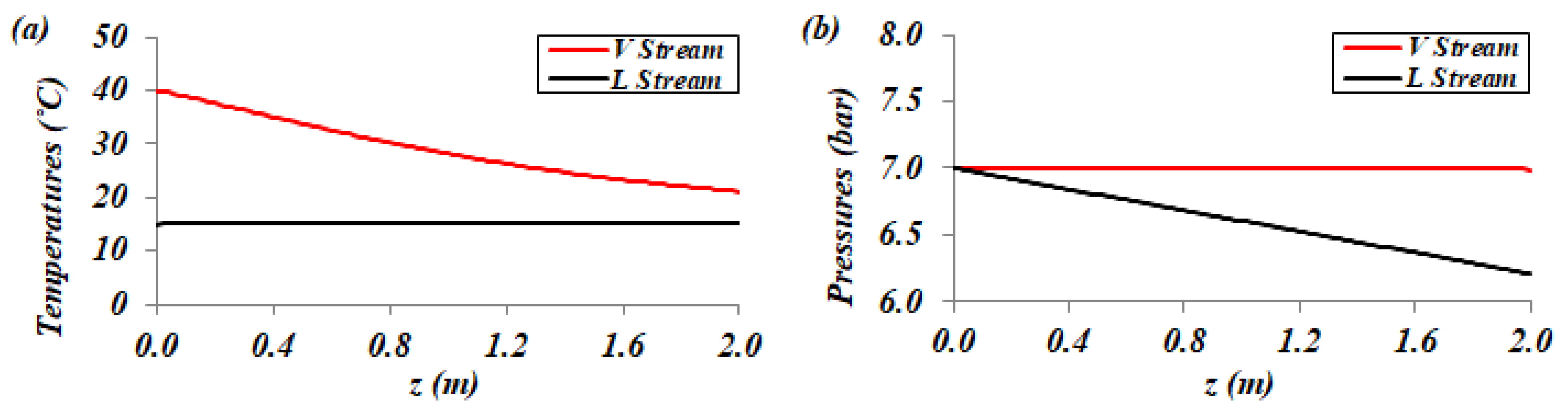
| Landfill-Gas Inlet | Water Inlet | GLMC-CCC-D Landfill-Gas Outlet | GLMC-CCC-D Water Outlet | GLMC-PC-D Landfill-Gas Outlet | GLMC-PC-D Water Outlet | |
|---|---|---|---|---|---|---|
| P (bar) | 7.0 | 7.0 | 6.995 | 6.213 | 6.996 | 6.211 |
| T (°C) | 40.00 | 15.00 | 17.29 | 15.37 | 21.11 | 15.32 |
| MMNm3/d | 0.483961 | - | 0.261854 | - | 0.286783 | - |
| kg/h | - | 7,259,307 | - | 7,275,950 | - | 7,273,439 |
| H2O (%mol) | 1.11 * | 100 | 0.29 | 99.90 | 0.28 | 99.91 |
| CH4 (%mol) | 57.55 | 96.71 | 0.01 | 85.14 | 0.02 | |
| CO2 (%mol) | 41.32 | 3.0 | 0.09 | 14.59 | 0.07 | |
| H2S (ppm-mol) | 154.94 | 4.94 | 0.34 | 21.53 | 0.32 | |
| D3 (ppb-mol) # | 50.97 | 0 | 94.21 | 0 | 86.02 | 0 |
| D4 (ppb-mol) # | 977.59 | 0 | 1806.79 | 0 | 1649.73 | 0 |
| D5 (ppb-mol) # | 1.16 | 0 | 2.15 | 0 | 1.96 | 0 |
| D6 (ppb-mol) # | 12.46 | 0 | 23.03 | 0 | 21.03 | 0 |
| L2 (ppb-mol) # | 865.09 | 0 | 1598.87 | 0 | 1459.89 | 0 |
| L4 (ppb-mol) # | 2.84 | 0 | 5.24 | 0 | 4.79 | 0 |
| L6 (ppb-mol) # | 0.50 | 0 | 0.93 | 0 | 0.85 | 0 |
| Siloxanes (ppb-mol) # | 1910.61 | 0 | 3531.22 | 0 | 3224.27 | 0 |
| Final Results: Gas-to-Solvent CO2/H2S %Recoveries and Gas-to-Solvent CH4 %Loss | ||||||
| GLMC Battery | %Recovery CO2 | %Recovery H2S | %Loss CH4 | |||
| GLMC-PC-D | 79.08 | 91.77 | 12.33 | |||
| GLMC-CCC-D | 96.08 | 98.28 | 9.07 | |||
| Inlet Landfill-Gas | Outlet Landfill-Gas | Stripper Top Gas | Excess Water | |
|---|---|---|---|---|
| H2O (kmol/h) | 10.03 | 1.43 | 1.28 | 7.32 |
| CH4 (kmol/h) | 518.05 | 471.05 | 47.00 | |
| CO2 (kmol/h) | 372.00 | 14.59 | 357.41 | |
| H2S (kmol/h) | 0.1395 | 0.0024 | 0.1371 | |
| High-Pressure CO2/H2S Stripper—Water Regeneration | ||||
| Stripper Top Gas | Lean Water | |||
| P (bar) | 30.0 | 30.2 | ||
| T (°C) | 40.0 | 233.8 | ||
| kmol/h | 405.82 | 402,960.11 | ||
| MMNm3/d | 0.218 | - | ||
| H2O (%mol) | 0.31 | 100 | ||
| CH4 (%mol) | 11.58 | |||
| CO2 (%mol) | 88.07 | |||
| H2S (ppm-mol) | 337.78 | |||
| Biomethane Outlet | Absorber Rich DEPG | Stripper Top Gas | Lean DEPG | |
|---|---|---|---|---|
| P (bar) | 6.9 | 6.995 | 1.1 | 1.2 |
| T (°C) | 15.84 | 19.35 | 88.72 | 175 |
| kmol/h | 485.28 (0.26 MMNm3/d) | 36.86 | 1.80 | 35.06 |
| DEPG (%mol) | 75.98 | 79.87 | ||
| H2O (%mol) | 0.31 | 22.12 | 61.09 | 20.13 |
| CH4 (%mol) | 96.97 | 1.24 | 25.54 | |
| CO2 (%mol) | 2.96 | 0.65 | 13.26 | |
| H2S (ppm-mol) | 4.36 (6.7 mg/Nm3) | 7.77 | 159.44 | |
| D3 (ppm-mol) | 1.25 | 25.6 | ||
| D4 (ppm-mol) | 23.9 | 490 | ||
| D5 (ppm-mol) | 0.00145 | 12.2 | 12.8 | |
| D6 (ppm-mol) | 0.00025 | 57.2 | 5.09 | 59.9 |
| L2 (ppm-mol) | 21.1 | 434 | ||
| L4 (ppm-mol) | 0.00001 | 0.1935 | 1.59 | 0.122 |
| L6 (ppm-mol) | 0.0123 | 0.253 | ||
| Siloxanes (ppm-mol) | 0.0017 (0.029 mg/Nm3) | 116 | 957 | 72.8 |
| Inlet Landfill-Gas | Outlet Biomethane | Top-Gas Stripper | DEPG Make-Up | |
|---|---|---|---|---|
| DEPG (kmol/h) | 0 | |||
| H2O (kmol/h) | 1.43 | 0.33 | 1.10 | 0 |
| CH4 (kmol/h) | 471.05 | 470.59 | 0.46 | - |
| CO2 (kmol/h) | 14.59 | 14.35 | 0.24 | - |
| H2S (kmol/h) | 0.0024 | 0.0021 | 0.0003 | - |
| Siloxanes (kmol/h) | - | |||
| Process Wastes | Power and Utilities Consumption | |||
| Residual Gas | Residual Water | Consumption | ||
| kmol/h | 0.76 | 1.04 | Power | 9.41 MW |
| DEPG (%mol) | 0 | 0 | Chilled Water | 16,461 t/h |
| H2O (%mol) | 7.44 | 99.99 | Cooling Water | 225,507 t/h |
| CH4 (%mol) | 60.77 | 0.00124 | LPS | 4 t/h |
| CO2 (%mol) | 31.53 | 0.01 | MPS | 8604 t/h |
| H2S (ppm-mol) | 378.76 | 0.45 | ||
| Siloxanes (ppm-mol) | 2200 | 7.71 | ||
Disclaimer/Publisher’s Note: The statements, opinions and data contained in all publications are solely those of the individual author(s) and contributor(s) and not of MDPI and/or the editor(s). MDPI and/or the editor(s) disclaim responsibility for any injury to people or property resulting from any ideas, methods, instructions or products referred to in the content. |
© 2024 by the authors. Licensee MDPI, Basel, Switzerland. This article is an open access article distributed under the terms and conditions of the Creative Commons Attribution (CC BY) license (https://creativecommons.org/licenses/by/4.0/).
Share and Cite
da Cunha, G.P.; de Medeiros, J.L.; Araújo, O.d.Q.F. Novel Landfill-Gas-to-Biomethane Route Using a Gas–Liquid Membrane Contactor for Decarbonation/Desulfurization and Selexol Absorption for Siloxane Removal. Processes 2024, 12, 1667. https://doi.org/10.3390/pr12081667
da Cunha GP, de Medeiros JL, Araújo OdQF. Novel Landfill-Gas-to-Biomethane Route Using a Gas–Liquid Membrane Contactor for Decarbonation/Desulfurization and Selexol Absorption for Siloxane Removal. Processes. 2024; 12(8):1667. https://doi.org/10.3390/pr12081667
Chicago/Turabian Styleda Cunha, Guilherme Pereira, José Luiz de Medeiros, and Ofélia de Queiroz F. Araújo. 2024. "Novel Landfill-Gas-to-Biomethane Route Using a Gas–Liquid Membrane Contactor for Decarbonation/Desulfurization and Selexol Absorption for Siloxane Removal" Processes 12, no. 8: 1667. https://doi.org/10.3390/pr12081667