Response Surface Methodology Applied to Cyanobacterial EPS Production: Steps and Statistical Validations

Abstract

Understanding the impact of variables involved in soluble-extracellular polymeric substance (S-EPS) production processes is crucial for reducing production costs and enhancing sustainability. Response surface methodology (RSM) provides essential tools that assist in developing predicted interactions among process variables for both industrial and non-industrial applications. The present study offers a simple and systematic demonstration of RSM capabilities, focusing on maximizing efficiency and minimizing production costs of S-EPS produced by Cyanocohniella rudolphia. RSM was employed to (1) design the production setup; (2) fit the collected data into a second-order polynomial model; (3) statistically evaluate the model’s validity and the significance of the involved variables; and (4) identify and optimize production variables to enhance output and reduce costs. Focused on four key variables, each at three levels, RSM designed 25 distinct S-EPS production conditions, each with three replicates. Statistical analysis identified the most significant variables affecting S-EPS production as the culture medium/wet biomass ratio, production days, and nitrogen concentration. The model’s validation demonstrated a strong correlation between the predicted and experimental values, with S-EPS production ranging from 70.46 to 228.65 mg/L and a maximum variation of 11.6%. This study demonstrates the effectiveness of RSM in optimizing S-EPS production, with the developed model showing a strong correlation between the variables and the response. The RSM model offers a promising approach for the bioprocessing industry, enhancing productivity and efficiency, minimizing costs, and leading to sustainable, cost-effective practices.

1. Introduction

Extracellular polymeric substances (EPSs) are high-molecular-weight compounds, predominantly composed of polysaccharides, which can be secreted by microalgae and cyanobacteria into their surrounding environment. Soluble EPSs (S-EPSs) are a specific subset of these substances that remain dissolved in the culture medium and are usually discarded. However, based on their characteristics and potential applications in various fields, these S-EPS deserve the attention of the scientific community.

To fully realize the potential of cyanobacteria-based S-EPS production and maximize its industrial value, it is crucial to enhance S-EPS production and improve its subsequent utilization. Optimizing the production conditions for S-EPS by cyanobacteria is essential for achieving higher yields. Various physicochemical parameters, such as light intensity and photoperiod, nutrient availability and sources, temperature, and pH, significantly impact S-EPS production in cyanobacteria [1,2].

A systematic approach, such as response surface methodology (RSM) [3,4,5], is needed to identify the key factors and their optimal levels to maximize S-EPS synthesis by cyanobacteria. RSM can employ designs such as Central Composite Design (CCD), Box-Behnken, or Doehlert designs. The choice between these designs should be based on the specific nature of the problem, practical limitations, and study objectives. CCD has advantages over the others, being applied to a wide variety of RSM studies. Box-Behnken is advantageous when aiming to minimize the number of experiments and avoid extreme points in the experimental space. Doehlert is useful for studies requiring uniform coverage of the experimental space with flexibility in the number of factors and levels [6]. RSM utilizes advanced statistical techniques to develop models that predict interactions among process variables and demonstrate how these variables influence the response. This methodology provides essential tools for both industrial and non-industrial processes. The different steps involved in RSM (Figure 1) are as follows:

• Step 1—Experimental design—creation of fractional factorial production design;
• Step 2—Polynomial model—fitting of collected data into a second-order polynomial model;
• Step 3—Model validation—a statistical evaluation of the model’s validity and the assessment of the significance of the involved independent variables;
• Step 4—Response optimization—identification of optimal independent variables to secure the best possible outcomes.

While the one-factor-at-a-time method can effectively test the independent variables, it overlooks potential interactions between them. Therefore, a three-level (low, medium, and high) fractional factorial experimental design should be employed to evaluate how different parameters (variables and levels) influence the response (Step 1).

When using CCD, the number of experimental conditions (N) is determined using Equation (1) and depends on the number of independent variables (k) and n_c, the number of center points.

$$N=2^k+2k+n_c.$$

(1)

In a CCD, the design typically includes the following: (1) factorial points, which are combinations of the lowest and highest levels of the independent variables; (2) star points, located at a distance α from the center values; and (3) center points, repeated multiple times at the central values of all independent variables to estimate experimental error and improve model reliability. Thus, for a given k and a specified n_c, a total number of experiments was defined. This structured approach ensures a robust design that allows for a comprehensive analysis of the independent variables and their interactions.

The collected experimental data can be analyzed to formulate the second-order polynomial model (Step 2), achieved using a quadratic polynomial regression equation (Equation (2)). This equation consists of the response Y, the independent variables $X_i$ and $X_j$, the model constant ${\beta }_0$, the first-order model coefficients ${\beta }_i$ for each independent variables, the quadratic coefficients ${\beta }_{ii}$ for each independent variable $i$, the interaction coefficient ${\beta }_{ij}$ for the interaction between variables $i$ and $j$, and ε, the error term that represents the variability not explained by the model [3].

$$Y={\beta }_0+\Sigma {\beta }_i{X}_i+\Sigma {\beta }_{ij }{X}_i{X}_j+\Sigma {\beta }_{ii}{X}_i^2+\epsilon$$

(2)

Model validation involves several statistical analyses (Step 3); these included assessing residuals to estimate model adequacy, evaluating the lack of fit between the predicted and experimental responses, and analyzing F-values and p-values from ANOVA tests. Statistical analysis can also be useful in studying the influence of each independent variable and simplifying the model for easier practical application.

Additionally, RSM can be applied to determine the optimal independent variables to secure the best response, whether by minimizing or maximizing these variables according to the pretended goal (Step 4). In terms of practical applicability, optimizing these variables aims to enhance output and reduce costs.

Based on this, and to demonstrate in a simple way the most relevant key points of RSM, the study used the production of S-EPS by Cyanocohniella rudolphia as a case study. By employing RSM, the production setup was designed, a polynomial model was developed and validated, and key variables were optimized to make the process more efficient and economical.

2. Experimental Design

2.1. S-EPS Production and Determination

Cyanocohniella rudolphia (BEA 0786B) was provided by the Collection at the Spanish Bank of Algae. The cyanobacteria were cultured in a continuously aerated Spirulina medium with an initial pH of 9.0. The conditions set were an irradiance of 40 μmol photons/m²/s, a 14/10 h light/dark cycle, and a temperature of 22 ± 1 °C. To study the variation in phosphorus and nitrogen concentrations in the RSM application, the concentrations of phosphorus (as K₂HPO₄) and nitrogen (as NaNO₃) were adjusted in the Spirulina medium. The S-EPS production was assessed using the Alcian Blue method. To ensure precise quantification, a calibration curve was constructed with purified S-EPS derived from an axenic culture of C. rudolphia, following the procedures described by Rodrigues et al. [7].

2.2. RSM Methodology

RSM was employed to develop mathematical models with experimental data from C. rudolphia S-EPS production through the CCD methodology (Figure 1). The optimization algorithm utilized was the least squares method, implemented via the Design-Expert software (version 13). This algorithm fits the collected data into a second-order polynomial model by minimizing the sum of the squares of the differences between the observed and predicted values, ensuring the best fit for the experimental data. A three-level factorial design and a four-variable fractional factorial experimental design were performed during the experiment (

Table 1. Independent variables and respective experimental levels used for the optimization of C. rudolphia-based S-EPS production.

Independent Variables	Units	Type of Variable	Variable Level *
			−1	0	+1
Ratio (culture medium/wet biomass) (R)	mL/g	Continuous	1:1	7.5:1	14:1
Days (D)	days	Discrete	1	4	7
Nitrogen concentration (N)	g/L	Continuous	2.50	6.25	10.00
Phosphorus concentration (P) #	g/L	Continuous	0.50	1.25	2.00

* α = 1 was used. ^# the simplified model with three levels and three variables was used, maintaining the phosphorus concentration at 0.50 g/L.

). For the simplified model, after the statistical analysis (Step 3; Figure 1) of the significance of the variables, an optimization algorithm with three levels and three variables (ratio, days, and nitrogen concentration) was conducted, maintaining the phosphorus concentration at 0.50 g/L and using the same significant variable levels as in the general model (Table 1). A face-centered CCD (α = 1) was used to ensure that the star points were equally distanced from the center. As the goal was to maximize S-EPS production, a value of 1 was assigned to the Desirability function.

The selected independent variables and their level ranges were as follows: culture medium/wet biomass ratio (R) (ranging from 1:1 to 14:1 (v/w)), number of production days (ranging from 1 to 7 days), phosphorus concentration (phosphate from K₂HPO₄) (ranging from 0.5 to 2 g/L), and nitrogen concentration (nitrate from NaNO₃) (ranging from 2.5 to 10 g/L). The specific value of α (α = 1) was determined to ensure that the star points were equally distanced from the center. Using Equation (1) for the four independent variables (k = 4) and their respective levels (n_c = 9), 25 different S-EPS production conditions (N) were generated (

Table 2. RSM experimental design with three levels and four variables for C. rudolphia-based S-EPS experimental response and model-predicted response obtained by the general model (Equation (4)).

N	Independent Variables—Production Conditions (Coded Levels) ^				Response—S-EPS Production (mg/L) #
	Ratio (Culture Medium/Wet Biomass) (mL/g)	Production Days (D; day)	Phosphorus Concentration (P; g/L)	Nitrogen Concentration (N; g/L)	Experimental Values	Predicted Values	Variation (%) *
1	1:1 (−1)	1 (−1)	0.50 (−1)	2.50 (−1)	192.86 ± 8.55	199.52	−3.45
2	1:1 (−1)	1 (−1)	0.50 (−1)	10.00 (+1)	217.92 ± 12.28	208.79	4.19
3	1:1 (−1)	1 (−1)	2.00 (+1)	2.50 (−1)	224.53 ± 5.66	225.52	−0.44
4	1:1 (−1)	1 (−1)	2.00 (+1)	10.00 (+1)	228.65 ± 16.31	228.97	−0.14
5	1:1 (−1)	7 (+1)	0.50 (−1)	2.50 (−1)	199.64 ± 63.96	186.90	6.38
6	1:1 (−1)	7 (+1)	0.50 (−1)	10.00 (+1)	178.69 ± 21.11	194.32	−8.75
7	1:1 (−1)	7 (+1)	2.00 (+1)	2.50 (−1)	200.96 ± 14.04	203.96	−1.49
8	1:1 (−1)	7 (+1)	2.00 (+1)	10.00 (+1)	206.82 ± 2.94	203.73	1.49
9	14:1 (+1)	1 (−1)	0.50 (−1)	2.50 (−1)	70.46 ± 8.82	67.56	4.12
10	14:1 (+1)	1 (−1)	0.50 (−1)	10.00 (+1)	112.49 ± 0.77	113.89	−1.24
11	14:1 (+1)	1 (−1)	2.00 (+1)	2.50 (−1)	72.73 ± 8.52	61.51	15.43
12	14:1 (+1)	1 (−1)	2.00 (+1)	10.00 (+1)	93.44 ± 3.37	100.19	−7.22
13	14:1 (+1)	7 (+1)	0.50 (−1)	2.50 (−1)	143.40 ± 8.69	149.33	−4.14
14	14:1 (+1)	7 (+1)	0.50 (−1)	10.00 (+1)	200.78 ± 11.09	193.80	3.48
15	14:1 (+1)	7 (+1)	2.00 (+1)	2.50 (−1)	131.20 ± 5.19	134.34	−2.39
16	14:1 (+1)	7 (+1)	2.00 (+1)	10.00 (+1)	173.40 ± 14.18	171.16	1.29
17	7.5:1 (0)	4 (0)	1.25 (0)	6.25 (0)	160.31 ± 15.66	142.34	11.21
18	1:1 (−1)	4 (0)	1.25 (0)	6.25 (0)	226.75 ± 1.55	205.61	9.32
19	7.5:1 (0)	1 (−1)	1.25 (0)	6.25 (0)	115.44 ± 10.65	128.88	−11.64
20	7.5:1 (0)	4 (0)	0.50 (−1)	6.25 (0)	132.21 ± 1.17	143.34	−8.42
21	7.5:1 (0)	4 (0)	1.25 (0)	2.50 (−1)	120.24 ± 8.22	129.03	−7.31
22	7.5:1 (0)	4 (0)	2.00 (+1)	6.25 (0)	130.89 ± 4.07	142.34	−8.75
23	7.5:1 (0)	4 (0)	1.25 (0)	10.00 (+1)	157.07 ± 2.98	155.65	0.90
25	7.5:1 (0)	7 (+1)	1.25 (0)	6.25 (0)	162.24 ± 5.61	155.80	3.97
25	14:1 (+1)	4 (0)	1.25 (0)	6.25 (0)	135.24 ± 6.75	125.91	6.90

N: number of experimental conditions determined using CCD (Equation (1)). * Variation (%) = [(experimental value − predicted value)/experimental value) × 100)]. ^# mean ± standard deviation of the replicates: 3 replicates for the factorial and star points and 6 replicates for the center point (total of 78 trials). ^ Variable-coded levels: low (−1); medium (0); high (+1).

) and performed experimentally in triplicate (step 1). The CCD included 16 factorial points (N 1 to 16), 8 star points (N 18 to 25), and 1 repeated center point (N 17, repeated 6 times). The arrangement of the input variables is detailed in Table 2.

Considering these independent variables (R, D, P, and N) and their respective levels (Table 1) employed in this experimental design, a quadratic equation was specifically derived (Equation (3)) to correlate with the experimental responses obtained (Step 2).

$$\begin{array}{l}Y={ X}_0+{ X}_{1}R+{ X}_{2}D+X_{3}P+{ X}_{4}N+{ X}_{12}R*D+X_{13}R*P+{ X}_{14}R*N+\\ { X}_{23}D*P+{ X}_{24}D*N+{ X}_{34}P*N+{ X}_{11}R*R+{ X}_{22}D*D+{ X}_{33}P*P+{ X}_{44}N*N+\epsilon \end{array}$$

(3)

3. Results and Discussion

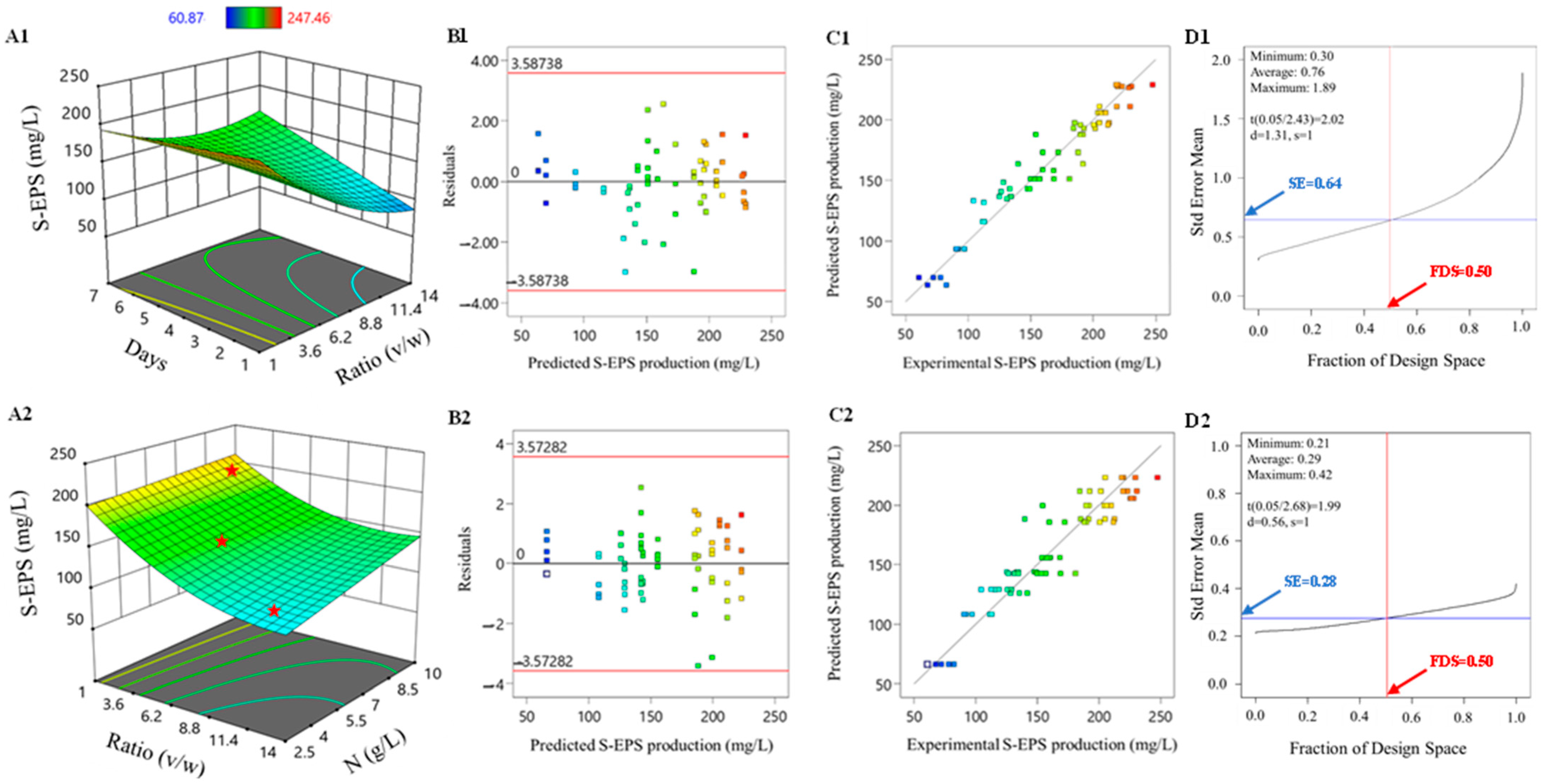
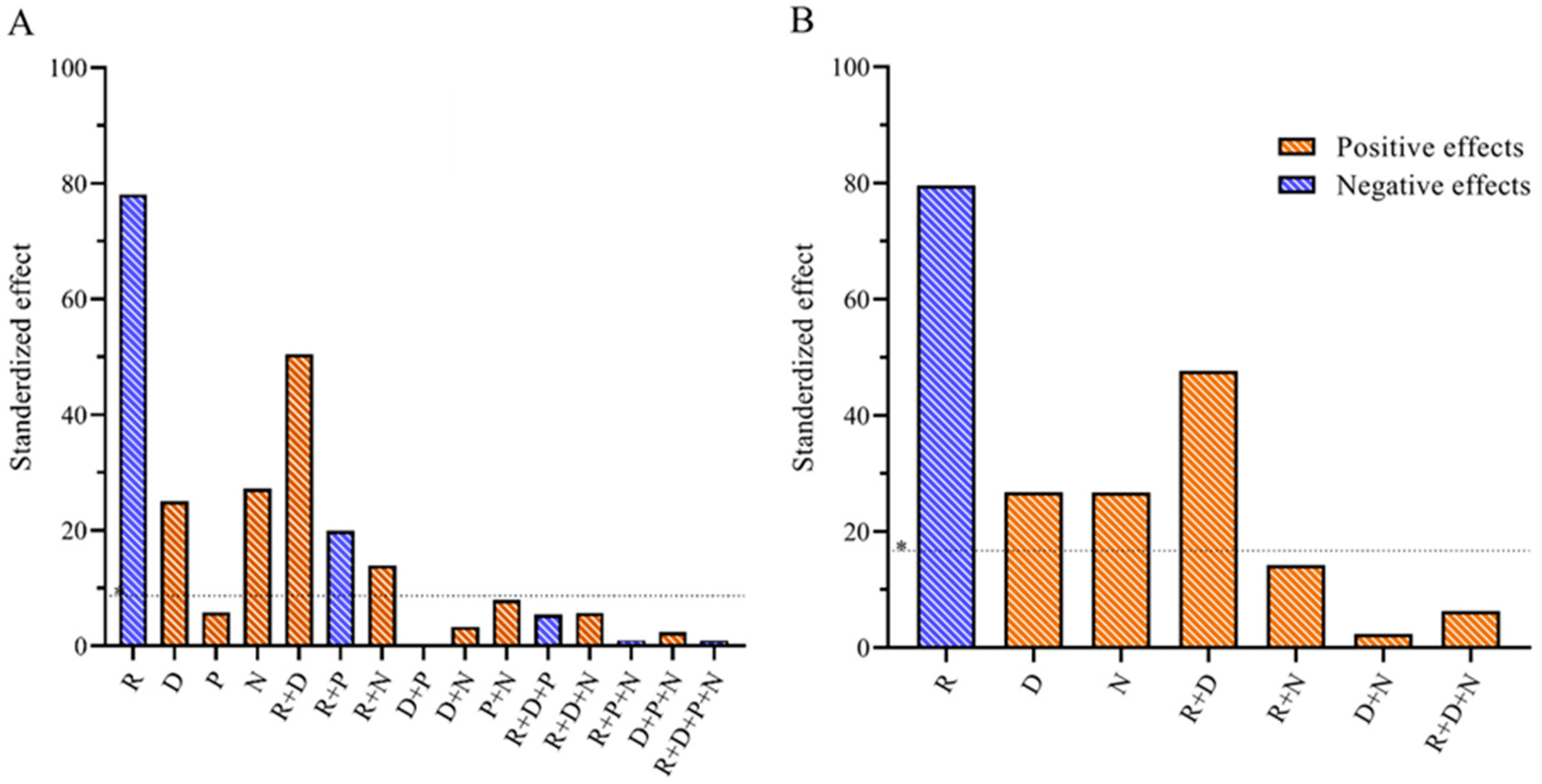
3.1. RSM Model: Application, Refinement, and Validation Applications to Response Optimization

Based on the experimental design set-up and the corresponding results obtained for S-EPS production (summarized in Table 2), a second-order polynomial model was obtained as follows:

$$\begin{array}{r}\mathrm{S}-\mathrm{EPS} \mathrm{production} (\mathrm{mg}/\mathrm{L})=147.43-41.31R+14.92D+0.788P+11.8N+23.6R*D-8.01R*P\\ +9.26R*N-2.23D*P-0.4639D*N -1.91P*N+37.87R*R-4.29D*D-11.57P*P-4.47N*N\end{array}$$

(4)

This model (referred to as the general model) elucidates the relationship between the independent variables (production conditions) and the response (C. rudolphia-based S-EPS production). The model enables the prediction or estimation of C. rudolphia-based S-EPS production under various experimental conditions, which can be visualized in 3D models (Figure 2A1).

In these specific experimental setups, the cyanobacteria produced S-EPS ranging from 70.46 to 228.65 mg/L. This range aligns with the RSM model’s estimated S-EPS production, which ranges from 67.56 to 228.97 mg/L (Table 2). The maximum percentage variation between the experimental and predicted values was 11.64%. To further assess the precision of the model across the entire design space, the Fraction of Design Space (FDS) analysis was performed. The FDS plot (Figure 2D1) illustrates the prediction variance across the design space, confirming the precision and reliability of the model and demonstrating its effectiveness in estimating S-EPS production.

The statistical analysis, which includes the evaluation of residuals (Figure 2B1), lack-of-fit, and ANOVA (

Table 3. Analysis of variance (ANOVA) applied to the general model (Equation (4)).

	Sum of Squares	Degree of Freedom	Mean Square	F-Value	p-Value
Model	1.59 × 105	14	11,361.83	40.06	<0.0001
R	92,171.23	1	92,171.23	325.02	<0.0001
D	12,026.63	1	12,026.63	42.41	<0.0001
P	33.53	1	33.53	0.12	0.7321
N	7578.77	1	7578.77	26.72	<0.0001
R*D	26,725.88	1	26,725.88	94.24	<0.0001
R*P	3082.14	1	3082.14	10.87	0.0016
R*N	4119.63	1	4119.63	14.53	0.0003
D*P	239.76	1	239.76	0.85	0.3614
D*N	10.33	1	10.33	0.04	0.8492
P*N	175.79	1	175.79	0.62	0.4340
R*R	11,017.20	1	11,017.20	38.85	<0.0001
D*D	141.23	1	141.23	0.50	0.4830
P*P	1029.33	1	1029.33	3.63	0.0613
N*N	153.57	1	153.57	0.54	0.4645
Residual	17,865.95	63	283.59	-----	-----
Lack of Fit	4834.92	10	483.49	1.97	0.0561
Error	13,031.03	53	245.87	-----	-----

* R: culture medium/wet biomass ratio; D: production days; P: phosphorus concentration; N: nitrogen concentration.

), confirms the model’s applicability. The scatterplot of residual vs. predicted values showed a uniform distribution, indicating normality (R² = 0.9417) and the absence of outliers (Figure 2C1).

For practical applications, simplifying the model is often crucial, especially when dealing with a large number of independent variables. This simplification can be achieved by analyzing the significance of each variable, as exemplified in Figure 3A, where ANOVA analysis provided insights into the significance of the model’s independent variables. The p-value and F-value (Table 3) indicated that the R, D, and N variables were significant, whereas variations in P (phosphorus concentration) did not significantly affect the response. Since the P variable was not significant, the experimental design was refined (optimized algorithm) to focus on the three significant independent variables (R, D, and N), reducing the number of experimental conditions to 15 (

Table 4. RSM fractional experimental design with three levels and three variables for C. rudolphia-based S-EPS experimental production and model-predicted response obtained by the simplified model (Equation (5)). Phosphorus concentration: 0.50 g/L.

N	Independent Variables—Production Conditions (Coded Levels) ^			Response—S-EPS Production (mg/L) #
	Ratio (Culture Medium/Wet Biomass) (mL/g)	Production Days (D; day)	Nitrogen Concentration (N; g/L)	Experimental Values	Predicted Values	Variation (%) *
1	1:1 (−1)	1 (−1)	2.50 (−1)	211.70 ± 9.41	212.47	−0.36
2	1:1 (−1)	1 (−1)	10.00 (+1)	219.65 ± 1.19	218.56	0.50
3	1:1 (−1)	4 (0)	6.25 (0)	200.49 ± 8.49	222.09	−10.77
4	1:1 (−1)	7 (+1)	2.50 (−1)	197.60 ± 8.49	196.05	0.78
5	1:1 (−1)	7 (+1)	10.00 (+1)	205.42 ± 7.06	200.29	2.50
6	7.5:1 (0)	1 (−1)	6.25 (0)	142.06 ± 1.79	123.70	12.92
7	7.5:1 (0)	4 (0)	2.50 (−1)	128.03 ± 1.20	126.58	1.13
8	7.5:1 (0)	4 (0)	6.25 (0)	149.15 ± 14.00	146.15	2.01
9	7.5:1 (0)	4 (0)	10.00 (+1)	154.73 ± 3.56	150.28	2.88
10	7.5:1 (0)	7 (+1)	6.25 (0)	155.86 ± 2.50	153.54	1.49
11	14:1 (+1)	1 (−1)	2.50 (−1)	65.57 ± 4.44	64.12	2.21
12	14:1 (+1)	7 (+1)	2.50 (−1)	138.18 ± 1.54	142.08	−2.82
13	14:1 (+1)	1 (−1)	10.00 (+1)	104.80 ± 8.88	107.27	−2.36
14	14:1 (+1)	7 (+1)	10.00 (+1)	183.01 ± 5.10	183.38	−0.20
15	14:1 (+1)	4 (0)	6.25 (0)	136.31 ± 4.76	139.46	−2.31

N: number of experimental conditions determined using the CCD (Equation (1)). * Variation (%) = [(experimental value − predicted value)/experimental value) × 100)]. ^# mean ± standard deviation of the replicates: 3 replicates for the factorial and star points, and 6 replicates for the center point (total of 48 trials). ^ Variable-coded levels: low (−1); medium (0); high (+1).

). These conditions included eight factorial points, six star points, and one center point (Equation (1); N = 2³ + 2 × 3 + 1 = 15; center point repeated six times). Each condition was performed in triplicate, resulting in a total of 48 trials instead of the previous 78. With this experimental simplification, the previously identified mathematical model (general model, Equation (4)) was streamlined into a more simplified model (Equation (5)).

$$\mathrm{S}-\mathrm{EPS} \mathrm{production} (\mathrm{mg}/\mathrm{L})=142.34–39.85R+13.46D+13.31N+25.24R*D+7.62R*N+23.41R*R$$

(5)

The simplified model (Equation (5)) demonstrated improved prediction accuracy compared to the general model (Equation (4)), as evidenced by the lower F-value for the residual lack-of-fit (

Table 5. Analysis of variance (ANOVA) applied to the simplified model (Equation (5)).

	Sum of Squares	Degree of Freedom	Mean Square	F-Value	p-Value
Model	1.467 × 105	6	24,450.32	92.48	<0.0001
R	83,999.52	1	83,999.52	317.72	<0.0001
D	9583.41	1	9583.41	36.25	<0.0001
N	9370.07	1	9370.07	35.44	<0.0001
R*D	29,880.44	1	29,880.44	113.02	<0.0001
R*N	2721.69	1	2721.69	10.29	0.0020
R*R	9050.72	1	9050.72	34.23	<0.0001
Residual	18,506.94	70	264.38
Lack of Fit	3586.34	8	448.29	1.86	0.0823
Error	14,920.61	62	240.65

* $R$: culture medium/wet biomass ratio; D: production days; N: nitrogen concentration.

). The reduction in the F-value from the general model’s 1.97 to 1.86 in the simplified model suggests an enhanced fit to the data, signifying an improvement in predictive performance. Despite a slight decrease in the R² value to 0.8880 (

Table 6. Comparative statistical analysis of responses using the general (Equation (4)) and simplified models (Equation (5)).

	General Model (Equation (4))	Simplified Model (Equation (5))
Predicted $R^2$	0.9092	0.8629
Adjusted $R^2$	0.9285	0.8784
$R^2$	0.9417	0.8880

), the close alignment between the predicted R² (0.8629) and adjusted R² (0.8784) indicates that the model maintains its robustness. This congruence between the predicted and adjusted R² values suggests that the simplified model, with its refined parameters, offers reliable response predictions, maintaining a high degree of accuracy and applicability.

The analysis of the residuals from the simplified model’s predictions for S-EPS production indicated that they were uniformly distributed (Figure 2C2), consistent with the experimental data (R² = 0.9178), and free from outliers. The uniform distribution demonstrates a strong correlation between the predicted and observed values, indicating the model’s effectiveness in capturing the underlying patterns of the dataset. Through ANOVA statistical analyses, the adequacy of the simplified model’s fit was further validated by a high F-value of 92.48, which significantly exceeds the critical value of F_(0.05,6,70) = 2.215, alongside a p-value smaller than 0.0001 (Table 5). Such statistical evidence robustly supports the simplified model’s ability to accurately represent the relationship between the independent variables and the response, affirming its reliability with a high level of confidence.

Thus, the statistical analysis indicates that the simplified model not only preserves but may also enhance the efficacy of predictive analysis for S-EPS production. Furthermore, this streamlined approach improves clarity, leading to better decision-making and resource management across experimental and industrial environments.

Regarding S-EPS production, the simplified model predicts that S-EPS production ranges from 64.12 to 218.56 mg/L (Figure 2A2; Table 4), aligning closely with both the experimentally obtained S-EPS production (65.57 to 219.65 mg/L) and the range predicted by the general model (67.56 to 228.97 mg/L). The percentage variation between the experimental and predicted responses being less than 10.77% attests to the model’s accuracy in estimating S-EPS production.

The specific value of the Fraction of Design Space (FDS; Figure 2D) and the shape of the FDS curve offer additional insights into the precision and efficiency of the models across different sections of the design space. Using a direct approach to optimize EPS production (with a Desirability score of 1), an FDS = 0.50 was obtained for both models. However, a significant difference in measurement precision is observed within the 95% confidence interval. This is indicated by the lower standard error of the mean (SE) in the simplified model (SE = 0.28; Figure 2D2) compared to the higher SE in the general model (SE = 0.64; Figure 2D1). This means that 50% of the design space has an SE ≤ 0.28 for the simplified model, while the same 50% for the general model has an SE ≤ 0.64. Regarding the shape of the curve, the flatter curve of the simplified model indicates a more uniformly distributed precision across the entire design space, making it more robust and reliable in predicting C. rudolphia-based S-EPS.

To confirm experimentally the reliability and predictability of the model, combinations of independent variables not included in the experimental design must be used. Ideally, these combinations should span a range of response levels, from the lowest to the highest, as illustrated in Figure 2A2 (points 1–3). Comparing both predicted and experimental responses will experimentally confirm the model’s applicability.

3.2. RSM Model: Applications to Response Optimization

Another significant potential of RSM lies in identifying optimal production variables to achieve the best possible outcomes, a crucial aspect regardless of whether these variables are targeted for minimization or maximization (step 4; Figure 1). Through modeling responses in relation to various production variables, RSM enables the maximization of responses. This capability extends to scenarios without specific conditioning variables as well as to those aimed at reducing production costs, illustrating the versatility and utility of RSM in optimizing production processes to meet effectively diverse industrial and sustainability objectives.

Applying this approach to the study case (Figure 1), for the scenario focused on maximizing S-EPS production (optimum condition) from the cyanobacteria C. rudolphia, the experimental conditions determined by the RSM are 1 g of wet biomass per 1 mL of culture medium for 1 day of production time, 0.98 g/L of phosphorus, and 10 g/L of nitrogen. Under these specific conditions, the achieved S-EPS production by the model would be 223.1 mg/L. Experimentally, for these experimental conditions, a production of 219.08 ± 5.94 mg/L was obtained, which corresponded to a variation of less than 2% between the experimental value and the model-predicted value. Alternatively, in the scenario aimed at minimizing production costs, the R variables proved to be the most significant, with the optimal production conditions being 1 g of wet biomass per 6.87 mL of culture medium for 7 days of production time, 0.98 g/L of phosphorous, and 10 g/L of nitrogen. Under these specific conditions, the achieved S-EPS production would be 113.2 mg/L, obtained when the R variable was intentionally set to its lowest level. Experimentally, for these experimental conditions, a production of 112.75 ± 1.17 mg/L was obtained, which corresponded to a variation of 0.4% between the experimental value and the model-predicted value.

Although the study by Jung et al. [8] on C. rudolphia reported significant tolerance to saline conditions, the production of EPS by C. rudolphia has not yet been quantified, making a direct comparison or evaluation of the results obtained in this study impossible. Nevertheless, compared to published studies on different species and experimental conditions [9,10,11,12,13,14,15,16,17], the values obtained for EPS production by C. rudolphia under optimal conditions are within the range found in these studies for species considered good EPS producers. This indicates that C. rudolphia is a viable species for EPS production. However, the main purpose of this work was to demonstrate that using RSM offers unparalleled advantages over the approach of testing independent variables individually. In contrast, RSM allows for a detailed analysis of the interactions between independent variables, leading to a more precise and efficient optimization of EPS production. Furthermore, RSM requires a significantly lower number of experiments to identify the best experimental conditions, thereby saving time and resources. Additionally, based on the explanation provided in this study, a beginner can easily and intuitively use RSM to create the experimental design, identify the most impactful independent variables on EPS production, model the response, conduct a complete statistical analysis, and identify the best combination of independent variables to ensure the best possible outcomes in terms of production or production costs. Thus, the industrial applicability of RSM for EPS production becomes evident, as the optimized conditions can be easily scaled up for large-scale production. The efficiency and cost reduction achieved through the optimization of production parameters can bring significant economic benefits to the EPS bioprocessing industry.

4. Conclusions

Using the optimization of EPS production by C. rudolphia as a case study, this study explored and demonstrated simply and intuitively the various steps and tools of RSM. This study highlighted the effective application of RSM in optimizing EPS production, using a reduced number of experimental trials compared to traditional methods, thus saving time and resources. The statistical analysis identified the most significant physicochemical parameters affecting EPS production, and the developed polynomial model was applied to optimize the independent variables, aiming for maximum response and cost reduction with a focus on industrial application. The findings underline the potential for scaling up the optimized conditions for industrial applications, promoting sustainable and economical practices in the bioprocessing industry. The approach demonstrated in this study supports enhanced productivity and resource efficiency, paving the way for significant economic benefits in the large-scale production of EPS.

References

1. Cruz, D.; Vasconcelos, V.; Pierre, G.; Michaud, P.; Delattre, C. Exopolysaccharides from cyanobacteria: Strategies for bioprocess development. Appl. Sci. 2020, 10, 3763. [Google Scholar] [CrossRef]
2. Tiwari, O.N.; Khangembam, R.; Shamjetshabam, M.; Sharma, A.S.; Oinam, G.; Brand, J.J. Characterisation and optimisation of bioflocculant exopolysaccharide production by cyanobacteria Nostoc sp. BTA97 and Anabaena sp. BTA990 in culture conditions. Appl. Biochem. Biotechnol. 2015, 176, 1950–1963. [Google Scholar] [CrossRef] [PubMed]
3. Singh, P.; Shera, S.S.; Banik, J.; Banik, R.M. Optimisation of cultural conditions using response surface methodology versus artificial neural network and modelling of L-glutaminase production by Bacillus cereus MTCC 1305. Bioresour. Technol. 2013, 137, 261–269. [Google Scholar] [CrossRef]
4. Reig, S.J.M.; Luti, K.J.K. Response surface methodology: A review on its applications and challenges in microbial cultures. Mater. Today Proc. 2021, 42, 2277–2284. [Google Scholar] [CrossRef]
5. Domagalski, N.R.; Mack, B.C.; Tabora, J.E. Analysis of design of experiments with dynamic responses. Org. Process Res. Dev. 2015, 19, 1667–1682. [Google Scholar] [CrossRef]
6. Meyers, R.H.; Montgomery, D.C.; Anderson-Cook, M.A. Response surface methodology: Process and product optimisation using designed experiments. In Response Surface Methodology; Balding, D.J., Cressie, N.A.C., Fitzmaurice, G.M., Johnstone, I.M., Molenberghs, G., Scott, D.W., Smith, A.F.M., Tsay, R.S., Weisberg, S., Eds.; John Wiley & Sons, Inc.: Hoboken, NJ, USA, 2009. [Google Scholar]
7. Rodrigues, F.; Faria, M.; Gomes, R.; Mendonça, I.; Ferreira, A.; Cordeiro, N. Exopolymers from Cyanocohniella rudolphia: From modelling production to microplastics remediation applications. J. Clean. Prod. 2024, submitted.
8. Jung, P.; Sommer, V.; Karsten, U.; Lakatos, M. Salt tolerance of terrestrial Cyanocohniella strains (Cyanobacteria) and description of C. rudolphia sp. nov. point to a marine origin of the genus and long-distance terrestrial dispersal patterns. Microorganisms 2022, 10, 968. [Google Scholar] [CrossRef]
9. Cunha, C.; Faria, M.; Nogueira, N.; Ferreira, A.; Cordeiro, N. Marine vs freshwater microalgae exopolymers as biosolutions to microplastics pollution. Environ. Pollut. 2019, 249, 372–380. [Google Scholar] [CrossRef] [PubMed]
10. Babiak, W.; Krzemińska, I. Extracellular polymeric substances (EPS) as microalgal bioproducts: A Review of factors affecting eps synthesis and application in flocculation processes. Energies 2021, 14, 4007. [Google Scholar] [CrossRef]
11. Gongi, W.; Pinchetti, J.L.G.; Cordeiro, N.; Sadok, S.; Ouada, H.B. Extracellular polymeric substances produced by the thermophilic cyanobacterium Gloeocapsa gelatinosa: Characterization and assessment of their antioxidant and metal-chelating activities. Mar. Drugs 2022, 20, 227. [Google Scholar] [CrossRef] [PubMed]
12. Reignier, O.; Bormans, M.; Marchand, L.; Sinquin, C.; Amzil, Z.; Zykwinska, A.; Briand, E. Production and composition of extracellular polymeric substances by a unicellular strain and natural colonies of Microcystis: Impact of salinity and nutrient stress. Environ. Microbiol. Rep. 2023, 15, 783–796. [Google Scholar] [CrossRef] [PubMed]
13. Gongi, W.; Cordeiro, N.; Pinchetti, J.L.G.; Sadok, S.; Ben Ouada, H. Extracellular polymeric substances with high radical scavenging ability produced in outdoor cultivation of the thermotolerant chlorophyte Graesiella sp. J. Appl. Phycol. 2021, 33, 357–369. [Google Scholar] [CrossRef]
14. Laroche, C. Exopolysaccharides from microalgae and cyanobacteria: Diversity of strains, production strategies, and applications. Mar. Drugs 2022, 20, 336. [Google Scholar] [CrossRef] [PubMed]
15. Morais, M.G.; Santos, T.D.; Moraes, L.; Vaz, B.S.; Morais, E.G.; Costa, J.A.V. Exopolysaccharides from microalgae: Production in a biorefinery framework and potential applications. Bioresour. Technol. Rep. 2022, 18, 101006. [Google Scholar] [CrossRef]
16. Koçer, A.T.; İnan, B.; Kaptan Usul, S.; Koçer, B.; Çakmak, Y.S.; Usul, M.; Mendi, A.; Gencer, S. Exopolysaccharides from microalgae: Production, characterization, optimization and techno-economic assessment. Braz. J. Microbiol. 2021, 52, 1779–1790. [Google Scholar] [CrossRef] [PubMed]
17. Cunha, C.; Silva, L.; Paulo, J.; Faria, M.; Nogueira, N.; Cordeiro, N. Microalgal-based biopolymer for nano- and microplastic removal: A possible biosolution for wastewater treatment. Environ. Pollut. 2020, 263 Pt B, 114385. [Google Scholar] [CrossRef] [PubMed]
Figure 1. Flowchart illustrating the key steps in the application of RSM for optimizing S-EPS production by C. rudolphia.
Processes 12 01733 g001
Figure 2. 3D Graphical representation (A). Residual plot illustrating the correlation between predicted and experimental responses (B). Comparison between predicted response and experimental response (C) and Fraction of Design Space (FDS) (D) (SE-standard error of the mean; t-tolerance value; 95% confidence interval; d-half-width of the prediction interval; and s-standard deviation of the model’s predictions), obtained by the general (1) and simplified (2) models.
Processes 12 01733 g002
Figure 3. Pareto chart showing the degree of influence of independent variables on S-EPS production by the general model (A) and the simplified model (B). (*) The horizontal line represents the threshold of statistical significance. R: culture medium/wet biomass ratio; D: production cycle time; N: nitrogen concentration; P: phosphorus concentration.
Processes 12 01733 g003