Short-Term Wind Speed Prediction Study Based on Variational Mode Decompositions–Sparrow Search Algorithm–Gated Recurrent Units

Abstract

Improving the accuracy of short-term wind speed predictions is crucial for mitigating the impact on power systems when integrating wind power into an electricity grid. This study developed a hybrid short-term wind speed prediction method, termed VMD–SSA–GRU, by combining variational mode decomposition (VMD) with gated recurrent units (GRUs) and optimizing it using a sparrow search algorithm (SSA). Initially, VMD was used to decompose the wind speed time series into subtime series. After reconstructing these subtime series, a GRU model was employed to establish separate prediction models for each series. Furthermore, an enhanced SSA was proposed to optimize the hyperparameters of the GRU model, which improved the prediction accuracy. Ultimately, the sub-series predictions were aggregated to produce the final wind speed prediction values. The predictive accuracy of this model was validated using the wind speed data measured at a meteorological station near a bridge site. The performance of the VMD–SSA–GRU model was compared with several other hybrid models, including those using wavelet transform, long short-term memory, and other neural networks. Comparably, the RMSE value of the VMD-SSA-GRU model was lower by 25.3%, 60.2%, and 61.7% in comparison to the VMD–SSA–LSTM, VMD–GRU, and VMD–LSTM models, respectively. The experimental results demonstrated that the proposed method achieved higher prediction accuracy than traditional methods.

1. Introduction

Wind power is recognized for its renewability, minimal pollution, and cost-effectiveness, and its contribution to the global energy mix is on the rise [1]. However, the intermittent and variable nature of wind poses challenges for its integration into the electrical grid, which complicates the power system operations. Therefore, the accurate forecasting of wind speed is essential for the effective real-time management of grid-connected power systems. Wind speed forecasting models are primarily categorized into statistical and deep learning models [2,3]. Common statistical approaches include autoregressive models, moving averages, and autoregressive integrated moving average models [4]. Additionally, to address the limitations in accuracy for nonlinear wind speed prediction, deep learning (DL) models have been increasingly adopted. DL is a powerful tool for recognizing the inherent nonlinear attributes of wind speed time series. Categories of short-term wind speed forecasting methods with respect to signal DL models and hybrid DL models are summarized in

Table 1. Categories of Short-term Wind Speed Forecasting Methods.

First Classification	Second Classification	Ref.
Signal model	CNN	[5]
	LSTM	[6]
	BiLSTM	[7]
	GRU	[8]
	TCN	[9]
	Transformer	[10]
Hybrid model	WP-CNN-LSTM	[11]
	WT-DeepAR	[12]
	EEMD-LSTM	[13]
	VMD-CNN-GRU	[14]

.

DL models mainly include convolutional neural networks (CNNs) [5], LSTM networks [6], BiLSTM networks [7], gated recurrent units (GRUs) [8], temporal convolutional networks (TCNs) [9], and transformers [10]. Moreover, hybrid DL models that integrate different algorithms are proposed to further improve the prediction accuracy of wind speeds, which can utilize the unique strengths of disparate forecasting methodologies. For example, Liu et al. [11] employed wavelet packet decomposition on wind speed data and evaluated the performance of various neural networks. Their results indicated that the hybrid model combining CNNs with LSTM yielded the highest prediction accuracy. He et al. [12] introduced a short-term wind speed forecasting method using a deep autoregressive (DeepAR) model and assessed the performance of hybrid models that combined convolutional and recurrent neural networks along with wavelet decomposition for both point and interval forecasting. Yan et al. [13] used a hybrid model of EEMD and LSTM for wind speed prediction in consideration of seasonal features. Zhao et al. [14] proposed a new hybrid deep learning model named VMD-CNN-GRU and demonstrated the effectiveness and competitiveness of the proposed model for forecasting wind power, considering spatio-temporal features. Peng et al. [15] developed a wind power prediction method that integrates the (particle swarm optimization) PSO with the (bidirectional long- and short-term memory) BiLSTM model. By optimizing the hyperparameters of the BiLSTM model through PSO, the prediction accuracy of wind power was significantly improved. Although the hybrid models proposed by researchers have proven effective in predicting wind speeds, they often rely on traditional decomposition algorithms. For instance, wavelet transforms are susceptible to data edge effects, while empirical mode decomposition suffers from low computational efficiency and can lead to mode mixing, which increases prediction errors [16]. Moreover, hybrid prediction models that integrate optimization algorithms are relatively scarce.

Based on the research background, this study utilizes wind speed data from a meteorological station near a bridge in the southwestern region, employing an adaptive VMD–SSA–GRU neural network to forecast short-term wind speeds. In the model, the VMD is used to reduce the components of the signal substantially without the mutual interference between modal components. The GRU is used to capture the long-term dependencies in the sequence through its unique gating mechanism. The SSA is employed to optimize the hyperparameters used for the VMD and GRU and, thus, further the prediction accuracy of the neural network. The prediction accuracy of this model was comparatively analyzed with that of several other hybrid models that incorporate different decomposition methods such as wavelet transform and variational mode decomposition, along with various neural network models, including LSTM, GRU, and SSA. This comparison aimed to validate the superior prediction accuracy and generalization capability of the proposed VMD–SSA–GRU model for short-term wind speed prediction. The rest of this paper is organized as follows: Section 2 introduces the theoretical background for the proposed VMD-SSA-GRU model. Section 3 compares the performance results of single and hybrid models for predicting short-term wind speeds. Finally, Section 4 summarizes the conclusions and future work.

2. Establishment of Wind Speed Prediction Models

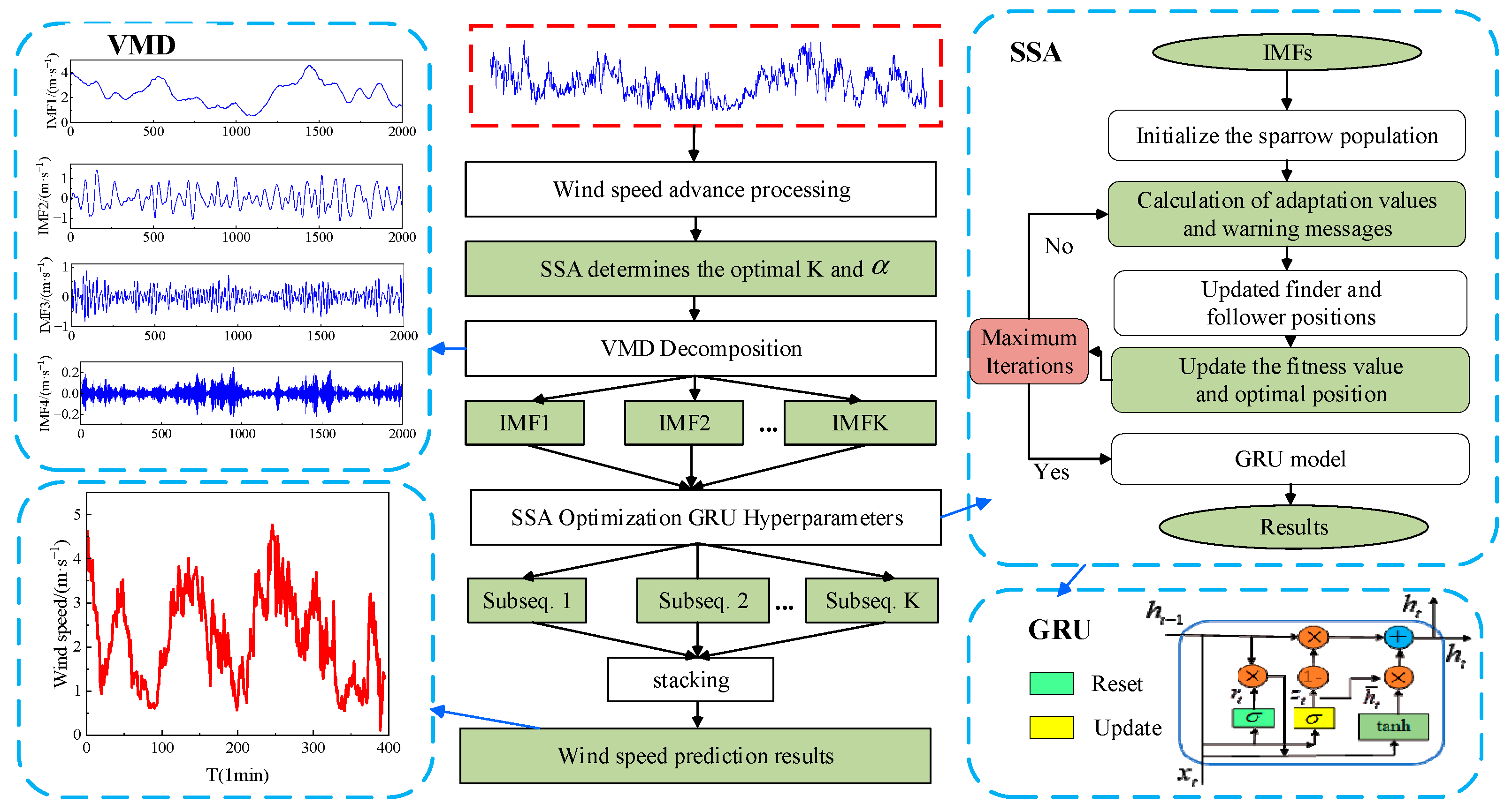
2.1. Overall Framework

This study developed several hybrid optimized models for predicting wind speed. The methodology for creating these models includes three primary steps, namely (1) decomposing the original wind speed sequence into multiple components using WT and VMD; (2) utilizing various neural networks, including GRU, LSTM [17], SSA–LSTM, and SSA–GRU, to predict each component individually [18]; and (3) linearly combining the predicted values from each component to generate the final wind speed prediction. Based on this methodology, eight prediction models were developed: WT–LSTM, WT–GRU, WT–SSA–LSTM, WT–SSA–GRU, VMD–LSTM, VMD–GRU, VMD–SSA–LSTM, and VMD–SSA–GRU. The framework of these hybrid optimized prediction models is illustrated in Figure 1. To evaluate the effectiveness of the hybrid model in predicting wind speed, several single models were also established for comparison, including back propagation (BP), support vector machines (SVMs), CNNs [19], LSTM, and GRU neural networks [20].

2.2. VMD

As mentioned when discussing the advantages of the VMD in the Introduction, VMD is regarded as a fully non-recursive adaptive signal decomposition method [21]. By preprocessing the original wind speed data, VMD decomposes the non-stationary wind speed sequence into several submodal time sequences, which is essential for enhancing the accuracy of wind speed predictions. In VMD, the decomposition order, K, must be predetermined. Decomposing the non-stationary wind speed sequence, x(t), into a K-order VMD is treated as a constrained optimization variational problem that aims to decompose the input signal x(t) into K modal functions. The VMD signal decomposition process involves the following steps:

$$\left\{\begin{array}{l}\underset{\left\{u_k\right\},\left\{w_k\right\}}{\min }{{\displaystyle \sum _k‖{\partial }_t\left[\left(\delta \left(t\right)+\frac{j}{\pi t}\right)*u_k\left(t\right)\right]e^{-j{\omega }_{k}t}‖}}^2\\ s.t.{\displaystyle \sum _k{u}_k(t)=x(t)}\end{array}\right.,$$

(1)

where $u_k$ and $w_k$ represent the k-th modal component and its central frequency, respectively; $\delta \left(t\right)$ denotes the Dirac delta function; and * indicates the convolution operation. By introducing the quadratic penalty factor $\alpha$ and Lagrange operator $\beta$, Equation (1) is transformed into an augmented Lagrangian equation, as expressed in Equation (2). x(t) represents the original wind speed data, and this constrained optimization problem is transformed into an unconstrained optimization problem for the solution.

$$\begin{array}{l}L\left(\left\{u_k\right\},\left\{w_k\right\},\lambda \right)=\alpha {{\displaystyle \sum _{k=1}^K‖{\partial }_t\left[\left(\delta \left(t\right)+\frac{j}{\pi t}\right)*u_k\left(t\right)\right]e^{-j{\omega }_{k}t}‖}}_2^2\\ +{‖x(t)-{\displaystyle \sum _{k=1}^K{u}_k(t)}‖}_2^2+\left(\lambda (t),x(t)-{\displaystyle \sum _{k=1}^K{u}_k(t)}\right)\end{array}$$

(2)

The solution to the constrained variational Equation (2) is then approached by solving the saddle-point problem of the augmented Lagrangian equation. The saddle point is determined by alternately updating each modal component and its central frequency using the method of multipliers in the alternating direction. The updated formulas are detailed in the subsequent equations.

$${\widehat{u}}_k^{n+1}(w)={\displaystyle \frac{\widehat{x}(w)-{\displaystyle \sum _{i\ne k}{\widehat{u}}_i(w)+\frac{\widehat{\lambda }(w)}{2}}}{1+2\alpha {(w-w_k)}^2}}$$

(3)

$$w_k^{n+1}={\displaystyle \frac{{\displaystyle {\int }_0^{\infty }w{\left|{\widehat{u}}_k(w)\right|}^{2}dw}}{{\displaystyle {\int }_0^{\infty }{\left|{\widehat{u}}_k(w)\right|}^{2}dw}}}$$

(4)

where ${\widehat{u}}_k^{n+1}(w)$, $\widehat{x}(w)$, ${\widehat{u}}_i(w)$, and $\widehat{\lambda }(w)$ represent the Fourier transforms of $u_k^{n+1}(t)$, $x(t)$, $u_i(t)$, and $\lambda (t)$, respectively; w denotes the frequency; and n indicates the iteration count.

2.3. GRU Neural Network Model

The GRU model enhances the LSTM neural network model and is increasingly utilized in time series prediction research [22,23]. The GRU model is described by the computational formula in Equation (5), has fewer training parameters compared to the LSTM model, and offers significant advantages in terms of convergence speed and prediction accuracy. The GRU neural network consists of two gate structures: the reset gate and the update gate. The reset gate manages the integration of previous and current input information, while the update gate regulates the extent to which past information is forgotten and current information is retained. Figure 2 illustrates the internal structural units of the GRU neural network.

$$\left\{\begin{array}{c}{r}_t=\sigma \left(W_r·\left[h_{t-1},x_t\right]\right)\hfill \\ z_t=\sigma \left(W_z·\left[h_{t-1},x_t\right]\right)\hfill \\ {\tilde{h}}_t=\tanh \left(W_{\tilde{h}}·\left[r_t\times h_{t-1},x_t\right]\right)\hfill \\ h_t=\left(1-z_t\right)\times h_{t-1}+z_t\times {\tilde{h}}_t\hfill \end{array}\right.$$

(5)

where $x_t$ represents the input at the current time step; $h_{t-1}$ represents the state at the previous time step; W_r represents the weight matrix of the reset gate; W_Z represents the weight matrix of the update gate; r_t indicates the reset gate; z_t indicates the update gate; ${\tilde{h}}_t$ denotes the candidate’s hidden information at the current time step; h_t represents the output of the current network layer; $\sigma$ denotes the sigmoid activation function; and tanh denotes the hyperbolic tangent activation function.

2.4. Sparrow Optimization Algorithm

The sparrow optimization algorithm is a swarm intelligence technique that facilitates both global and local searches [24]. In deep learning, this algorithm optimizes the weights and thresholds of neural networks, which significantly reduces the training time and enhancement performance. The algorithm models the foraging behavior of sparrows by categorizing them into explorers, followers, and scout alarmists. Explorers identify foraging directions and areas for the group, followers primarily track the explorers to forage, and scout alarmists issue alerts upon detecting threats, triggering anti-predatory behavior in the population [25].

$$X_{ij}^{t+1}=\left\{\begin{array}{cc}{X}_{ij}^t\exp ({\displaystyle \frac{-i}{\alpha D_{\max }}})\hfill & R_2<S_T\hfill \\ X_{ij}^t+QL\hfill & R_2\ge S_T\hfill \end{array}\right.$$

(6)

where $X_{ij}$ represents the position information of the i-th sparrow in the j-th dimension; $j=1,2,3,\dots d$, d denotes the dimensionality of the variable to be optimized; t represents the current iteration count; $\alpha (\alpha \in [0,1])$ represents a random number; $D_{\max }$ denotes the maximum number of iterations; $R_2\left(R_2\in [0,1]\right)$ represents the warning value; $S_T$ represents the safety value; $Q$ represents random numbers following a normal distribution; and $L$ represents a matrix with all elements equal to 1 and of size $1\times d$. When $R_2<S_T$, the environment is deemed safe and the search continues; otherwise, scout alarmists signal a warning, which prompts a rapid retreat of the sparrow population. The position update for the followers mirrors that of the explorers. If followers observe and decide to compete with the explorers, their positions are updated using the following equation:

$$X_{ij}^{t+1}=\left\{\begin{array}{cc}Q\exp ({\displaystyle \frac{X_{worst}^t-X_{ij}^t}{\alpha D_{\max }}})\hfill & \hfill \mathrm{i}>\frac{n}{2}\\ X_P^{t+1}+\left|X_{ij}^t-X_p^{t+1}\right|A^{+}L\hfill & \hfill \mathrm{i}\le \frac{n}{2}\end{array}\right.$$

(7)

where $X_p$ represents the optimal position of the discoverer; $X_{worst}$ denotes the worst position; and A denotes a matrix of size 1 × d, where each element is within the range of {−1,1} and satisfies A⁺ = A^T(AA^T)⁻¹; and i > n/2 represents that the i-th joiner with a lower fitness value is in a hungry state as it does not procure food. If followers observe and decide to compete with the explorers, their positions are updated using the following equation:

$$X_{ij}^{t+1}=\left\{\begin{array}{cc}{X}_{best}^t+\beta \left|X_{ij}^t-X_{best}^t\right|\hfill & f_{\mathrm{i}}>f_{\mathrm{g}}\hfill \\ X_{ij}^t+K\left|\frac{X_{ij}^t-X_{worst}^t}{\left(f_i-f_w\right)+\epsilon }\right|\hfill & f_{\mathrm{i}}=f_{\mathrm{g}}\hfill \end{array}\right.$$

(8)

where $X_{best}^t$ represents the current optimal position; $\beta$ serves as the step-size control parameter; $f_i$, $f_g$, and $f_w$ denote the current fitness, best fitness, and worst fitness, respectively; K denotes a random number in the range [−1, 1]; and $\epsilon$ denotes a constant to avoid division by zero.

The computation process of the sparrow optimization algorithm is illustrated in Figure 3 and includes the following steps: (1) input the initial wind speed sequence; (2) initialize key parameters such as sparrow population size, initial positions, and best fitness values; (3) apply Equations (6)–(8) to compute the position of each sparrow, update the fitness values and the best position of the explorer, and review if the termination conditions are met; (4) if termination conditions are met, output the optimal weights and thresholds, and otherwise, repeat the process starting from step (2); (5) finally, output the optimal hyperparameters.

2.5. Adaptive VMD–SSA–GRU Model

This study introduces a novel method for predicting short-term wind speed using the VMD–SSA–GRU model, which is enhanced by the sparrow optimization algorithm. The VMD–SSA–GRU neural network functions in the following manner: Initially, the parameters K and α of VMD are optimized using SSA. Subsequently, the original non-stationary signal is decomposed into subsequences of different frequency modal components through adaptive VMD. Given that the prediction accuracy of the GRU model is significantly influenced by its hyperparameters, SSA is also employed to optimize these parameters. The optimized hyperparameters are then integrated into the GRU to predict each intrinsic mode function (IMF) component reconstructed in the phase space. The results from each component are aggregated to finalize the prediction. This process is illustrated in Figure 3.

2.6. SSA Performance Test

To evaluate the efficiency of the SSA, this section compares the optimization performance of four different algorithms across eight mathematical problems. The test functions include two unimodal functions that exhibit a single extremum point within their domain; one multimodal function that contains multiple peak points within its domain and is used to assess the global search capability and the ability to escape from local optima of the algorithms; and three fixed-dimensional multimodal functions that possess a set number of local extremum points within their domain. The details of these test functions are provided in the accompanying table.

The comparison involves five optimization algorithms: whale optimization algorithm (WOA), firefly swarm optimization algorithm (FSO), bald eagle search optimization algorithm (BES), and beluga whale optimization (BWO). To ensure a fair comparison, each algorithm was configured with a population size of 50 and a maximum of 1000 iterations. The means and standard deviations of 30 optimization trials were calculated as performance metrics. The test functions used in the optimization trials are listed in

Table 2. Test Functions.

Type	Number	Function	fmin
Unimodal Functions	F1	$F_1(x)={\displaystyle \sum _{i=1}^n{x}_i^2}$	0
	F2	$F_5(x)={\displaystyle \sum _{i=1}^{n-1}\left[100{\left(x_{i+1}-x_i^2\right)}^2+{\left(x_i-1\right)}^2\right]}$	0
Unimodal Functions	F3	$F_8(x)={\displaystyle {\sum }_{i=1}^n-x_i\sin \left(\sqrt{\left|x_i\right|}\right)}$	−2.09 × 103
Fixed Dimension	F4	$F14(X)={\left({\displaystyle \frac{1}{500}}+{\displaystyle {\sum }_{j=1}^{25}\frac{1}{j+{\displaystyle {\sum }_{i=1}^2{\left(x_i-a_{ij}\right)}^6}}}\right)}^{-1}$	1
	F5	$\begin{array}{l}{F}_{18}(x)=\left[1+{\left(x_1+x_2+1\right)}^2\left(19-14x_1+3x_1^2-14x_2+6x_1{x}_2+3x_2^2\right)\right]\hfill \\ \hspace{1em}\times \left[30+{\left(2x_1-3x_2\right)}^2\times \left(18-32x_1+12x_1^2+48x_2-36x_1{x}_2+27x_2^2\right)\right]\hfill \end{array}$	3
	F6	$F_{23}(x)=-{\displaystyle \sum _{i=1}^{10}{\left[\left(X-a_i\right){\left(X-a_i\right)}^T+c_i\right]}^{-1}}$	−10.5363

. The results presented in

Table 3. Comparison of Results from Different Algorithmic Solutions.

Number	Index	SSA	WOA	TSO	BES	BWO
F1	Ave	3.85 × 10−169	1.84 × 10−169	0.00	0.00	0.00
	Std	0.00	0.00	0.00	0.00	0.00
F2	Ave	2.93 × 10−91	2.66 × 10	1.52 × 10−4	3.15 × 10−3	5.23 × 10−255
	Std	1.60 × 10−90	3.77 × 10−1	4.28 × 10−4	4.22 × 10−3	0.00
F3	Ave	−2.67 × 103	−1.20 × 104	−1.26 × 104	−8.16 × 103	3.30 × 10−5
	Std	2.66 × 10−4	9.25 × 102	1.38 × 10−5	1.24 × 103	2.56 × 10−5
F4	Ave	9.98 × 10−1	1.56	9.98 × 10−1	3.80	4.44 × 10−16
	Std	0.00	1.85	1.91 × 10−16	4.59	0.00
F5	Ave	3.00	3.00	3.00	3.00	1.64 × 10−25
	Std	1.24 × 10−15	1.14 × 10−6	1.19 × 10−15	1.26 × 10−15	2.32 × 10−25
F6	Ave	−1.05 × 10	−9.43	−1.05 × 10	−8.91	−1.04 × 10
	Std	8.73 × 10−16	2.34	2.09 × 10−15	2.52	3.17 × 10−6

indicate that for unimodal functions, the performance metrics of the algorithms are relatively similar. However, for multimodal and composite functions, SSA demonstrates superior optimization effectiveness compared to the other algorithms.

3. Wind Speed Prediction Evaluation

3.1. Model Evaluation Metrics

To assess the predictive accuracy of various models, three widely used evaluation metrics were employed to quantify the performances of all of the models used herein: root-mean-square error (RMSE), mean absolute error (MAE), and mean absolute percentage error (MAPE), as defined by the following formulas [26].

$$RMSE=\sqrt{{\displaystyle \frac{1}{n}}{\displaystyle {\sum }_{i=1}^n{(x_i-{\widehat{x}}_i)}^2}}$$

(9)

$$MAE={\displaystyle \frac{1}{n}}{\displaystyle {\sum }_{i=1}^n\left|x_i-{\widehat{x}}_i\right|}$$

(10)

$$MAPE={\displaystyle \frac{1}{n}}{\displaystyle {\sum }_{i=1}^n\left|\frac{x_i-{\widehat{x}}_i}{x_i}\right|}\times 100\%$$

(11)

where $n$ represents the total number of samples in the predictive model; ${\widehat{x}}_i$, $x_i$, and ${\overline{x}}_i$ denote the predicted value, actual value, and mean value of all samples for the $i$-th sample point, respectively.

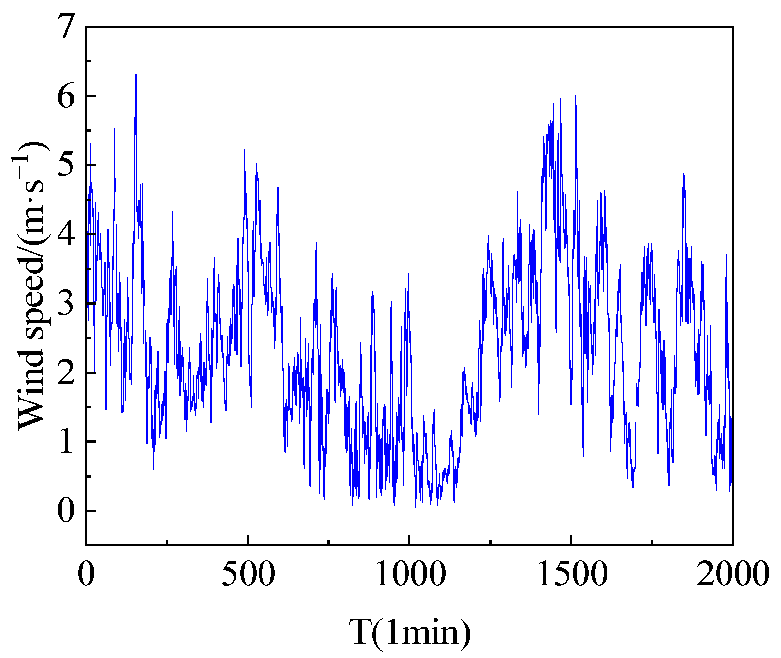
3.2. Original Wind Speed

To verify the reliability of the adaptive VMD–SSA–GRU model, this study employed measured wind speed data from a meteorological station near a bridge site in the southwest region as verification samples, as documented in reference [27]. The wind speed sequence is depicted in Figure 4. The sequence consisted of 2000 data points, sampled at one-minute intervals. The dataset was divided into a training set, comprising 80% of the total samples (data points 1–1600), and a test set, comprising the remaining 20% (data points 1601–2000). The Kwiatkowski–Phillips–Schmidt–Shin (KPSS) test was employed as a statistical test to estimate the non-stationary characteristic of the measured wind speed [28]. According to the KPSS test, the KPSS value is 0.01, which is greater than 0, and implies that the measured wind speed is non-stationary. If necessary, the original wind speed dataset can be downloaded as supplementary information from the official website. Different from the DL network in other fields, all of the input and output parameters are identical in the proposed model for wind speed prediction. The five-step prediction method is adopted for all of the involved models. Specifically, the first five wind speed data points are used as input parameters, and the last data points are used as the expected value of the output parameter [29].

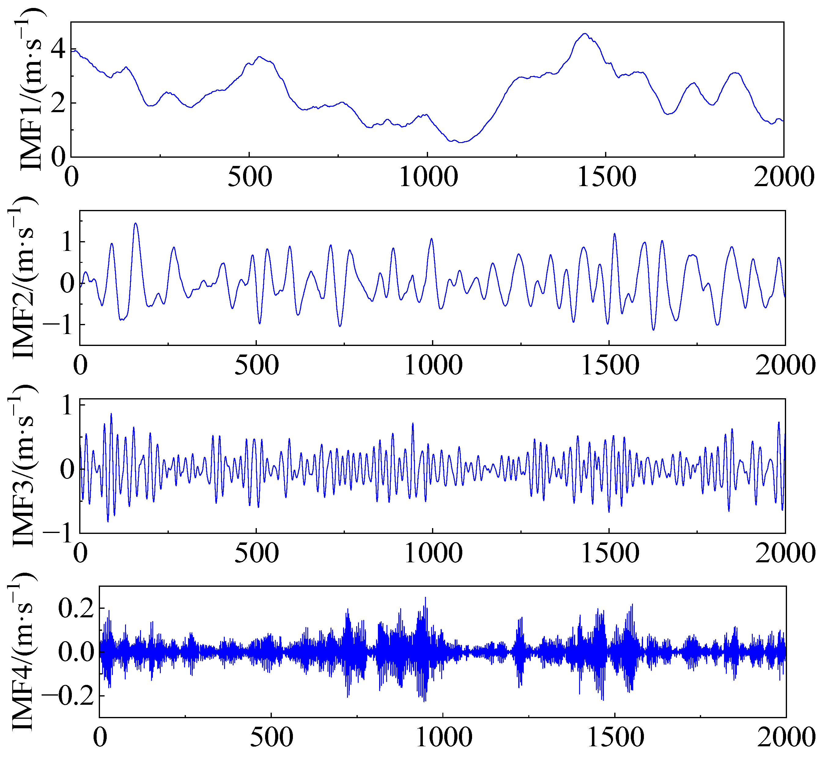
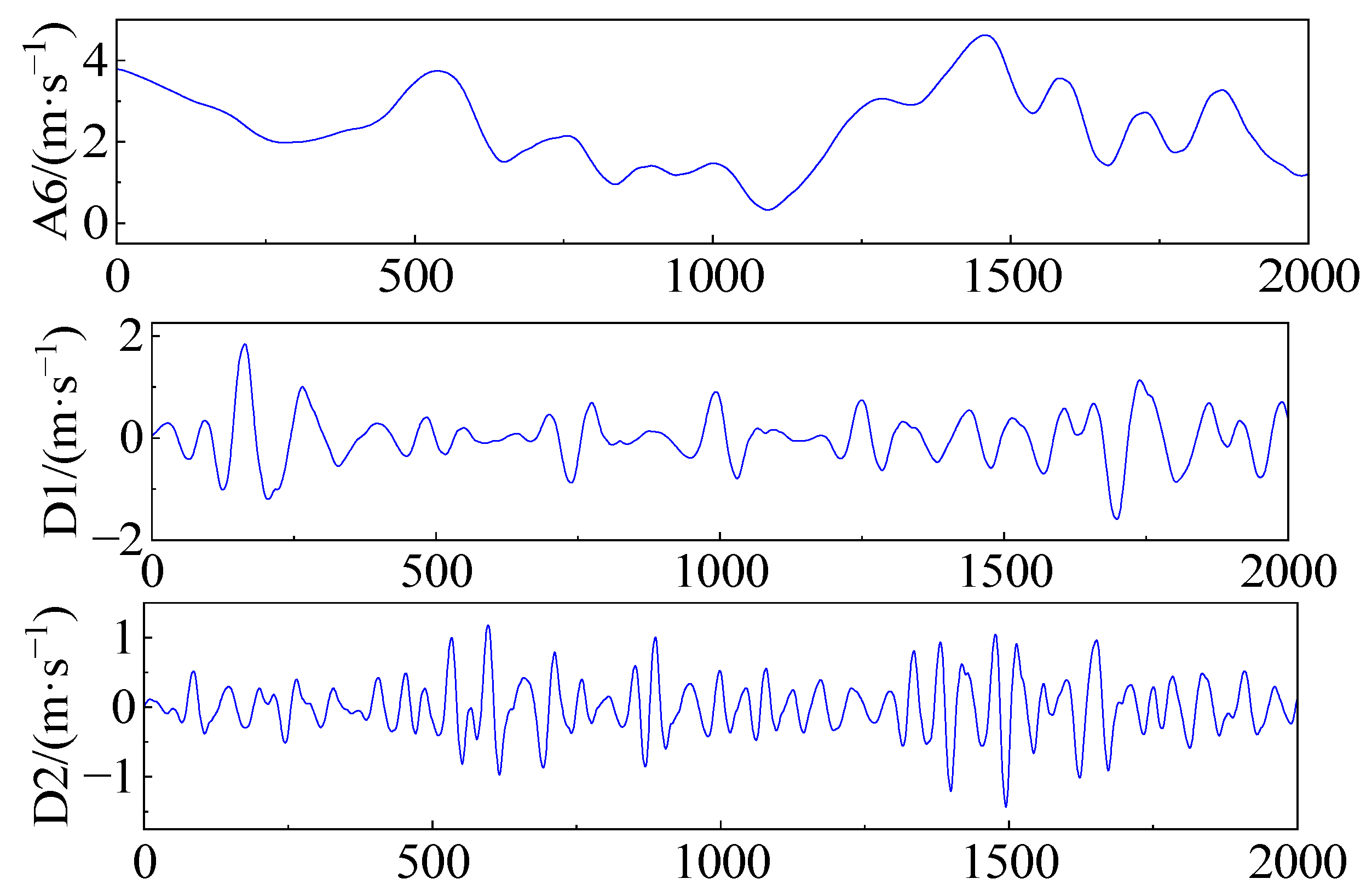
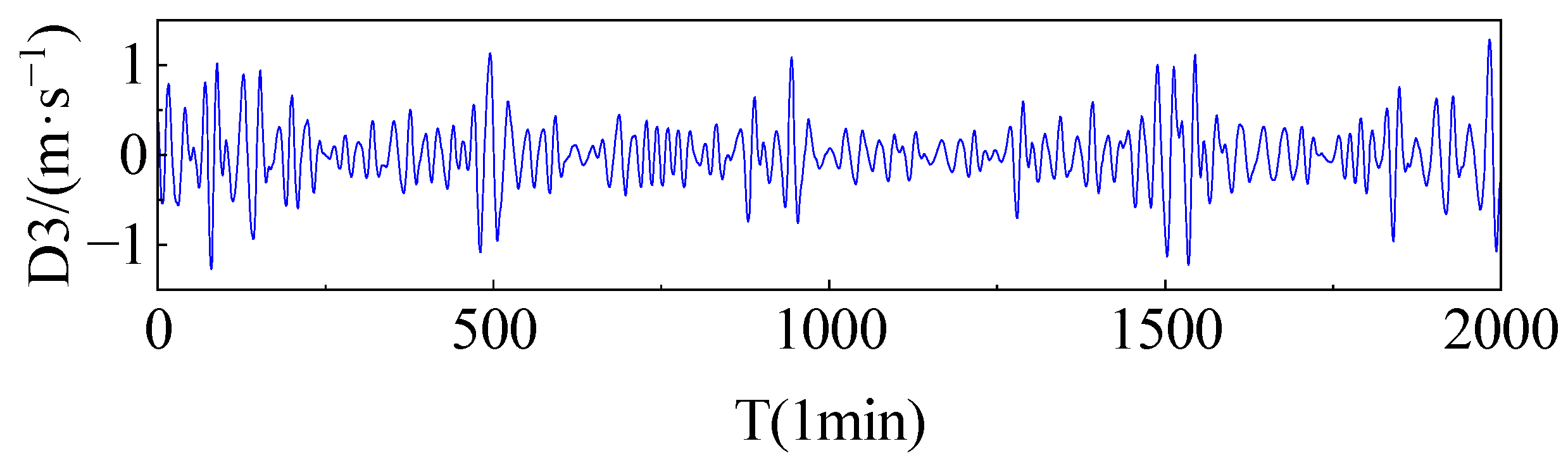
3.3. Wind Speed Decomposition

The VMD method adaptively performs a frequency-domain division of signals and effectively isolates IMFs. This transformation facilitates the management of non-stationary and highly nonlinear time series by segregating them into subsequences that contain multiple different frequency scales with relatively stable characteristics. The parameters K and α in the VMD algorithm are crucial as they significantly influence the accuracy and stability of the decomposition results.

Specifically, a small K value may result in multiple signal components being merged into a single mode, which can obscure the true features of the original signal in the decomposition results. Conversely, a large K value might lead to the decomposition of one component into multiple modes, which complicates the subsequent analyses. Although a small penalty parameter α may retain more frequency components, it also includes unwanted noise in the decomposition results. A large α value might eliminate useful frequency components, thereby diminishing the accuracy of the results. Therefore, selecting an appropriate combination of K and α values is essential for optimizing the performance of the VMD algorithm.

This study employed the validated SSA to optimize the parameters K and α of the VMD algorithm. The population size for the SSA was set at 30, with a maximum iteration limit of 10. The fitness function utilized was the mean envelope spectrum kurtosis, calculated using Equation (12). The optimization ranges for K and α were set to [2, 10] and [200, 4000], respectively, whereas other parameters remained at their default settings. After iterative optimization, the optimal values for K and α were determined to be 7 and 2600, respectively. The first four IMF components from the VMD are illustrated in Figure 5, where IMF1 represents the low-frequency component, indicating the primary trend in the wind speed signal, and IMF4 captures the high-frequency component, reflecting the transient local characteristics of the wind speed. From Figure 5, IMF1 presents the global time-varying trend for the mean value of the measured wind speed. The time-varying mean value further illustrates the non-stationary feature of the dataset used.

$$\left\{\begin{array}{l}{K}_{\mathrm{E}}={\displaystyle \frac{\mathrm{E}{\left(E_x-{\tau }_{\mathrm{E}}\right)}^4}{{\mu }_{\mathrm{E}}^4}},\hfill \\ K_{\mathrm{ES}}={\displaystyle \frac{\mathrm{E}{\left(E{S}_x-{\tau }_{\mathrm{ES}}\right)}^4}{{\mu }_{\mathrm{ES}}^4}}.\hfill \end{array}\right.$$

(12)

where $K_{\mathrm{E}}$ represents the signal envelope steepness; E denotes the mathematical expectation; $E_x$ denotes the signal after the Hilbert transform; ${\tau }_{\mathrm{E}}$ indicates the mean value of $E_x$; ${\mu }_{\mathrm{E}}^4$ represents the standard deviation of Ex; $K_{\mathrm{ES}}$ represents the envelope spectrum steepness; $E{S}_x$ denotes the discrete Fourier transform of the envelope signal; ${\tau }_{\mathrm{ES}}$ denotes the mean value of $E{S}_x$; and ${\mu }_{\mathrm{ES}}^4$ represents the standard deviation of $E{S}_x$.

Moreover, to evaluate the effectiveness of the VMD method in improving the accuracy of wind speed predictions, this study utilized the WT method as a comparative baseline. The wind speed data were decomposed using built-in wavelet decomposition functions in MATLAB, selecting the db6 wavelet base and Level 6 decomposition, in alignment with the existing literature [5]. This decomposition resulted in one approximate component (A6) and six detail components (D1–D6), with the first four components illustrated in Figure 6. Similar to IMF1, component A6 also presents the non-stationary feature of the measured wind speed used in the study.

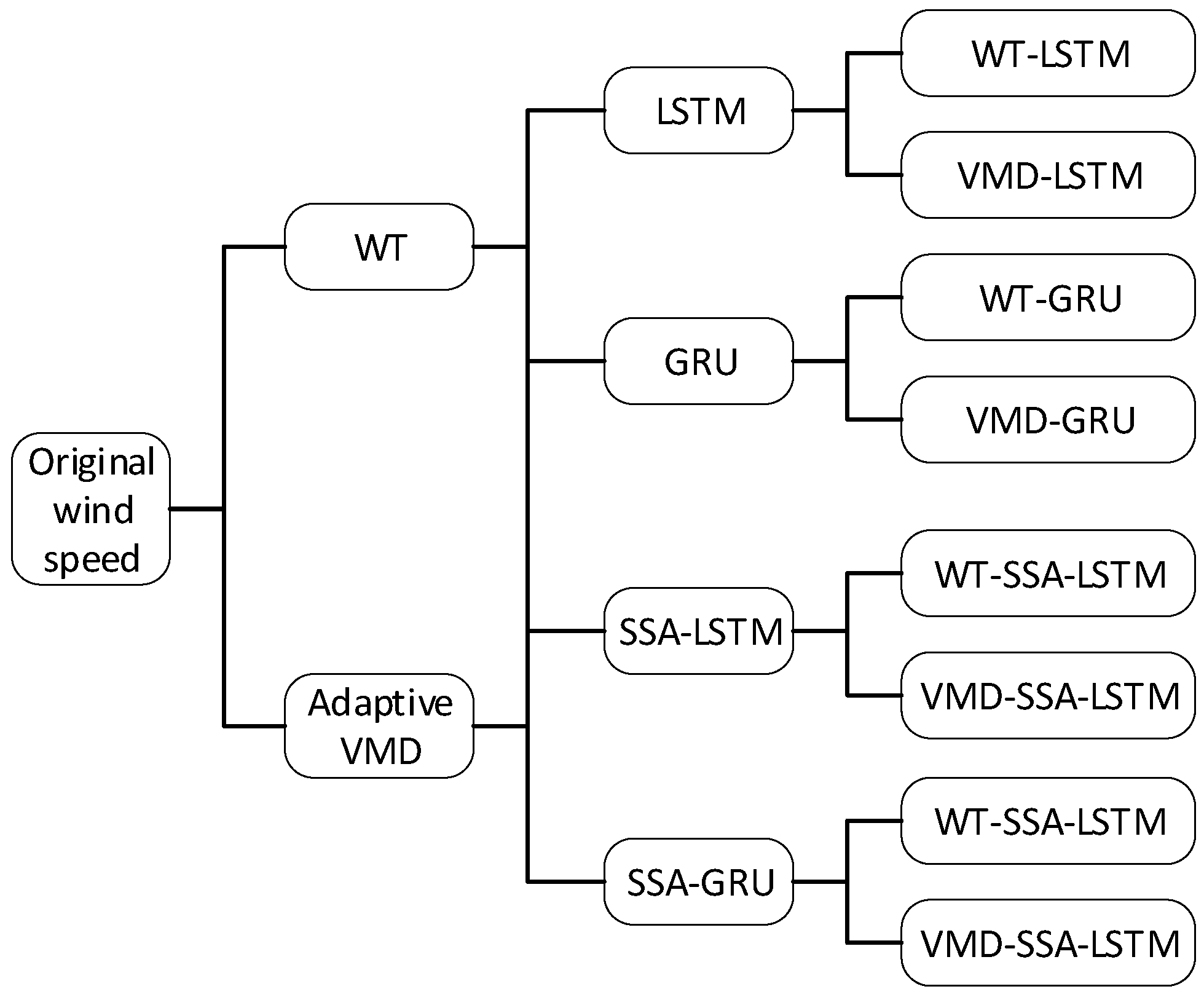
3.4. Single Model Prediction Performance

The study further examined the influence of a hybrid optimization model on the accuracy of wind speed predictions by comparing the performance of various single neural network models, including BP, CNN, SVM, LSTM, and GRU networks. Figure 7 displays a comparison between the predicted and actual wind speeds across these networks, whereas Figure 8 depicts that most neural networks closely match the predicted values to the actual values. However, the CNN model demonstrated a poor fit, characterized by a noticeable lag, owing to its tendency to capture local dependencies in sequences. This leads to significant prediction errors in wind speed time series that exhibit non-stationary characteristics and temporal dependencies.

Among the single neural network models evaluated, as listed in

Table 4. Prediction error of single neural networks.

Prediction Model	BP	CNN	SVM	LSTM	GRU
RMSE/(m·s−1)	0.36953	0.41718	0.36951	0.36797	0.3679
MAE/(m·s−1)	0.28301	0.32404	0.27949	0.28185	0.28109
MAPE/%	10.8521	12.5183	10.9059	10.9466	10.8986

, the SVM, LSTM, and GRU models achieved RMSEs of 0.36951, 0.36797, and 0.3679 m/s, respectively, indicating their high accuracy in approximating actual wind speeds. As variants of recurrent neural networks, the LSTM and GRU models are particularly effective at capturing long-range dependencies in time series data, providing them with an advantage in handling time-dependent series.

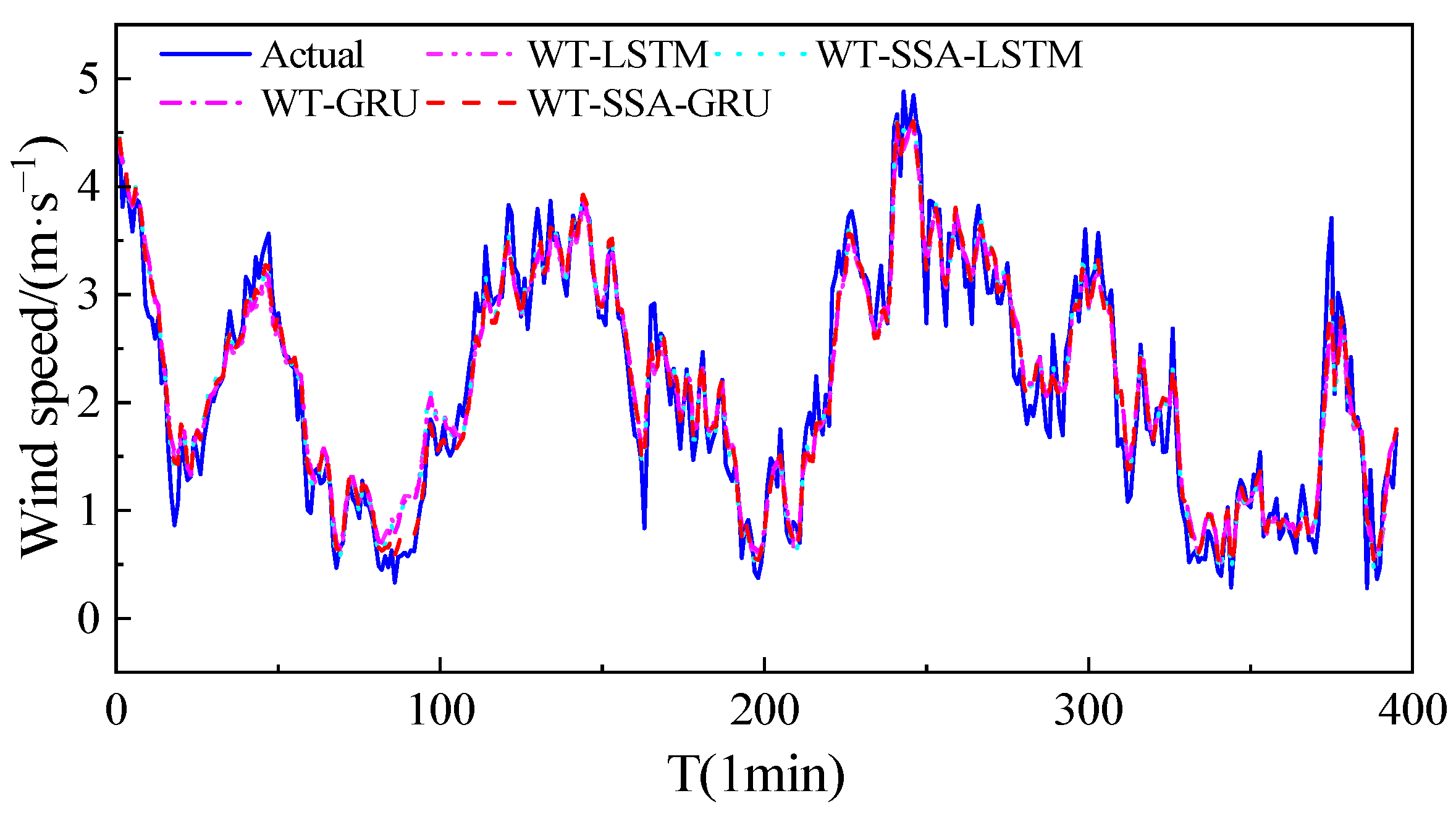
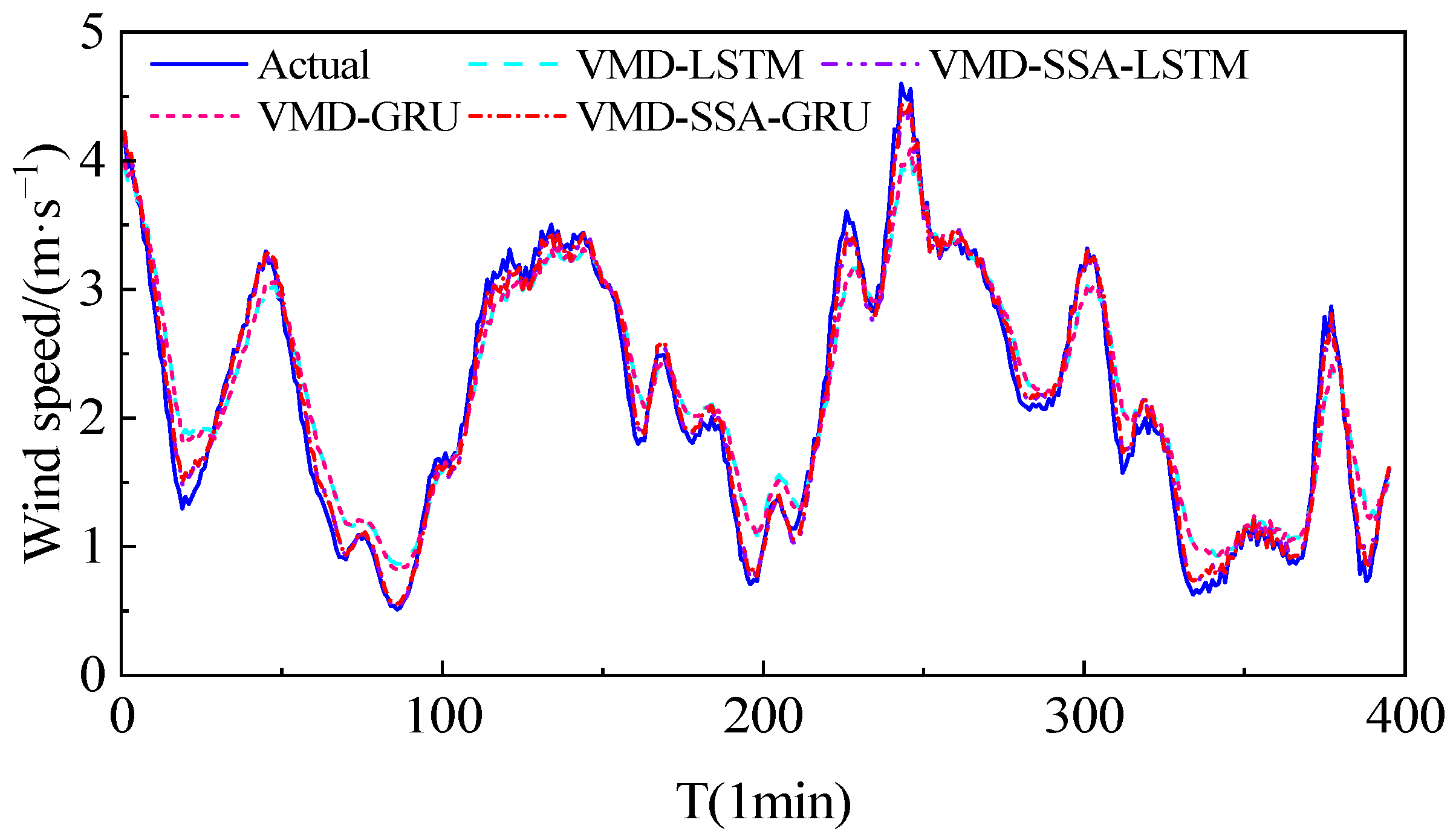
3.5. Hybrid Model Predictive Performance

The performance of a model is significantly influenced by the selection of hyperparameters. Optimizing these parameters can improve the model’s accuracy, generalization capability, and training efficiency. For the GRU model, the number of layers, learning rate, and maximum number of iterations were optimized using a validated efficient SSA, with specific ranges and results detailed in

Table 5. SSA-optimized GRU hyperparameters.

Hyperparameters	Optimization Range	Optimal Value
GRU Network Layers	[20, 400]	244
Learning Rate	[0.0001, 0.2]	0.00198
Maximum Iterations	[20, 500]	338

. Similarly, the SSA-optimized LSTM hyperparameters are listed in

Table 6. SSA-optimized LSTM hyperparameters.

Hyperparameters	Optimization Range	Optimal Value
LSTM Network Layers	[20, 400]	308
Learning Rate	[0.0001, 0.2]	0.00115
Maximum Iterations	[20, 500]	269

. To evaluate the effectiveness and robustness of the proposed adaptive VMD–SSA prediction model, this study compared its predictive accuracy with various hybrid models, including WT–LSTM, WT–GRU, WT–SSA–LSTM, WT–SSA–GRU, VMD–LSTM, VMD–GRU, and VMD–SSA–LSTM.

Figure 8 presents a comparison of predicted versus actual values using the WT hybrid model. Figure 9 indicates that among the models, WT–SSA–GRU achieved the highest predictive accuracy, followed by WT–SSA–LSTM, with WT–GRU and WT–LSTM showing lower performances. According to

Table 7. Prediction error of hybrid models.

Models	RMSE/(m·s−1)	MAE/(m·s−1)	MAPE/%
WT–GRU	0.26098	0.20602	7.6101
WT–SSA–GRU	0.22181	0.17218	6.5966
WT–LSTM	0.27153	0.21287	8.0096
WT–SSA–LSTM	0.22679	0.17691	6.6146
VMD–GRU	0.25171	0.20403	7.5058
VMD–SSA–GRU	0.10018	0.080954	3.1461
VMD–LSTM	0.26179	0.20469	7.9107
VMD–SSA–LSTM	0.13428	0.087361	3.2432

, the RMSE values for WT–SSA–GRU, WT–SSA–LSTM, WT–GRU, and WT–LSTM were 0.22181, 0.22679, 0.26098, and 0.27153 m/s, respectively. The WT–SSA–GRU model demonstrated a 15.0% improvement in predictive accuracy over the WT–GRU model. The non-recursive nature of VMD and its effectiveness in extracting the central frequency of signals contribute to its superior ability to capture dynamic signal features, resulting in a 3.9% improvement in predictive accuracy over the WT–GRU and WT–LSTM models.

Figure 9 compares the predicted and actual values of the VMD hybrid models. As observed in Figure 9, the predictive performance of the VMD–SSA–LSTM and VMD–SSA–GRU models surpasses that of the VMD–LSTM and VMD–GRU models in terms of wind speed trend changes and extreme wind speed values. The RMSE values for the VMD–SSA–GRU model show reductions of 25.3%, 60.2%, and 61.7% compared to the VMD–SSA–LSTM, VMD–GRU, and VMD–LSTM models, respectively.

Table 4 and Table 7 provide a comparison of the predictive performance of single and hybrid models on wind speed. The data show that hybrid neural networks surpass single neural networks, with the integration of the sparrow optimization algorithm further improving prediction accuracy. The WT–SSA–GRU model yielded RMSE, MAE, and MAPE values of 0.22181, 0.17218, and 6.5966%, respectively, representing decreases of 39.7%, 38.7%, and 39.5% compared to the GRU prediction model. Similarly, the VMD–SSA–GRU model recorded RMSE, MAE, and MAPE values of 0.10018, 0.080954, and 3.1461%, respectively, reflecting reductions of 72.7%, 71.2%, and 71.1% compared to the GRU neural network. These results confirm that the VMD–SSA–GRU model achieves the highest predictive accuracy.

4. Conclusions

Predicting wind speed is essential for the real-time scheduling of wind power grid-connected systems. This study introduces a novel method for short-term wind speed prediction using the VMD–SSA–GRU model. For comparative analysis, various hybrid models including WT–LSTM, WT–GRU, WT–SSA–LSTM, WT–SSA–GRU, VMD–LSTM, VMD–GRU, and VMD–SSA–LSTM, as well as single models such as BP, CNNs, SVMs, LSTM, and GRUs were evaluated using data from a meteorological station near a specific bridge.

The comparative analysis indicated that the SSA outperforms other optimization algorithms in global search capability and in avoiding local optima in various mathematical problems. By efficiently optimizing the K and α values of the VMD algorithm, the SSA enhances the decomposition accuracy and stability of the wind speed signals. Additionally, the optimization of hyperparameters such as the number of layers, learning rate, and maximum iteration times in the GRUs by the SSA significantly improves the prediction accuracy.

The adaptive VMD–SSA–GRU model proposed in this research demonstrated the highest predictive accuracy among the models tested. It outperformed adaptive VMD and WT models in handling non-stationary wind speed sequences by more effectively extracting frequency-domain characteristics of wind speed signals. Furthermore, it exhibited superior predictive performance compared to both hybrid optimization decomposition models and single models. What is noteworthy is that the accuracy of the proposed VMD-SSA-GRU model was validated through the short-term wind speed prediction. The estimation should be investigated further in the medium and long terms, and studying its applicability in different topographies is our future endeavor.

References

1. Yu, C.; Li, Y.; Bao, Y.; Tang, H.; Zhai, G. A novel framework for wind speed prediction based on recurrent neural networks and support vector machine. Energy Convers. Manag. 2018, 178, 137–145. [Google Scholar] [CrossRef]
2. Yuan, X.; Chen, C.; Jiang, M.; Yuan, Y. Prediction interval of wind power using parameter optimized Beta distribution-based LSTM model. Appl. Soft Comput. 2019, 82, 105550. [Google Scholar] [CrossRef]
3. Zhang, Z.D.; Ye, L.; Qin, H.; Liu, Y.; Wang, C.; Yu, X.; Yin, X.; Li, J. Wind speed prediction method using shared weight long short-term memory network and gaussian process regression. Appl. Energy 2019, 247, 270–284. [Google Scholar] [CrossRef]
4. Aasim, S.S.N.; Singh, S.N.; Mohapatra, A. Repeated wavelet transform based Arima model for very short-term wind speed forecasting. Renew. Energy 2019, 136, 758–768. [Google Scholar] [CrossRef]
5. Wang, J.; Li, Z. Wind speed interval prediction based on multidimensional time series of Convolutional Neural Networks. Eng. Appl. Artif. Intell. 2023, 121, 105987. [Google Scholar] [CrossRef]
6. Memarzadeh, G.; Keynia, F. A new short-term wind speed forecasting method based on fine-tuned LSTM neural network and optimal input sets. Energy Convers. Manag. 2020, 213, 112824. [Google Scholar] [CrossRef]
7. Zhang, Y.-M.; Wang, H. Multi-head attention-based probabilistic CNN-BiLSTM for day-ahead wind speed forecasting. Energy 2023, 278, 127865. [Google Scholar] [CrossRef]
8. Wu, J.; Li, N.; Zhao, Y.; Wang, J. Usage of correlation analysis and hypothesis test in optimizing the gated recurrent unit network for wind speed forecasting. Energy 2022, 242, 122960. [Google Scholar] [CrossRef]
9. Jiang, W.; Lin, P.; Liang, Y.; Gao, H.; Zhang, D.; Hu, G. A novel hybrid deep learning model for multi-step wind speed forecasting considering pairwise dependencies among multiple atmospheric variables. Energy 2023, 285, 129408. [Google Scholar] [CrossRef]
10. Jiang, W.; Liu, B.; Liang, Y.; Gao, H.; Lin, P.; Zhang, D.; Hu, G. Applicability analysis of transformer to wind speed forecasting by a novel deep learning framework with multiple atmospheric variables. Appl. Energy 2024, 353, 122155. [Google Scholar] [CrossRef]
11. Liu, H.; Mi, X.; Li, Y. Smart deep learning based wind speed prediction model using wavelet packet decomposition, convolutional neural network and convolutional long short term memory network. Energy Convers. Manag. 2018, 166, 120–131. [Google Scholar] [CrossRef]
12. He, X.H.; Duan, Q.C.; Yan, L. Short-term wind speed probability prediction based on DeepAR. J. Railw. Res. 2023, 45, 152–160. [Google Scholar]
13. Yan, Y.; Wang, X.; Ren, F.; Shao, Z.; Tian, C. Wind speed prediction using a hybrid model of EEMD and LSTM considering seasonal features. Energy Rep. 2022, 8, 8965–8980. [Google Scholar] [CrossRef]
14. Zhao, Z.; Yun, S.; Jia, L.; Guo, J.; Meng, Y.; He, N.; Li, X.; Shi, J.; Yang, L. Hybrid VMD-CNN-GRU-based model for short-term forecasting of wind power considering spatio-temporal features. Eng. Appl. Artif. Intell. 2023, 121, 105982. [Google Scholar] [CrossRef]
15. Peng, S.; Zhu, J.; Wu, T.; Yuan, C.; Cang, J.; Zhang, K.; Pecht, M. Prediction of wind and PV power by fusing the multi-stage feature extraction and a PSO-BiLSTM model. Energy 2024, 298, 131345. [Google Scholar] [CrossRef]
16. Zhang, Y.G.; Chen, B.; Pan, G.F.; Zhao, Y. A novel hybrid model based on VMD-WT and PCA-BP-RBF neural network for short-term wind speed forecasting. Energy Convers. Manag. 2019, 195, 180–197. [Google Scholar] [CrossRef]
17. Shahid, F.; Zameer, A.; Muneeb, M. A novel genetic LSTM model for wind power forecast. Energy 2021, 223, 120069. [Google Scholar] [CrossRef]
18. Gao, X.; Guo, W.; Mei, C.; Sha, J.; Guo, Y.; Sun, H. Short-term wind power forecasting based on SSA-VMD-LSTM. Energy Rep. 2023, 9, 335–344. [Google Scholar] [CrossRef]
19. Guo, Z.; Yang, C.; Wang, D.; Liu, H. A novel deep learning model integrating CNN and GRU to predict particulate matter concentrations. Process Saf. Environ. Prot. 2023, 173, 604–613. [Google Scholar] [CrossRef]
20. Chen, G.; Tang, B.; Zeng, X.; Zhou, P.; Kang, P.; Long, H. Short-term wind speed forecasting based on long short-term memory and improved BP neural network. Int. J. Electr. Power Energy Syst. 2022, 134, 107365. [Google Scholar] [CrossRef]
21. Dragomiretskiy, K.; Zosso, D. Variational mode decomposition. IEEE Trans. Signal Process 2014, 62, 531–544. [Google Scholar] [CrossRef]
22. Yao, H.M.; Tan, Y.J.; Hou, J.C.; Liu, Y.; Zhao, X.; Wang, X. Short-term wind speed forecasting based on the EEMD-GS-GRU model. Atmosphere 2023, 14, 697. [Google Scholar] [CrossRef]
23. Zhang, G.W.; Liu, D. Causal convolutional gated recurrent unit network with multiple decomposition methods for short-term wind speed forecasting. Energy Convers. Manag. 2020, 226, 113500. [Google Scholar] [CrossRef]
24. Xue, J.; Shen, B. A novel swarm intelligence optimization approach: Sparrow search algorithm. Syst. Sci. Control Eng. 2020, 8, 22–34. [Google Scholar] [CrossRef]
25. Yue, Y.; Cao, L.; Lu, D.; Hu, Z.; Xu, M.; Wang, S.; Li, B.; Ding, H. Review and empirical analysis of sparrow search algorithm. Artif. Intell. Rev. 2023, 56, 10867–10919. [Google Scholar] [CrossRef]
26. Peng, Z.; Peng, S.; Fu, L.; Lu, B.; Tang, J.; Wang, K.; Li, W. A novel deep learning ensemble model with data denoising for short-term wind speed forecasting. Energy Convers. Manag. 2020, 207, 112524. [Google Scholar] [CrossRef]
27. He, X.H.; Shi, K.; Wu, T. An integrated structural health monitoring system for the Xijiang high-speed railway arch bridge. Smart Struct. Syst. 2018, 21, 611–621. [Google Scholar]
28. Hobijn, B.; Franses, P.H.; Ooms, M. Generalizations of the KPSS-test for stationarity. Stat. Neerl. 2004, 58, 483–502. [Google Scholar] [CrossRef]
29. Liu, H.; Mi, X.; Li, Y. Smart multi-step deep learning model for wind speed forecasting based on variational mode decomposition, singular spectrum analysis, LSTM network and ELM. Energy Convers. Manag. 2018, 159, 54–64. [Google Scholar] [CrossRef]
Figure 1. Frame diagram of hybrid forecast.
Processes 12 01741 g001
Figure 2. Structure of GRU neural network.
Processes 12 01741 g002
Figure 3. Algorithm flowchart.
Processes 12 01741 g003
Figure 4. Series of measured wind speed.
Processes 12 01741 g004
Figure 5. Results of VMD.
Processes 12 01741 g005
Figure 6. Results of wavelet decomposition.
Processes 12 01741 g006aProcesses 12 01741 g006b
Figure 7. Single neural network prediction results.
Processes 12 01741 g007
Figure 8. Prediction result of WT decomposition neural network.
Processes 12 01741 g008
Figure 9. Prediction result of VMD neural network.
Processes 12 01741 g009