Article

Future Prospects of MeOH and EtOH Blending in Gasoline: A Comparative Study on Fossil, Biomass, and Renewable Energy Sources Considering Economic and Environmental Factors

Department 15, SINOPEC Dalian Research Institute of Petroleum and Petrochemicals Co., Ltd., Dalian 116045, China
*
Author to whom correspondence should be addressed.
Processes 2024, 12(8), 1751; https://doi.org/10.3390/pr12081751
Submission received: 2 July 2024 / Revised: 25 July 2024 / Accepted: 19 August 2024 / Published: 20 August 2024

Abstract

:
Alcohol-blended gasoline is recognized as an effective strategy for reducing carbon emissions during combustion and enhancing fuel performance. However, the carbon footprint associated with its production process in refineries deserves equal attention. This study introduces a refinery modeling framework to evaluate the long-term economic and environmental performance of utilizing alcohols derived from fossil, biomass, and carbon capture sources in gasoline blending processes. The proposed framework integrates Extreme Learning Machine-based models for gasoline octane blending, linear programming for optimization, carbon footprint tracking, and future trends in feedstock costs and carbon taxes. The results indicate that gasoline blended with coal-based alcohol currently exhibits the best economic performance, though its carbon footprint ranges from 818.54 to 2072.89 kgCO2/t. Gasoline blended with biomass-based alcohol leads to a slight reduction in benefits and an increase in the carbon footprint. Blending gasoline with CCUM (CO2 capture and utilization to methanol) results in the lowest economic performance, with a gross margin of 8.91 CNY/toil at a 30% blending ratio, but achieves a significant 62.4% reduction in the carbon footprint. In long-term scenarios, the additional costs brought by increased carbon taxes result in negative economic performance for coal-based alcohol blending after 2040. However, cost reductions driven by technological maturity lead to biomass-based alcohol and CCUM blending gradually showing economic advantages. Furthermore, owing to the negative carbon emissions characteristic of CCUM, the blending route with CCUM achieves a gross margin of 440.60 CNY/toil and a gasoline carbon footprint of 282.28 kgCO2/t at a 20% blending ratio by 2050, making it the best route in terms of economic and environmental performance.

1. Introduction

Globally, carbon emissions from the transportation sector account for approximately one-quarter of energy-related emissions. If unmitigated, this figure is projected to increase by 60% by 2050 [1]. In China, the transportation sector contributes about 10% of the nation’s total carbon emissions [2]. Although the share of electric vehicles (including pure electric and plug-in hybrid vehicles) among new car sales in China increased to 40% in 2023 [3], fuel-powered vehicles are expected to remain dominant for some time. Currently, China’s motorization rate is fewer than 200 vehicles per 1000 people [4]. As this rate increases, the proportion of emissions from the transportation sector is anticipated to rise accordingly.
Under the constraints of energy shortages and increasingly stringent automotive emission regulations, the transportation sector faces significant environmental pressure [5]. This has driven the search for suitable green renewable energy sources and stimulated global research into biofuels such as alcohols and esters [6,7]. One approach is to produce fuel from biomass and waste, though this is limited by feedstock availability and commercial scale, so petroleum-derived fuels remain the mainstream supply [8]. Another approach is to add clean blending components to fuels [9]. Typically, gasoline with clean blending components includes methanol (MeOH) and ethanol (EtOH), which have been successfully used, either blended or neat, in conventional gasoline-powered vehicles [10,11]. Alcohol–gasoline blends, in particular, have seen extensive use [12]. For instance, utilizing EtOH can improve the thermal efficiency of spark-ignition engines and reduce exhaust emissions [13]. When alcohol fuels are blended with gasoline, the oxygen content in the fuel increases, facilitating better combustion. Consequently, alcohol-containing fuels have significantly lower levels of aromatics, sulfur, and lead compared to gasoline, effectively reducing greenhouse gas emissions and air pollution [14,15]. Additionally, adding MeOH or EtOH to gasoline increases the fuel’s octane rating, allowing engines to operate at higher compression ratios. Thus, among various biofuels, alcohol fuels show great potential in enhancing engine performance and reducing pollutant emissions. Numerous studies have reported on the performance of alcohol fuels in internal combustion engines through both experimental and numerical simulations [16,17,18]. These studies have demonstrated the comprehensive advantages of alcohol–gasoline blends, including combustion characteristics, combustion efficiency, carbon emissions, nitrogen oxides emissions, and corrosion performance.
Methanol (MeOH) and ethanol (EtOH), as single-molecule fuels, are easier to optimize in simulations and have diverse sources. MeOH can be produced through technological pathways using fossil energy, biomass, and carbon dioxide as feedstocks. Currently, coal gasification and natural gas reforming are the dominant production methods [19,20]. The hydrogenation of CO2 to produce MeOH is considered one of the most promising technologies [21,22]. However, when the hydrogen used comes from fossil energy, MeOH production can still result in high carbon emissions. Coupling industrially captured CO2 with hydrogen produced by water electrolysis driven by renewable energy can produce carbon-negative MeOH, significantly reducing the carbon footprint of downstream products. Rumayor et al. [23] evaluated the carbon footprints of two CO2-utilization-based methanol production alternatives—direct hydrogenation and electrochemical reduction—and found that the direct hydrogenation route has the lowest carbon footprint at 0.23 kg CO2/kg MeOH, compared to 0.53 kg CO2/kg MeOH for the traditional fossil-fuel-based routes.
The mainstream production pathways for EtOH can be categorized into coal-based fuel EtOH, first-generation biomass routes, and second-generation biomass routes [24]. The coal-based fuel EtOH (CBFE) pathway requires substantial coal and water resources, resulting in high energy consumption [25,26]. First-generation fuel bioEtOH (FGFB), derived from food crops like corn and wheat, consumes significant amounts of these crops, potentially leading to food shortages. Second-generation fuel bioEtOH (SGFB) is produced from lignocellulosic biomass, which is abundant and quickly renewable, albeit with higher production costs [24]. As of 2020, China’s fuel bioEtOH market share reached only 1.7%, falling far short of the 10% target set in 2017 [27]. The low market share of alcohol-based gasoline is primarily due to the current reliance on grain for biomass-based fuel ethanol production in China. The rise in grain prices has adversely affected the market adoption of alcohol-based gasoline. This shortfall underscores the need to develop alternative pathways for EtOH production to stimulate new growth. Studies have investigated the use of wheat [28], corn [28], cassava [29,30], and agricultural by-products such as corn stover [31], wheat straw [32], sweet sorghum straw [33], and forest residues. These findings collectively indicate that the SGFB pathway offers superior environmental and economic advantages over the FGFB pathway. Furthermore, research into direct CO2 hydrogenation to produce EtOH is ongoing, albeit still in the experimental phase [34]. Overcoming various challenges is essential before this technology can be scaled up for commercialization [35].
MeOH and EtOH are crucial compounds in the energy sector, primarily used in chemical production and as fuels [36,37,38,39]. Their market demand is closely tied to the demand for downstream products. These compounds can produce a variety of chemicals such as olefins, aldehydes, and dimethyl ether, which can serve as alternatives to liquefied petroleum gas or compressed natural gas. Several factors make MeOH and EtOH ideal fuels for spark-ignition engines [17,18]. Their ease of synthesis and the wide availability of feedstocks make them sustainable alternatives to fossil fuels, with significant potential to reduce the carbon footprint (CF) of transportation. Compared to synthetic hydrocarbons, MeOH and EtOH offer improved combustion efficiency and enhanced brake thermal efficiency in combustion systems, resulting in a compounded effect that increases overall energy utilization [40]. Although their hydrocarbon emissions are comparable to those of gasoline, the combustion characteristics and single-carbon molecule nature of MeOH and EtOH result in significantly lower nitrogen oxide and particulate emissions compared to complex hydrocarbon fuels. Typically, the alcohol content in alcohol–gasoline blends ranges from 5% to 30%, with the most common blends being M15 (15% MeOH) and E15 (15% EtOH). Low-percentage blends can be used directly in existing engines and infrastructure without modifications, while specially designed engines can utilize high-percentage alcohol–gasoline blends [41].
In the operational framework of modern refineries, linear programming (LP) stands out as a critical optimization tool [42]. It plays a pivotal role in refining operations by enabling refineries to optimize processes such as crude oil procurement, production, transportation, and inventory management. This optimization aims to achieve maximum resource utilization and minimize operational costs. LP also empowers refineries to develop flexible production and operational strategies to effectively respond to market demand fluctuations and uncertainties in crude oil prices. Through rigorous sensitivity and scenario analyses, refineries can adeptly navigate changes in the external environment, thereby maintaining their competitive edge. In the production of alcohol–gasoline blends, LP assists refineries in determining the optimal blending ratios and production pathways. This approach maximizes the utilization of high-octane MeOH and EtOH, reducing dependence on traditional high-octane components and consequently lowering overall production costs. In the operations of modern refineries, crude oil blending remains a complex process. Certain properties such as density, sulfur content, and distillation characteristics can be effectively managed through linear blending methods, while others necessitate index-based approaches [43]. Predicting octane ratings, a critical attribute in gasoline production, presents significant challenges due to its multifaceted and inherently nonlinear nature. Consequently, researchers are exploring artificial intelligence (AI) techniques to enhance octane rating predictions. AI, leveraging machine learning and deep learning algorithms, proves adept at handling extensive historical data and intricate nonlinear relationships to deliver precise forecasts of octane ratings [44,45,46]. These algorithms analyze multiple raw material properties and account for interactions among various blending components, thereby providing more accurate predictions. This approach not only enhances the accuracy of production decisions but also reduces the need for trial-and-error adjustments, thereby lowering production costs and time investments. Recent advancements in optimizing blending techniques have utilized various innovative methods. Table 1 summarizes key research studies that explore different approaches and their effectiveness in predicting octane ratings and improving blending processes.
These AI-driven prediction methods predominantly rely on infrared analysis data of pure or blended components, whereas practical gasoline blending in refineries involves complex mixtures from diverse units such as catalytic cracking and hydrorefining. Integrating AI with refinery-wide LP models for swift global model solving is crucial, though current studies often overlook this imperative aspect. MeOH and EtOH are widely favored components for gasoline blending, with costs and carbon footprints varying based on different production pathways and sources. Current research predominantly focuses on the combustion performance and emissions analysis of alcohol-blended gasoline. However, there is a lack of comprehensive analyses evaluating the economic and environmental impacts of the production process of blended alcohol gasoline within the same refinery framework, particularly given China’s increasingly stringent carbon emission policies. To address this gap, this paper proposes an integrated framework for analyzing the long-term economic and environmental contributions of alcohol blending, with a specific emphasis on the production process, comprising the following:
  • LP models have been developed for typical refining plants, incorporating alcohols sourced from both fossil energy and renewable energy sources into gasoline blending.
  • An ELM-based model for gasoline blending has been introduced to enhance accuracy in describing and predicting blend compositions.
  • The LP-ELM framework has been developed to integrate linear programming models with the ELM-based gasoline blending model, enabling refinery-wide linear programming and comprehensive carbon footprint tracking for gasoline products.
  • Economic and environmental performance analysis models have been established to thoroughly evaluate the benefits associated with blended-alcohol gasoline. This includes assessing the potential market viability of alcohol blends produced from renewable energy sources, especially under future carbon pricing scenarios.
This study aims to contribute insights into enhancing the sustainability of refineries through the use of alcohol-based gasoline blends while exploring the market potential for emerging alcohol types. Furthermore, the research findings will provide recommendations for alcohol-based gasoline blending routes and long-term investment planning references for Chinese policymakers and refinery managers.

2. Methodology

2.1. LP Modeling

In this study, a multi-feedstock fuel-type modern refinery is designed to optimize the refinery’s profitability through the implementation of a comprehensive LP model spanning the entire facility. The benchmark process flow of the refinery is depicted in Figure 1. The model integrates conventional refinery units with alcohol production plants. Within the conventional refinery section, crude oil undergoes initial separation in the distillation unit, which includes both atmospheric and vacuum distillation for preliminary crude oil fractionation based on varying temperatures and pressures. The pre-separated crude oil is then processed in secondary units for extensive treatment such as hydrogenation, decarbonization, and cracking [51]. These units encompass processes such as gas processing, naphtha hydrogenation, catalytic reforming, benzene extraction, jet fuel and diesel hydrogenation, vacuum residue hydrogenation, delayed coking, hydrocracking, catalytic cracking, and gasoline refining units. The outputs from these secondary processing units are blended in dedicated blending pools to produce refined products such as naphtha, gasoline, aviation fuel, and diesel. The alcohol production plants include biomass fermentation, coal gasification, and CO2 hydrogenation processes powered by renewable power.
An LP model is established to maximize the overall efficiency and profitability of the refinery [52].
M a x   G M = m p C p m r C r m u C u
where mp, mr, and mu (t/a) represent the mass flow rates of products, raw materials, and utilities (water, electricity, steam, air, auxiliary materials, fuel, and catalysts), while Cp, Cr, and Cu (CNY/t) represent the prices of products, raw materials, and utilities, respectively.
The consumption of utilities is further correlated with the feed mass flow rates of subprocesses to facilitate the calculation of utility material consumption [52]:
m u , i j = a · m i i n
where m u , i j (t/a) denotes the mass flow rate of the j-th utility material consumed by unit i, m i i n (t/a) represents the feed mass flow rate of unit i, and a signifies the utility consumption coefficient. The side stream yields and utility consumption coefficients for all units are predetermined within the model, with detailed values provided in Tables S1 and S2. In Figure 1’s flowsheet representation, each unit mentioned will be encapsulated by a sub-model consisting of multiple linear equations that articulate side-stream yields and utility consumption in relation to feed flow rates. These sub-models will subsequently be amalgamated into a comprehensive LP model through the overarching plant-wide mass balance framework.

2.2. Blending Model

2.2.1. Property Blending

The sulfur content, nitrogen content, density, olefin content, aromatic content, and other properties of the product are linearly blendable. The properties of the final product can be estimated based on the properties of each blending component using Formula (3) [51].
q p k = x i p q i k
where x i p (%) represents the blending ratio of the i-th blending stream in product p. The freezing point, vapor pressure, pour point, smoke point, viscosity, and flash point cannot be linearly blended. In this study, these properties were first converted into indices using equations referenced from the literature, and then linearly blended using Formula (3).

2.2.2. RON Blending Prediction Based on ELM

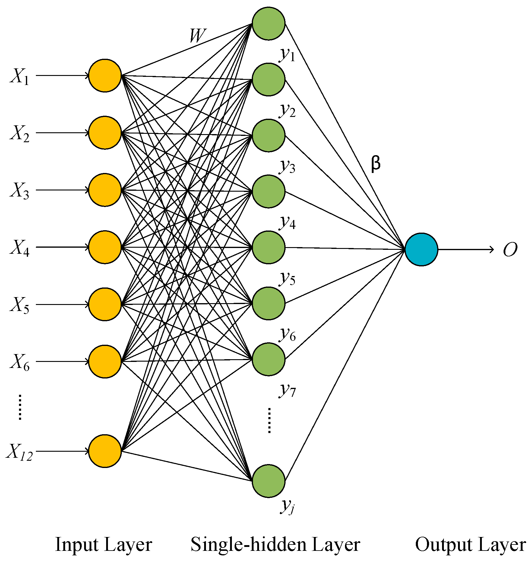
Gasoline blending is a continuous process without abrupt or substantial changes in blending events. Mathematically, parameters such as octane number during the gasoline blending process are continuous functions of the relevant blending parameters. An ELM model is employed to predict the octane number in gasoline blending. The ELM model uses a Single-Layer Feedforward Network (SLFN) with weights and biases randomly initialized, and the output layer weights are computed through a closed-form solution rather than iterative optimization. This method ensures high efficiency in the training process while maintaining high prediction accuracy. The key to establishing a neural network model involves determining the appropriate number of input and output parameters based on practical requirements, selecting a suitable network topology according to the characteristics of the study object, and deciding on the learning method and the number of neurons in the hidden layer based on the inherent patterns of the study object. Consequently, an initial analysis of the characteristics of the refinery’s gasoline production and blending units was conducted.
The primary gasoline blending components include fluid catalytic cracking gasoline, reformate gasoline (dearomatized), hydrocracked gasoline, hydrotreated gasoline, small amounts of additives such as methyl tert-butyl ether (MTBE), and alcohols. It is common to encounter an excess in octane numbers. Based on the demands of large-scale LP and operational experiences from multiple refineries of SINOPEC, it has been observed that certain parameters of specific gasoline blending components exhibit minor variations, such as the olefin, aromatic, and benzene contents in reformate gasoline, as well as the octane numbers of MTBE, xylene, MeOH, and EtOH components.
Considering these characteristics, this section identifies 12 input parameters that need to be included in the neural network model: the blending volumes of fluid catalytic cracking gasoline, reformate gasoline, hydrocracked naphtha, xylene, MTBE, MeOH, EtOH, and hydrotreated gasoline, as well as the octane numbers of fluid catalytic cracking gasoline, reformate gasoline, hydrocracked naphtha, and hydrotreated gasoline. Additionally, one output parameter, the octane number of the gasoline blend, is determined for the neural network model. These parameters are basic data that can be provided during the routine production process of the enterprise. Simultaneously, the neural network is tasked with predicting one output parameter: the octane number of gasoline. Given the practical nuances of gasoline blending in refineries, the neural network’s architecture will feature unipolar sigmoid functions for both forward and backward propagation across its input, hidden, and output layers. The topological structure of the gasoline blending ELM model is shown in Figure 2.
Specifically, due to the sensitivity of most refinery catalysts to elements such as sulfur, nitrogen, nickel, and vanadium in the feedstock, which can easily reduce reaction activity and catalyst lifespan, reasonable constraints are imposed on the feedstock streams of the unit [51]:
q f k , l q f k q f k , u
where q f k represents the property value k of feedstock f, and q s k , l and q s k , u , respectively, denote the upper and lower bounds constraints on this property. The product property constraints for gasoline, jet fuel, and diesel are based on the Chinese National Standards GB 17930-2016 [53], GB 6537-2018 [54], and GB 19147-2016 [55].

2.3. Carbon Footprint Tracking

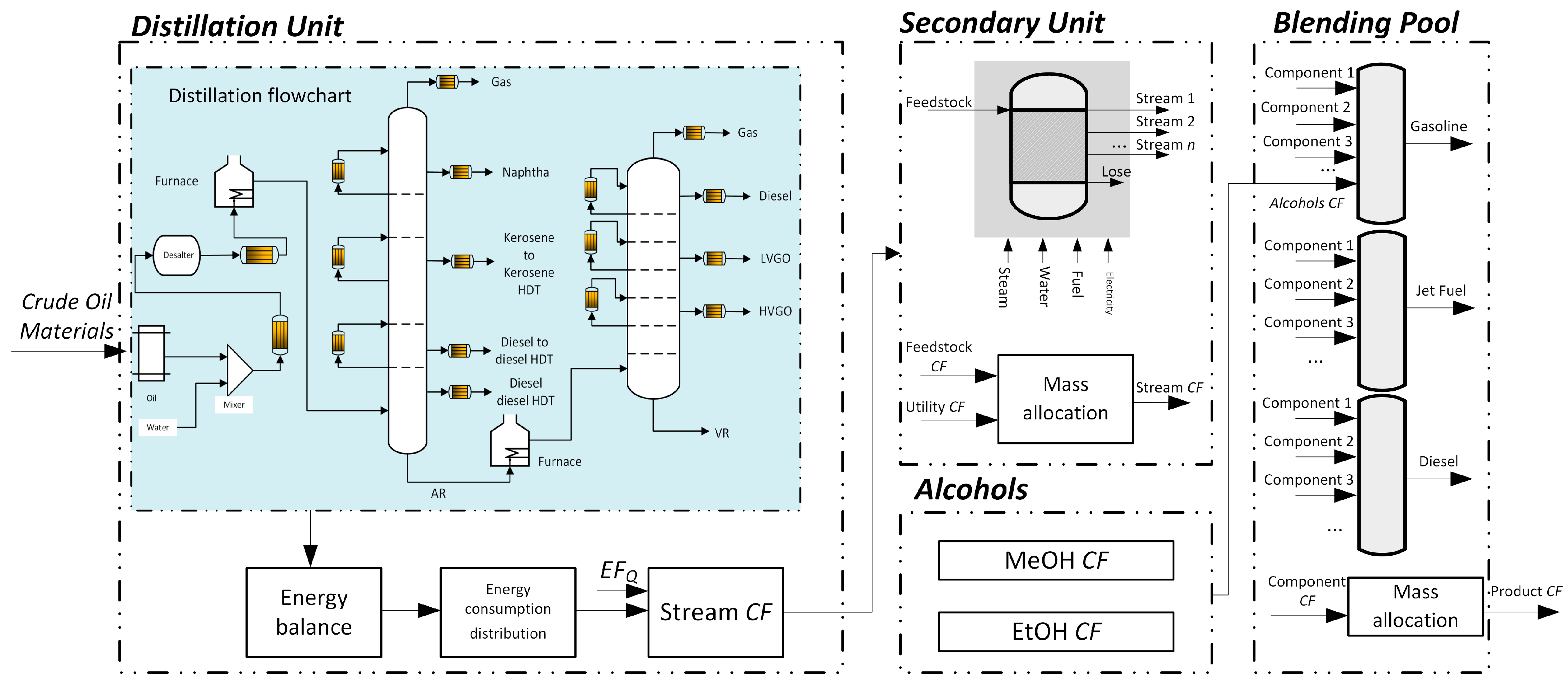
As illustrated in Figure 3, This study focuses on assessing the gasoline carbon footprint within the refinery scope and establishes a unified evaluation framework that encompasses the carbon footprint generated, transferred, and blended throughout the processes of crude oil intake, distillation, secondary processing, and product blending. The evaluation framework does not consider the carbon emissions produced during the combustion of gasoline.
The carbon footprint of distillation unit side streams is computed using energy consumption allocation. Based on crude oil processing volume and the process design and parameter calculations of primary processing units, the steam and fuel consumed and produced by each distillation unit side stream are determined. This energy consumption is then converted into corresponding carbon footprints. The model utilizes a three-column distillation process, with both atmospheric and vacuum towers incorporating three stages of stripping. Side products undergo heat recovery to recover thermal energy. By accounting for feed heat exchange energy, heating energy, heat release within the fractionation column, and internal heat exchange energy within the unit, a calculation model for the carbon footprint of individual side streams is established [51]. The detailed calculation model is outlined in Section S1 of the Supplementary Information.
The carbon footprint of side streams from secondary processing units is determined using a mass allocation approach. Initially, this involves accounting for the carbon footprint carried by the feedstock and the footprint generated by the unit’s utility consumption. Subsequently, the carbon footprint is distributed based on the mass proportions of the side-stream logistics, accounting for losses and waste carbon footprints attributed to intermediate materials and products. This allocation process is formulated as shown in Formula (5) [51]:
C F o u t = A × C F i n + B
where A and B are transfer coefficients between the carbon footprint of the feedstock, CFin (kgCO2/t), and the carbon footprint of the product, CFout (kgCO2/t). A is assigned based on the unit properties, typically set to 1 under normal circumstances. B represents the carbon emissions from utilities and processes, calculated using Formula (6) [51]:
B = i C F u , i + j C F f , j
where CFu,i (kgCO2/t) denotes the carbon emission intensity of the i-th utility materials, and CFf,j represents the carbon emission intensity of the j-th process, typically attributed to emissions from catalyst coke burning. The utilities consumed by each unit and CFu,i values are detailed in Tables S2 and S3, respectively. In cases of multiple stream convergence, the carbon footprint is treated as a physical property and undergoes linear blending.
Moreover, integrating the carbon footprint tracking model with the global LP model enables comprehensive carbon balance accounting across the entire plant. This approach tracks the carbon footprint of intermediate materials and traces the carbon footprint of final products, ensuring thorough carbon footprint management and reporting.

2.4. LP-ELM Framework

Integrating the LP and ELM models significantly affects the solution speed of the global planning model, making it challenging to solve directly with standard solvers. This section proposes an LP-ELM integration framework to address these challenges. The framework involves the following steps: First, data is collected, preprocessed, and used to train the ELM model. The octane number is treated as a linear blending property, and the blended gasoline octane number is predicted using Formula (3). The LP model is then solved using the SciPy library to obtain the optimal blending component quantities. Next, the obtained blending component quantities are input into the ELM model to predict the octane number and verify its compliance with the constraint conditions. If the predicted octane number is below the required constraint, the lower bound constraint on the octane number in the LP model is increased. Conversely, if the predicted octane number exceeds the requirement, the lower bound constraint in the LP model is decreased. Through iterative adjustments, this process yields a blending scheme that accurately describes the gasoline octane number, along with the product’s carbon footprint, gross margin (GM), and global mass flow balance. The proposed LP-ELM framework solution process is illustrated in the following pseudocode (Algorithm 1).
Algorithm 1 Integration of LP and ELM for Octane Blending Optimization
Input: LP input (raw material constraints, device capacity, yield of device side line, stream properties, property constraints, product constraints, utility consumption, price system), ELM input (blending component octane number data)
Output: Blending scheme, carbon footprint of products, GM, global flow balance
1. Start
2. Collect data and preprocess data
3. Build and train ELM neural network model
4. Build LP model
5. Define objective function: Maximize gross margin
6. Set initial optimization parameters
7. while not Convergence do
8.      Solve LP model by SciPy
9.      Obtain optimal blending solution: Blending component quantities
10.    ELMPredictRON ELM_predict(BlendingComponentQuantities)
11.    if ELMPredictRON > OctaneConstrainLowerBound then
12.        RONLowerBound(LP model) = RONLowerBound(LP model) + δ
13.    else if ELMPredictRON > RONConstrainLowerBound then
14.      RONLowerBound(LP model) = RONLowerBound(LP model) − δ
15.    end if
16.    if TerminationConditionMet then
17.       Output results
18.      break
19.    end if
20. end while
21. Output final optimization solution
22. end

2.5. Alcohol-Based Blendstock Break-Even Value Characterization

The break-even value (BEV) for an alcohol-based blendstock, or any other refinery input, is defined as the maximum calculated purchasing cost that maintains an equivalent GM under the same conditions without the purchase. This valuation method is consistent with industry practices for decisions such as crude oil acquisitions and alcohol-based blendstock research [43].
B E V = G M a l c o h o l s G M b a s e m a l c o h o l s
In this study, the calculation of bioEtOH BEV proceeds through the following steps: First, model inputs are fixed, including the Saudi Medium crude oil price, refinery configuration, alcohol blendstock candidates, and blending levels. Next, the refinery model is optimized using the proposed LP-ELM framework to establish the baseline gross margin (GMbase) without purchasing alcohol blendstocks. Subsequently, the model is re-optimized with alcohol blendstock prices set to zero, yielding the gross margin (GMalcohols). The BEV is then computed by dividing the profit difference obtained from these optimizations by the mass of purchased alcohol blendstocks (malcohols), as detailed in Formula (7).

2.6. Price System Establishment

Crude oil procurement constitutes the most substantial expense in the refining industry. The properties of crude oil, such as its API gravity, sulfur content, total acid number (TAN), and formula, dictate its processing complexity and the yield of high-value products, thereby influencing its market price. Using the average price of West Texas Intermediate (WTI) crude oil from April 2020 to March 2023, sourced from the U.S. Energy Information Administration (EIA) [56], as a benchmark, the price of crude oil is determined based on these specified parameters [43,57]. Based on historical WTI prices and product price data [58], linear regression was performed to calculate the corresponding product prices. The detailed fitting process and price data are provided in Figure S1.

2.7. Case Studies

Within the same refinery framework, this study evaluates the economic and environmental performance of alcohol–gasoline blends derived from various technological pathways. It considers three types of MeOH and three types of EtOH as potential gasoline blending alcohols, namely, coal-based MeOH (CtM), biomass-based MeOH (BioM), MeOH from carbon capture and usage (CCUM), coal-based EtOH (CtE), EtOH from corn (CornE), and EtOH from straw (StrawE). Furthermore, to assess the economic viability of alcohol-blended gasoline, future trends in carbon taxes are incorporated. Consequently, the study designs cases encompassing all these factors, analyzing GM, BEV, product carbon footprint, and carbon emissions. The plant scenarios are tailored for construction in mainland China, with unspecified costs estimated reasonably based on local market prices. Detailed costs of raw materials and product prices utilized in the analysis are outlined in Table 2. Saudi Medium Crude Oil is utilized as a feedstock for processing. The data employed in this paper are grounded on a rational assumption presented in the referenced literature [22,32,59,60,61,62,63]. In this study, an integrated refinery with an annual processing capacity of 12 million tons was selected as the baseline case. The lower and upper bounds for gasoline yield in the evaluated processing routes are set at 90% and 110% of the gasoline yield in the baseline case, respectively. The refinery is equipped with hydrogenation and decarbonization units, the capacities of which are detailed in Table S4.

3. Results and Discussion

3.1. RON Prediction

3.1.1. Parameter Settings

Prior to simulation, the parameter settings play a crucial role in the predictive performance of the neural network. To optimize model parameters, the dataset is divided into 70% for the training set, 15% for the validation set, and 15% for the test set. Initially, the model is developed using 60% of the training set, and then the model parameters are adjusted using 20% of the validation set [64]. Once the optimal parameters are determined, the combined training and validation sets are used to train the final model. The test set is subsequently used to evaluate the model’s performance. In this study, the regularization parameter for the ELM model is set to 0.001, and the learning rate is set to 0.001.

3.1.2. RON Prediction Results

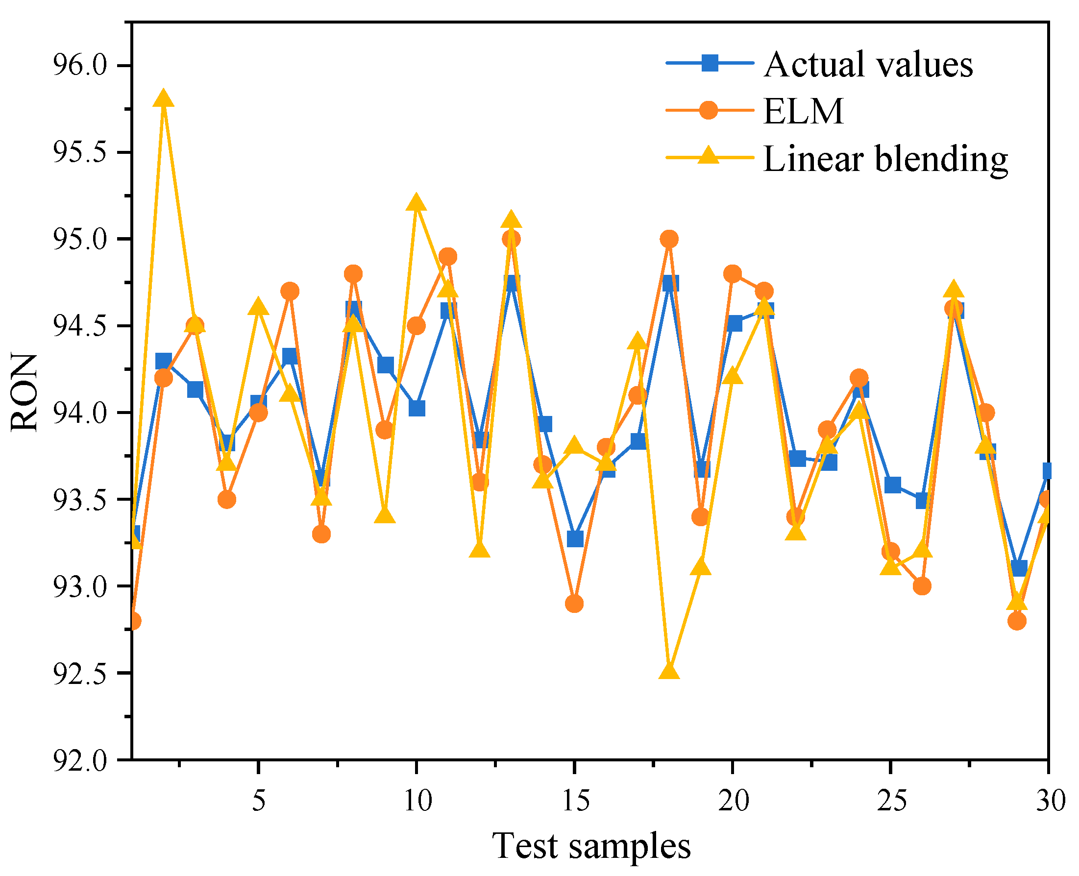
A dataset comprising 200 production records from a real-world refinery was utilized as the raw data to train the developed ELM model. The trained model’s prediction accuracy was validated using a test set. Simultaneously, the linear blending model, which is the current mainstream method, was also employed for predicting the RON of gasoline blends for comparison with the ELM model. In the evaluation of machine learning models, the choice of appropriate error metrics is pivotal for accurately assessing predictive performance. The Mean Absolute Error (MAE), functioning as an unbiased estimator, effectively captures the average magnitude of discrepancies between predicted and observed values, particularly adept in contexts involving outliers or noisy data. Meanwhile, the Mean Squared Error (MSE) and Root Mean Squared Error (RMSE) prioritize squared errors, imposing heightened penalties on larger deviations, thereby suitable for rigorously evaluating model accuracy [50]. The Coefficient of Determination (R2), quantifying the proportion of variance in the target variable explained by predicted values, provides a robust measure for assessing model fit and generalization capabilities. The comprehensive application of these error metrics facilitates a thorough evaluation of predictive performance and practical applicability in real-world scenarios.
As illustrated in Figure 4, the predictions generated by the ELM align more closely with the actual RON compared to those from the linear blending model, and they do not exhibit significant outliers. This observation is further substantiated by the error analysis results presented in Table 3. The ELM model demonstrates lower MAE, MSE, and RMSE relative to the linear blending model, indicating superior accuracy in capturing the true data variations and greater robustness against large deviations. Furthermore, the ELM model’s coefficient of determination (R2) approaches 1, signifying a higher explanatory power for data variability and a more accurate fit between predicted and actual values. Consequently, the ELM model exhibits a notable advantage over the traditional linear blending model in the prediction of octane numbers. Due to the multitude and complexity of factors affecting gasoline RON, existing machine-learning models exhibit certain degrees of error. The objective of this study is to develop an ELM model for the rapid prediction of gasoline blending octane values. However, to achieve more precise predictive performance, extensive additional work is required.

3.2. Economic Performance Comparison

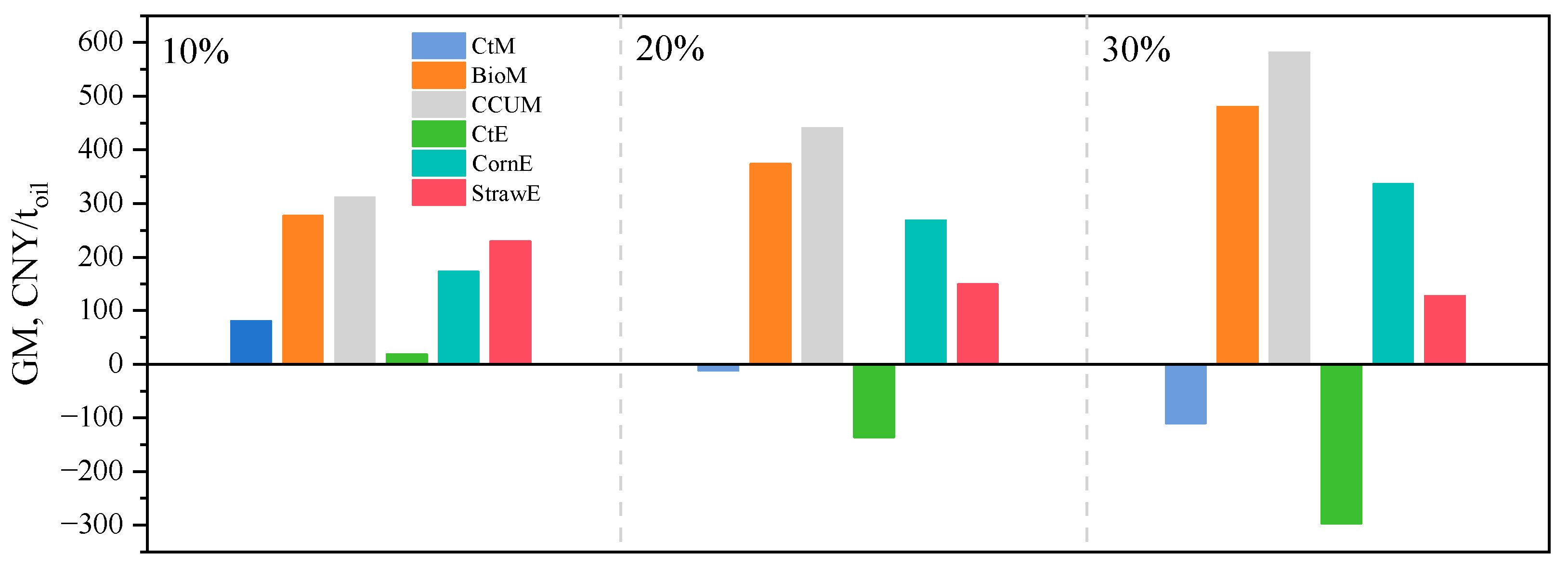
In this study, the economic performance of six types of alcohols blended into gasoline at different blending ratios was analyzed in relation to refinery operations. Many countries and regions have regulations specifying certain blending ratios for biofuels. For example, China’s ‘Regulations on the Management of EtOH Gasoline’ stipulates a 10% EtOH blending ratio. In the research and experimental phases, varying blending ratios may be employed to assess their impact on performance, emissions, and economic viability. Excessively high blending ratios can adversely affect engine performance and durability. Based on existing studies, the blending ratios selected in this paper are 10%, 20%, and 30% [13,43]. The lower and upper bounds for gasoline yield in the evaluated processing routes are set at 90% and 110% of the gasoline yield in the baseline case, respectively. The overall GM was calculated and compared with the base case where no alcohols were blended, as shown in Figure 5.
The results indicate that blending CtM, BioM, and CtE can enhance the economic benefits of refineries compared to the base case. CtM demonstrates the most significant economic advantage, particularly at a 30% blending ratio, achieving a GM of 778.12 CNY/toil, significantly higher than the base case. Biomass-based BioM also benefits from lower production costs, enhancing refinery profitability with a GM of 596.91 CNY/toil at a 30% blending ratio, second only to CtM. However, the economic performance of refineries adopting CCUM is markedly lower due to the high costs associated with hydrogen electrolysis for raw material production. At a 30% blending ratio, the refinery’s GM with CCUM is 8.91 CNY/toil, only 1.88% of the base case. EtOH derived from coal and biomass generally performs less favorably compared to MeOH, thus refineries blending EtOH into gasoline may not achieve the same economic performance as those using MeOH. This is attributed to the production characteristics of MeOH, which can be synthesized directly from coal-derived synthesis gas, whereas EtOH’s production pathway is longer and costlier in most scenarios. Refineries utilizing first-generation and second-generation biomass MeOH show slightly reduced GM compared to the base case. Currently, adopting low-cost MeOH appears to be a highly beneficial direction for refineries seeking to enhance gasoline yields. Despite being a promising emerging pathway, the high costs associated with CCUM remain a significant barrier to its widespread adoption.

3.3. Carbon Footprint

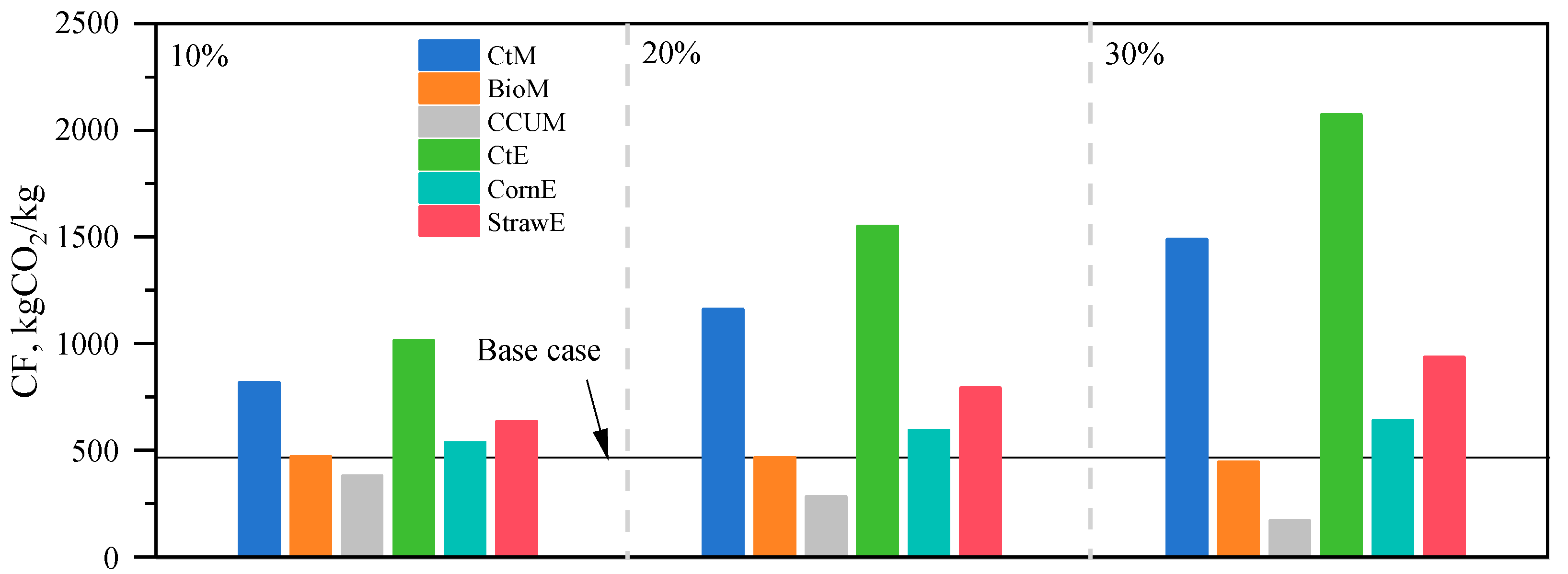
Based on the LP-ELM framework, the gasoline blending schemes and the overall plant carbon footprint transfer model for all technical routes were calculated, and the carbon footprints of gasoline are shown in Figure 6. A very notable feature is that the CtM and CtE processes, which originate from coal, have the highest gasoline carbon footprints. Specifically, the CtE process reaches the highest carbon footprint of 2072.89 kgCO2/kg at a 30% blending ratio. Although these two processes exhibit significant economic competitiveness, they also result in the most severe carbon emissions. This is primarily due to the mismatch between the hydrogen and carbon ratios in coal-based alcohols, which necessitates the consumption of CO through the water-gas shift unit to supplement hydrogen. This results in carbon wastage and emissions. The CtE production process, which predominantly uses an indirect method in the market, involves coal gasification to syngas, followed by MeOH synthesis, carbonylation to acetic acid, and subsequent hydrogenation to EtOH. The extended reaction pathway leads to a higher CF. Biomass MeOH has a slightly lower CF compared to the base case, while first-generation and second-generation bioEtOH have CFs slightly higher than the base case. The differences in raw material costs and technology maturity result in the second-generation bioEtOH technology currently being slightly inferior to the first-generation bioEtOH technology in both economic and environmental performance.
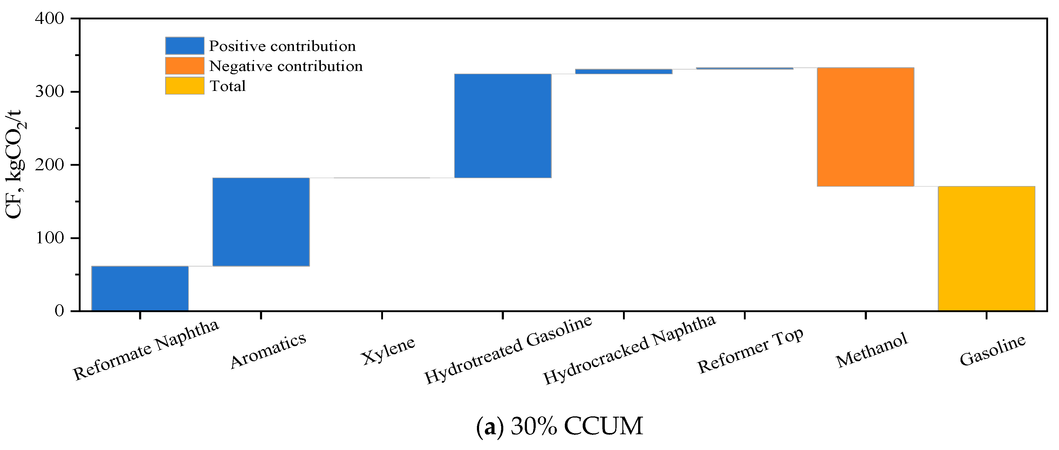
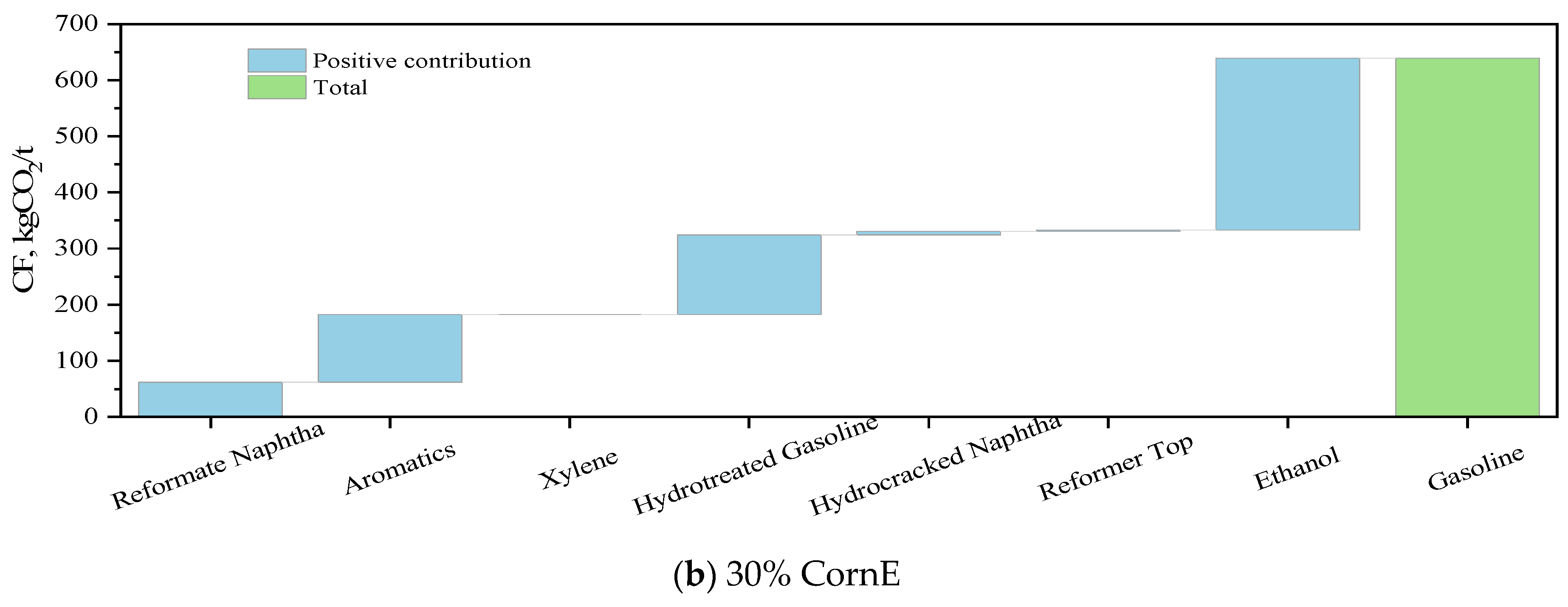
Furthermore, the gasoline CF can be analyzed based on the blending schemes and the CF data of the blending components. The gasoline CF blending data for two typical technical routes, CCUM and CornE, are presented in Figure 7. As shown in Figure 7a, seven components are used for gasoline blending: naphtha and raffinate from the catalytic reforming unit, aromatics, xylene, hydrotreated gasoline, hydrocracked naphtha, and MeOH. The figure illustrates the contribution of each component to the CF. The major contributions originate from the reforming unit, aromatics, and the hydrotreating unit. The reforming unit components contribute significantly to the CF due to their large volume, while the hydrotreating products have a high carbon intensity because of the extensive processing routes involved (starting from distillation and potentially passing through delayed coking, residue hydrotreating, catalytic cracking, and hydrotreating), which leads to a higher CF in the final product. CCUM, due to its ability to consume CO2 during production, possesses a negative carbon emission attribute, significantly reducing the gasoline CF when blended. Therefore, when blending alcohols to reduce the CF, maximizing the blending ratio is a favorable strategy. As illustrated in Figure 7b, CornE, which is considered to have the lowest CF among EtOHs, still contributes more than 47.9% to the gasoline CF when blended. This indicates that the high CF characteristic of EtOH makes its blending process non-conducive to carbon reduction and may instead increase environmental costs.

3.4. Future Trend Analysis

3.4.1. Cost Trend of Alcohols

Currently, biomass MeOH and biomass EtOH do not dominate the market, especially in China, where their technological maturity is increasing and installed capacity is also on the rise [65]. Compared to the widely commercialized coal-based processes, biomass alcohols and CCUM have significant potential for cost reduction. The promotion of small-scale distributed biomass-based alcohol technologies is expected to significantly reduce the transportation costs of methanol and ethanol [66]. For CCUM, several studies indicate that renewable energy generation is expected to achieve remarkable development and cost reductions over the next decade. Utilizing renewable energy for hydrogen production, which is then used to produce MeOH, represents a route with substantial economic potential. Several studies [67] have reported on the future cost predictions for biomass alcohols and renewable energy. However, these results have not been presented within a unified framework, making it difficult to perform a cross-comparison of the alcohols mentioned in this study. Therefore, this study attempts to predict the price variations of alcohols using a damped exponential growth model [68], formulated as follows:
C t = a · e r t + b
where Ct represents the price at time t and the parameters a, b, and r denote the initial value, the asymptotic value, and the growth rate, respectively. Based on the alcohol costs provided in the literature for 2020 and the estimated costs for 2030, this model was used to estimate the costs of biomass alcohols from 2020 to 2050. The parameters for the cost estimation models of each type of EtOH are presented in Table S5.
According to the proposed cost prediction model, the prices of biomass alcohols and CCUM were forecasted, and the results are shown in Figure 8. The future carbon tax trend in mainland China, as provided in the literature [51,69], was adopted for the long-term performance evaluation of the refinery. As illustrated in Figure 8, the costs of biomass MeOH and EtOH decrease with technological advancements and market expansion, particularly before 2035. Second-generation bioEtOH is expected to become cheaper than first-generation bioEtOH by around 2030. The production of StrawE avoids the resource waste associated with using food crops as raw materials by utilizing straw instead. This indicates that StrawE will surpass first-generation biomass MeOH comprehensively after 2030. The price reduction trend of CCUM is the most significant among all alcohols. Benefiting from the rapid decline in renewable electricity costs, CCUM is projected to become cheaper than bioEtOH by around 2030 and further decrease to 1887.6 CNY/t by 2050, making it the most cost-effective alcohol production route. The CtM and CtE processes are assumed to have constant costs. As other renewable energy routes develop, these processes will gradually lose their price advantage.

3.4.2. Estimating the Break-Even Value

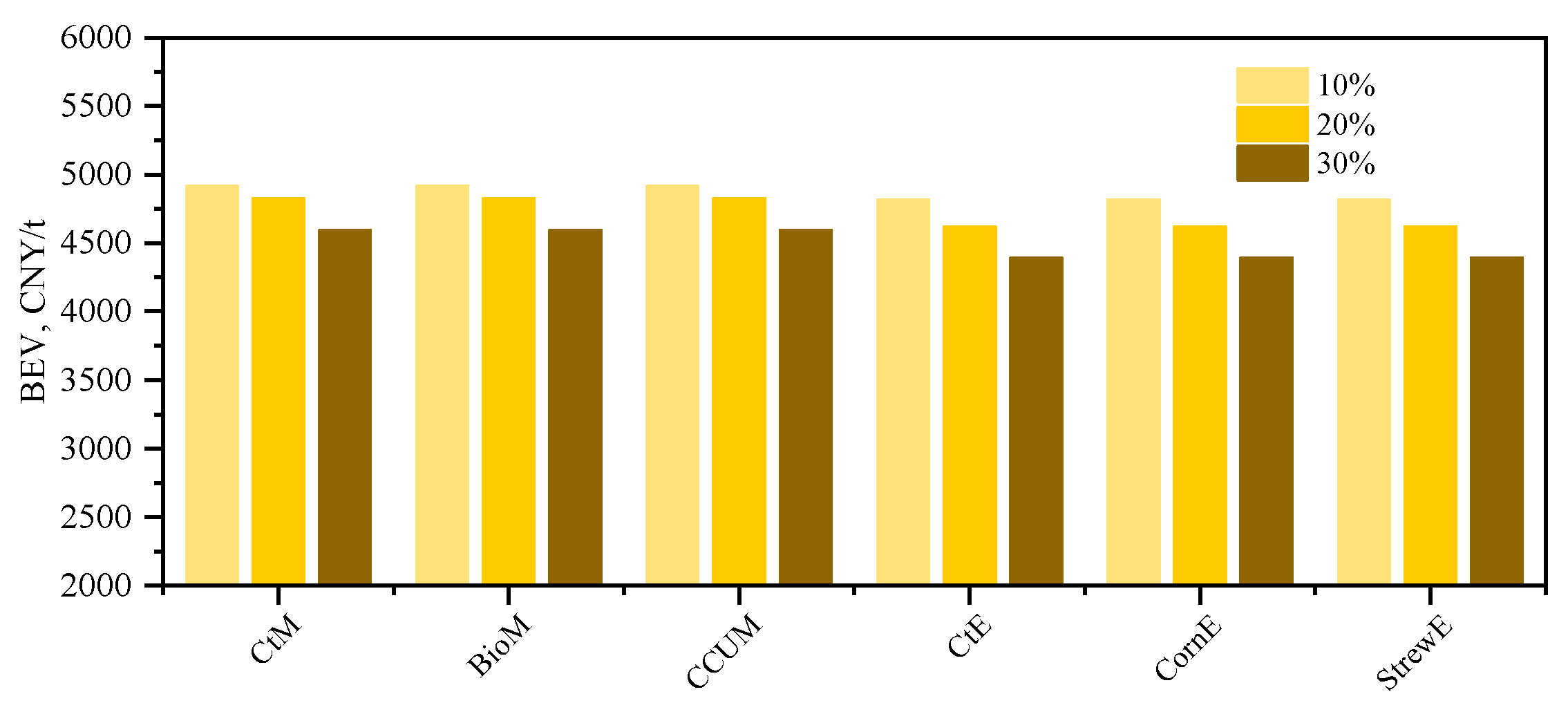
Figure 9 presents the BEV values of case refineries at different alcohol blending levels under current scenarios. According to the BEV calculation formula (Formula (7)), the calculation process is independent of alcohol prices. BEV serves as an indicator for evaluating the economic performance contribution of alcohols; the higher the BEV, the easier it is for refineries to increase profitability. MeOH has a RON of 155, while EtOH has a RON of 111. Consequently, blending MeOH results in less pressure on gasoline blending specifications, making it easier for refineries to profit. As shown in Figure 9, the BEV of refineries blending MeOH is slightly higher than those blending EtOH, supporting this observation.
Under the projected future scenario of decreasing alcohol costs and increasing carbon taxes, the BEVs for refineries have been calculated and are shown in Figure 10. Overall, as time progresses, the BEVs for CtM, CtE, CornE, and StrawE exhibit a declining trend. This suggests that the high carbon intensity of these processes results in additional costs, making the cost requirements for raw materials more stringent. The BEV for BioM remains relatively stable because its carbon intensity is similar to that of gasoline, rendering it less susceptible to carbon taxes. Notably, the BEV for CCUM demonstrates an increasing trend in the future, indicating that blending CCUM is expected to become more profitable. Furthermore, this economic advantage is projected to expand over time.
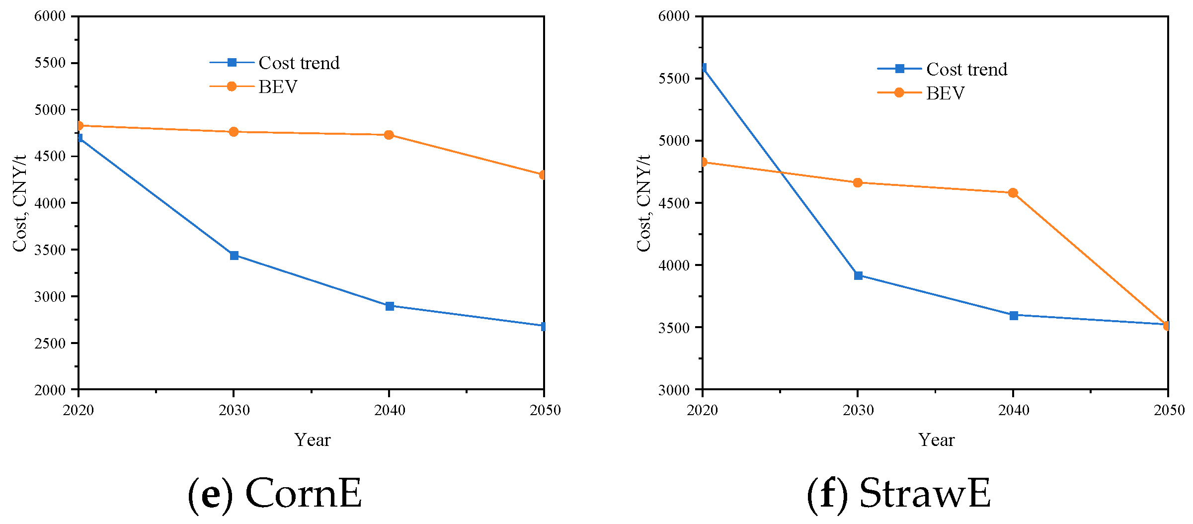
To explore the future economic performance of different alcohols, we compared the trends of alcohol costs with BEV trends, as illustrated in Figure 11. For CtM (Figure 11a), costs remain below its BEV for most of the projected period. This indicates that CtM benefits from established production processes and scale, maintaining low costs. This low-cost advantage enables refineries to absorb the additional costs associated with increased carbon emissions when blending CtM. However, around 2050, CtM is projected to incur negative returns for refineries due to high carbon taxes. Conversely, CtE, another coal-based product, is expected to see its BEV drop below EtOH costs around 2040, losing its low-cost advantage even earlier. BioM and CornE, benefiting from declining costs, are expected to positively impact refinery profits from 2020 to 2050. StrawE is projected to contribute positively to refinery profits from 2025 to 2050, but it may lose this advantage beyond 2050. CCUM is anticipated to start positively impacting refinery profits around 2027 and to continue expanding this advantage into the future, emerging as the most economically promising process.
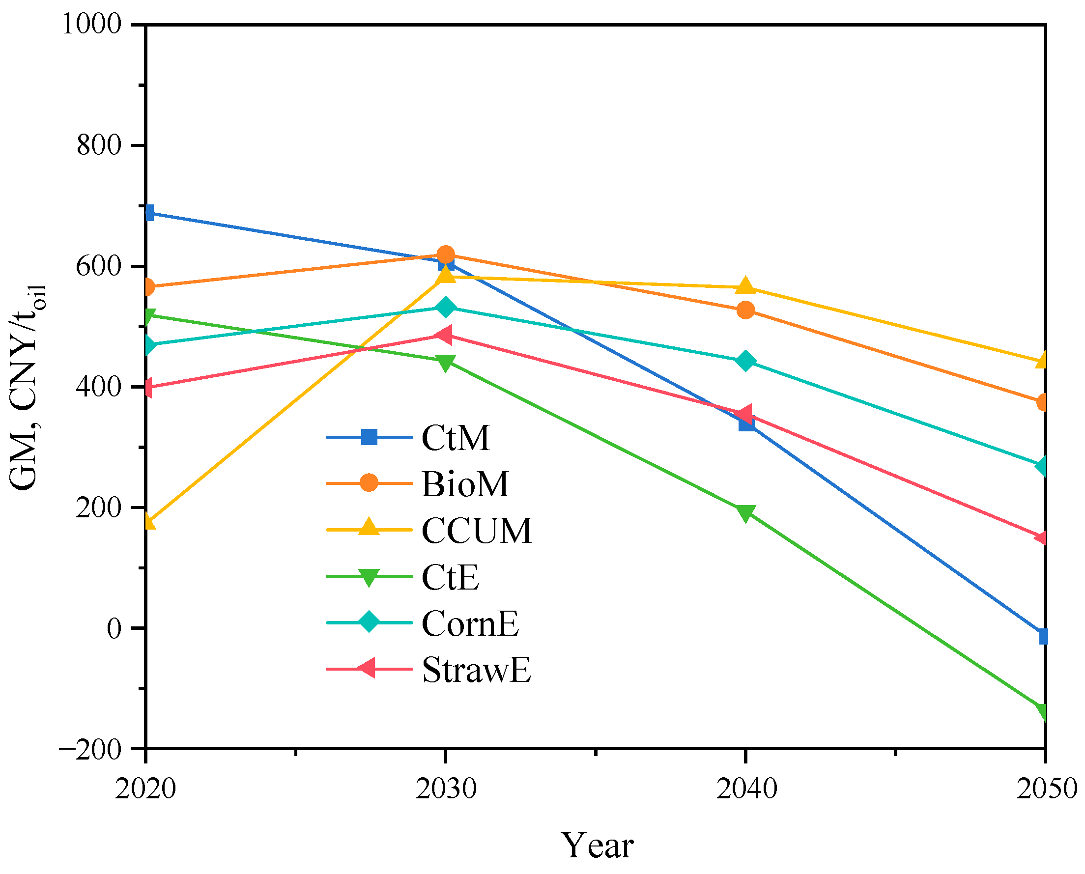
Figure 12, based on GM analysis, further substantiates the aforementioned conclusions. Under projected high carbon taxes, coal-based alcohols are forecasted to lose economic competitiveness, ranking lowest among all considered types. By approximately 2035, CCUM emerges as the optimal choice for gasoline blending due to its superior economic and environmental performance, with this advantage expected to expand over time. Biomass-based MeOH demonstrates economic advantages over biomass-based EtOH, suggesting that biomass-to-MeOH production is a preferable option for fuel production, provided engine compatibility allows. Before 2030, the decline in the costs of CCUM, biomass MeOH, and biomass EtOH enhances the profitability of refineries, surpassing those blended with CtE by 2030. This indicates a rapid advancement period for related technologies and facility capacities from now until 2030. Notably, the GM of refineries blending CCUM increases by 236% compared to 2020, approaching the level of CtM. Overall, the anticipated rapid increase in carbon taxes results in varying declines in GM for all studied refineries after 2030. This highlights the necessity for refineries to adopt comprehensive carbon reduction strategies to sustain profitability.
Figure 13 and Figure 14 illustrate refinery GM and gasoline CF for the 2050 operating year at various blending levels. The analysis indicates that increasing the blend percentage of CCUM significantly enhances refinery GM and reduces the gasoline CF, whereas other alcohol production pathways impose greater carbon mitigation pressures on refineries. Refineries achieving a 30% CCUM blend attain a GM of 581.75 CNY/toil, exceeding the baseline by 32%. Conversely, refineries blending higher ratios of coal-based MeOH and EtOH show negative economic impacts, suggesting that fossil-energy-based alcohols are unlikely to be considered for gasoline blending in 2050. As profit-oriented enterprises, refineries prioritize maximizing efficiency. Some perspectives suggest that blending alcohols into gasoline is perceived as a strategy to reduce gasoline’s CF. However, detailed analysis reveals that bio-MeOH and bio-EtOH, although often promoted as renewable fuels, do not positively contribute to carbon emission reductions. Instead, bio-EtOH imposes cost pressures on refineries.

3.5. Outlook

Current research predominantly focuses on the environmental advantages of alcohol-blended gasoline in spark-ignition engines [11,39,41]. These benefits include better combustion efficiency, lower CO emissions, and reduced acidic gas emissions [16,18,36]. However, there are also some drawbacks: lower calorific value, production of acidic by-products during combustion, and a tendency for phase separation [12,70]. With advancements in related technologies, new engine designs have increased tolerance for these drawbacks. Specifically, alcohols derived from biomass are considered sustainable and low-carbon, making them widely regarded as excellent components for gasoline blending [40,71].
However, through the unified refinery-wide assessment framework established in this study, blending alcohols into gasoline has not realized the expected advantages over traditional gasoline production processes. Most biomass-derived alcohols exhibit higher carbon intensity in their production processes compared to traditional gasoline, thereby increasing the gasoline’s CF post-blending. Moreover, these alcohols face significant challenges such as lower technological maturity and limited equipment capacities compared to coal-based processes, rendering their production costs economically uncompetitive. This compromises both the economic viability and environmental performance of refineries when incorporating biomass-derived alcohols. Looking ahead, with anticipated rises in carbon emission costs, these challenges are likely to intensify. However, there is optimism regarding carbon-dioxide-hydrogenation-produced MeOH (CCUM), which is currently garnering significant attention. Despite higher current costs, CCUM offers negative carbon emissions, making it well-positioned to excel in future scenarios with high carbon costs. Ongoing research efforts are actively refining catalysts and production processes, aiming for continuous improvements. This positions CCUM-blended gasoline to potentially achieve substantial economic and environmental advantages beyond 2030. In recent years, China has been vigorously promoting the blending of MeOH and EtOH in gasoline [72,73]. However, the additional carbon burden after blending alcohols should be a matter of serious consideration. The sources and optimal selection of alcohols will also be focal points of concern for the government, researchers, and businesses.

4. Conclusions

This study aims to enhance refinery sustainability through alcohol-based gasoline blends and explore the market potential for new alcohol types. The key conclusions are as follows:
ELM Model Performance: ELM accurately predicts the octane rating of alcohol-blended gasoline, outperforming traditional models. The LP-ELM framework allows comprehensive refinery GM estimations and CF tracking.
Economic and Environmental Impact: Coal-based MeOH currently offers the best economic performance at a 30% blending ratio, achieving a GM of 778.12 CNY/toil but with the highest gasoline CF of 2072.89 kgCO2/t. Conversely, CCUM blending yields the poorest economic performance with a GM of 8.91 CNY/toil, representing only 1.88% of the base case without alcohol blending, but it significantly reduces gasoline CF by 62.4%.
Impact of Rising Carbon Taxes: Rising carbon taxes will erode the economic advantages of CtM and coal-based EtOH (CtE). By 2050, a 20% CtM blend will have negative economic contributions, and CtE will follow by 2040.
Future of Biomass Alcohols: Biomass alcohols are expected to maintain positive economic contributions due to cost reductions from technological maturity. However, second-generation biomass EtOH may not outperform first-generation EtOH economically.
Future of CCUM: Despite higher current costs, CCUM’s negative carbon emissions will become increasingly advantageous in future high carbon emission cost scenarios. Research in catalyst development and production processes is optimizing CCUM, making it poised to achieve significant economic and environmental benefits after 2030.
Overall Recommendations: CCUM is the preferred blending material for future refineries. For biomass alcohols, technological advancements and cost reductions are critical. Coal-based MeOH and EtOH are likely to be phased out due to their high carbon emissions. Given stricter carbon emission policies, these projections may materialize sooner than expected.

Supplementary Materials

The following supporting information can be downloaded at: https://www.mdpi.com/article/10.3390/pr12081751/s1, Figure S1. Product price fitting; Table S1. Side streams yields; Table S2. Utilities consumption; Table S3. Material carbon footprint; Table S4. Design parameters of base case process; Table S5. The parameters for the cost estimation models.

Author Contributions

Conceptualization, X.S. and B.C.; methodology, X.S.; software, B.C. and Y.F.; validation, T.L. and Z.Y.; formal analysis, X.S. and S.W.; investigation, X.S.; resources, Z.Y. and B.C.; data curation, B.C.; writing, X.S. and B.C. All authors have read and agreed to the published version of the manuscript.

Funding

This research was funded by the National Key Research and Development Program of China, grant number 2022YFB3305905.

Data Availability Statement

Data are contained within the article.

Conflicts of Interest

Authors Xiaofei Shi, Zihao Yu, Tangmao Lin, Sikan Wu, Yujiang Fu and Bo Chen were employed by the company SINOPEC Dalian Research Institute of Petroleum and Petrochemicals Co., Ltd. The remaining authors declare that the research was conducted in the absence of any commercial or financial relationships that could be construed as a potential conflict of interest.

Nomenclature

AIArtificial intelligence
ANNsArtificial neural networks
BioMBioMeOH
CBFECoal-based fuel EtOH
CCUMMeOH from carbon capture and usage
CFCarbon footprint
CornECorn to EtOH
CtECoal-based EtOH
CtMCoal-based MeOH
E1515% EtOH
EIAEnergy information administration
ELMExtreme Learning Machine
FGFBFirst-generation fuel bioEtOH
GAGenetic algorithms
GCMGroup contribution method
GMGross margin
LP-ELMA model framework integrating LP model and ELM model
M1515% MeOH
MAEMean absolute error
MeOHMeOH
MONMotor octane number
MSEMean squared error
MTBEMethyl tert-butyl ether
R2Coefficient of determination
RFRandom forest
RMSERoot mean squared error
RONResearch octane number
SGFBSecond-generation fuel bioEtOH
SLFNSingle-layer feedforward network
StrawEStraw to EtOH
TANTotal acid number
WTIWest Texas intermediate

References

  1. Kloth, M. Transport Demand Set to Triple, But Sector Faces Potential Disruptions. Available online: https://www.itf-oecd.org/transport-demand-set-triple-sector-faces-potential-disruptions (accessed on 2 July 2024).
  2. Liu, J.; Li, S.; Ji, Q. Regional differences and driving factors analysis of carbon emission intensity from transport sector in China. Energy 2021, 224, 120178. [Google Scholar] [CrossRef]
  3. Agency, I.E. Global EV Outlook 2024; International Energy Agency: Paris, France, 2024. [Google Scholar]
  4. Oh, J.J. The 500-Million-Vehicle Question: What Will It Take for China to Decarbonize Transport? Available online: https://blogs.worldbank.org/en/transport/500-million-vehicle-question-what-will-it-take-china-decarbonize-transport#_ftn1 (accessed on 2 July 2024).
  5. Yu, X.; Sandhu, N.S.; Yang, Z.; Zheng, M. Suitability of energy sources for automotive application–A review. Appl. Energy 2020, 271, 115169. [Google Scholar] [CrossRef]
  6. Liu, Y.; Cruz-Morales, P.; Zargar, A.; Belcher, M.S.; Pang, B.; Englund, E.; Dan, Q.; Yin, K.; Keasling, J.D. Biofuels for a sustainable future. Cell 2021, 184, 1636–1647. [Google Scholar] [CrossRef]
  7. Kenkel, P.; Wassermann, T.; Zondervan, E. Renewable Fuels from Integrated Power- and Biomass-to-X Processes: A Superstructure Optimization Study. Processes 2022, 10, 1298. [Google Scholar] [CrossRef]
  8. Montoya Sánchez, N.; Link, F.; Chauhan, G.; Halmenschlager, C.; El-Sayed, H.E.; Sehdev, R.; Lehoux, R.; de Klerk, A. Conversion of waste to sustainable aviation fuel via Fischer–Tropsch synthesis: Front-end design decisions. Energy Sci. Eng. 2022, 10, 1763–1789. [Google Scholar] [CrossRef]
  9. Ampah, J.D.; Liu, X.; Sun, X.; Pan, X.; Xu, L.; Jin, C.; Sun, T.; Geng, Z.; Afrane, S.; Liu, H. Study on characteristics of marine heavy fuel oil and low carbon alcohol blended fuels at different temperatures. Fuel 2022, 310, 122307. [Google Scholar] [CrossRef]
  10. Li, C.; Negnevitsky, M.; Wang, X. Prospective assessment of methanol vehicles in China using FANP-SWOT analysis. Transp. Policy 2020, 96, 60–75. [Google Scholar] [CrossRef]
  11. Iliev, S. A Comparison of Ethanol, Methanol, and Butanol Blending with Gasoline and Its Effect on Engine Performance and Emissions Using Engine Simulation. Processes 2021, 9, 1322. [Google Scholar] [CrossRef]
  12. Liu, W.; Shadloo, M.S.; Tlili, I.; Maleki, A.; Bach, Q.-V. The effect of alcohol–gasoline fuel blends on the engines’ performances and emissions. Fuel 2020, 276, 117977. [Google Scholar] [CrossRef]
  13. Fan, Q.; Liu, S.; Qi, Y.; Cai, K.; Wang, Z. Investigation into ethanol effects on combustion and particle number emissions in a spark-ignition to compression-ignition (SICI) engine. Energy 2021, 233, 121170. [Google Scholar] [CrossRef]
  14. Likhanov, V.; Lopatin, O. Study of toxicity of diesel engine on alcohol fuel. IOP Conf. Ser. Earth Environ. Sci. 2020, 421, 072018. [Google Scholar] [CrossRef]
  15. Çelebi, Y.; Aydın, H. An overview on the light alcohol fuels in diesel engines. Fuel 2019, 236, 890–911. [Google Scholar] [CrossRef]
  16. Balki, M.K.; Sayin, C.; Canakci, M. The effect of different alcohol fuels on the performance, emission and combustion characteristics of a gasoline engine. Fuel 2014, 115, 901–906. [Google Scholar] [CrossRef]
  17. Eyidogan, M.; Ozsezen, A.N.; Canakci, M.; Turkcan, A. Impact of alcohol–gasoline fuel blends on the performance and combustion characteristics of an SI engine. Fuel 2010, 89, 2713–2720. [Google Scholar] [CrossRef]
  18. Göktaş, M.; Balki, M.K.; Sayin, C.; Canakci, M. An evaluation of the use of alcohol fuels in SI engines in terms of performance, emission and combustion characteristics: A review. Fuel 2021, 286, 119425. [Google Scholar] [CrossRef]
  19. Li, C.; Bai, H.; Lu, Y.; Bian, J.; Dong, Y.; Xu, H. Life-cycle assessment for coal-based methanol production in China. J. Clean. Prod. 2018, 188, 1004–1017. [Google Scholar] [CrossRef]
  20. Blumberg, T.; Tsatsaronis, G.; Morosuk, T. On the economics of methanol production from natural gas. Fuel 2019, 256, 115824. [Google Scholar] [CrossRef]
  21. Collodi, G.; Azzaro, G.; Ferrari, N.; Santos, S. Demonstrating large scale industrial CCS through CCU–a case study for methanol production. Energy Procedia 2017, 114, 122–138. [Google Scholar] [CrossRef]
  22. Pérez-Fortes, M.; Schöneberger, J.C.; Boulamanti, A.; Tzimas, E. Methanol synthesis using captured CO2 as raw material: Techno-economic and environmental assessment. Appl. Energy 2016, 161, 718–732. [Google Scholar] [CrossRef]
  23. Rumayor, M.; Dominguez-Ramos, A.; Irabien, A. Innovative alternatives to methanol manufacture: Carbon footprint assessment. J. Clean. Prod. 2019, 225, 426–434. [Google Scholar] [CrossRef]
  24. Esmaeili, S.A.H.; Sobhani, A.; Szmerekovsky, J.; Dybing, A.; Pourhashem, G. First-generation vs. second-generation: A market incentives analysis for bioethanol supply chains with carbon policies. Appl. Energy 2020, 277, 115606. [Google Scholar] [CrossRef]
  25. Geddes, C.C.; Nieves, I.U.; Ingram, L.O. Advances in ethanol production. Curr. Opin. Biotechnol. 2011, 22, 312–319. [Google Scholar] [CrossRef]
  26. Cardona, C.A.; Sánchez, Ó.J. Fuel ethanol production: Process design trends and integration opportunities. Bioresour. Technol. 2007, 98, 2415–2457. [Google Scholar] [CrossRef]
  27. Mcgrath, C. Biofuels Annual. Beijing. 2020. Available online: https://apps.fas.usda.gov/newgainapi/api/Report/DownloadReportByFileName?fileName=Biofuels%20Annual_Beijing_China%20-%20People%27s%20Republic%20of_08-16-2021.pdf (accessed on 1 May 2024).
  28. Pereira, L.G.; Cavalett, O.; Bonomi, A.; Zhang, Y.; Warner, E.; Chum, H.L. Comparison of biofuel life-cycle GHG emissions assessment tools: The case studies of ethanol produced from sugarcane, corn, and wheat. Renew. Sustain. Energy Rev. 2019, 110, 1–12. [Google Scholar] [CrossRef]
  29. Wang, X.; Guo, L.; Lv, J.; Li, M.; Huang, S.; Wang, Y.; Ma, X. Process design, modeling and life cycle analysis of energy consumption and GHG emission for jet fuel production from bioethanol in China. J. Clean. Prod. 2023, 389, 136027. [Google Scholar] [CrossRef]
  30. Li, J.; Cheng, W. Comparison of life-cycle energy consumption, carbon emissions and economic costs of coal to ethanol and bioethanol. Appl. Energy 2020, 277, 115574. [Google Scholar] [CrossRef]
  31. Aditiya, H.B.; Mahlia, T.M.I.; Chong, W.T.; Nur, H.; Sebayang, A.H. Second generation bioethanol production: A critical review. Renew. Sustain. Energy Rev. 2016, 66, 631–653. [Google Scholar] [CrossRef]
  32. Soleymani Angili, T.; Grzesik, K.; Rödl, A.; Kaltschmitt, M. Life Cycle Assessment of Bioethanol Production: A Review of Feedstock, Technology and Methodology. Energies 2021, 14, 2939. [Google Scholar] [CrossRef]
  33. Barcelos, C.A.; Maeda, R.N.; Santa Anna, L.M.M.; Pereira, N., Jr. Sweet sorghum as a whole-crop feedstock for ethanol production. Biomass Bioenergy 2016, 94, 46–56. [Google Scholar] [CrossRef]
  34. Ali, S.S.; Ali, S.S.; Tabassum, N. A review on CO2 hydrogenation to ethanol: Reaction mechanism and experimental studies. J. Environ. Chem. Eng. 2022, 10, 106962. [Google Scholar] [CrossRef]
  35. Kusama, H.; Okabe, K.; Sayama, K.; Arakawa, H. CO2 hydrogenation to ethanol over promoted Rh/SiO2 catalysts. Catal. Today 1996, 28, 261–266. [Google Scholar] [CrossRef]
  36. Zhen, X.; Wang, Y. An overview of methanol as an internal combustion engine fuel. Renew. Sustain. Energy Rev. 2015, 52, 477–493. [Google Scholar] [CrossRef]
  37. Schrader, J.; Schilling, M.; Holtmann, D.; Sell, D.; Villela Filho, M.; Marx, A.; Vorholt, J.A. Methanol-based industrial biotechnology: Current status and future perspectives of methylotrophic bacteria. Trends Biotechnol. 2009, 27, 107–115. [Google Scholar] [CrossRef]
  38. Assaf, J.C.; Mortada, Z.; Rezzoug, S.-A.; Maache-Rezzoug, Z.; Debs, E.; Louka, N. Comparative Review on the Production and Purification of Bioethanol from Biomass: A Focus on Corn. Processes 2024, 12, 1001. [Google Scholar] [CrossRef]
  39. Elfasakhany, A. Comparative Analysis of the Engine Performance and Emissions Characteristics Powered by Various Ethanol–Butanol–Gasoline Blends. Processes 2023, 11, 1264. [Google Scholar] [CrossRef]
  40. Li, S.H.; Wen, Z.; Hou, J.; Xi, S.; Fang, P.; Guo, X.; Li, Y.; Wang, Z.; Li, S. Effects of Ethanol and Methanol on the Combustion Characteristics of Gasoline with the Revised Variation Disturbance Method. ACS Omega 2022, 7, 17797–17810. [Google Scholar] [CrossRef]
  41. Agarwal, A.K.; Shukla, P.C.; Gupta, J.G.; Patel, C.; Prasad, R.K.; Sharma, N. Unregulated emissions from a gasohol (E5, E15, M5, and M15) fuelled spark ignition engine. Appl. Energy 2015, 154, 732–741. [Google Scholar] [CrossRef]
  42. Khor, C.S.; Varvarezos, D. Petroleum refinery optimization. Optim. Eng. 2016, 18, 943–989. [Google Scholar] [CrossRef]
  43. Carlson, N.A.; Singh, A.; Talmadge, M.S.; Jiang, Y.; Zaimes, G.G.; Li, S.; Hawkins, T.R.; Sittler, L.; Brooker, A.; Gaspar, D.J.; et al. Economic analysis of the benefits to petroleum refiners for low carbon boosted spark ignition biofuels. Fuel 2023, 334, 126183. [Google Scholar] [CrossRef]
  44. Sun, X.; Zhang, F.; Liu, J.; Duan, X. Prediction of gasoline research octane number using multiple feature machine learning models. Fuel 2023, 333, 126510. [Google Scholar] [CrossRef]
  45. Al Ibrahim, E.; Farooq, A. Octane Prediction from Infrared Spectroscopic Data. Energy Fuels 2019, 34, 817–826. [Google Scholar] [CrossRef]
  46. Wang, X.; Yang, K.; Kalivas, J.H. Comparison of extreme learning machine models for gasoline octane number forecasting by near-infrared spectra analysis. Optik 2020, 200, 163325. [Google Scholar] [CrossRef]
  47. Li, R.; Herreros, J.M.; Tsolakis, A.; Yang, W. Machine learning regression based group contribution method for cetane and octane numbers prediction of pure fuel compounds and mixtures. Fuel 2020, 280, 118589. [Google Scholar] [CrossRef]
  48. Zhang, F.; Su, X.; Tan, A.; Yao, J.; Li, H. Prediction of research octane number loss and sulfur content in gasoline refining using machine learning. Energy 2022, 261, 124823. [Google Scholar] [CrossRef]
  49. Alboqami, F.; van Oudenhoven, V.C.O.; Ahmed, U.; Zahid, U.; Emwas, A.-H.; Sarathy, S.M.; Abdul Jameel, A.G. A Methodology for Designing Octane Number of Fuels Using Genetic Algorithms and Artificial Neural Networks. Energy Fuels 2022, 36, 3867–3880. [Google Scholar] [CrossRef]
  50. Wang, H.; Chu, X.; Chen, P.; Li, J.; Liu, D.; Xu, Y. Partial least squares regression residual extreme learning machine (PLSRR-ELM) calibration algorithm applied in fast determination of gasoline octane number with near-infrared spectroscopy. Fuel 2022, 309, 122224. [Google Scholar] [CrossRef]
  51. Shi, X.; Wang, G.; Wang, X.; Chen, B. A Study on the Promoting Role of Renewable Hydrogen in the Transformation of Petroleum Refining Pathways. Processes 2024, 12, 1317. [Google Scholar] [CrossRef]
  52. Jiang, Y.; Zaimes, G.G.; Li, S.; Hawkins, T.R.; Singh, A.; Carlson, N.; Talmadge, M.; Gaspar, D.J.; Ramirez-Corredores, M.M.; Beck, A.W.; et al. Economic and environmental analysis to evaluate the potential value of co-optima diesel bioblendstocks to petroleum refiners. Fuel 2023, 333, 126233. [Google Scholar] [CrossRef]
  53. GB 17930-2016; Gasoline for Motor Vehicles. Standardization Administration of China: Beijing, China, 2017.
  54. GB 6537-2018; No. 3 Jet Fuel. Standardization Administration of China: Beijing, China, 2018.
  55. GB 19147-2016; Automobile Diesel Fuels. Standardization Administration of China: Beijing, China, 2016.
  56. EIA. Petroleum &Others liquids spot price. Available online: https://www.eia.gov/dnav/pet/PET_PRI_SPT_S1_D.htm (accessed on 28 May 2024).
  57. Khani, L.; Mohammadpourfard, M. Investigation of a New Methanol, Hydrogen, and Electricity Production System Based on Carbon Capture and Utilization. In Energy Systems Transition: Digitalization, Decarbonization, Decentralization and Democratization; Vahidinasab, V., Mohammadi-Ivatloo, B., Eds.; Springer International Publishing: Cham, Switzerland, 2023; pp. 87–129. [Google Scholar]
  58. EIA. Refiner petroleum product prices by sales type. Available online: https://www.eia.gov/dnav/pet/pet_pri_refoth_dcu_nus_m.htm (accessed on 27 May 2024).
  59. Deka, T.J.; Osman, A.I.; Baruah, D.C.; Rooney, D.W. Methanol fuel production, utilization, and techno-economy: A review. Environ. Chem. Lett. 2022, 20, 3525–3554. [Google Scholar] [CrossRef]
  60. Li, J.; Zhang, Y.; Yang, Y.; Zhang, X.; Wang, N.; Zheng, Y.; Tian, Y.; Xie, K. Life cycle assessment and techno-economic analysis of ethanol production via coal and its competitors: A comparative study. Appl. Energy 2022, 312, 118791. [Google Scholar] [CrossRef]
  61. Duarte, A.; Uribe, J.C.; Sarache, W.; Calderón, A. Economic, environmental, and social assessment of bioethanol production using multiple coffee crop residues. Energy 2021, 216, 119170. [Google Scholar] [CrossRef]
  62. Han, Y.; Shi, K.; Qian, Y.; Yang, S. Design and operational optimization of a methanol-integrated wind-solar power generation system. J. Environ. Chem. Eng. 2023, 11, 109992. [Google Scholar] [CrossRef]
  63. Li, X.; Zhou, B.; Jin, W.; Deng, H. A Comprehensive Assessment of the Carbon Footprint of the Coal-to-Methanol Process Coupled with Carbon Capture-, Utilization-, and Storage-Enhanced Oil Recovery Technology. Sustainability 2024, 16, 3573. [Google Scholar] [CrossRef]
  64. Mousazadeh, F.; Naeem, M.H.T.; Daneshfar, R.; Soulgani, B.S.; Naseri, M. Predicting the condensate viscosity near the wellbore by ELM and ANFIS-PSO strategies. J. Pet. Sci. Eng. 2021, 204, 108708. [Google Scholar] [CrossRef]
  65. Chen, H.; Xu, M.-l.; Guo, Q.; Yang, L.; Ma, Y. A review on present situation and development of biofuels in China. J. Energy Inst. 2016, 89, 248–255. [Google Scholar] [CrossRef]
  66. Dahmen, N.; Abeln, J.; Eberhard, M.; Kolb, T.; Leibold, H.; Sauer, J.; Stapf, D.; Zimmerlin, B. The bioliq process for producing synthetic transportation fuels. Wiley Interdiscip. Rev. Energy Environ. 2017, 6, e236. [Google Scholar] [CrossRef]
  67. IRENA. Innovation Outlook: Renewable Methanol. Abu Dhabi. 2021. Available online: https://www.irena.org/-/media/Files/IRENA/Agency/Publication/2021/Jan/IRENA_Innovation_Renewable_Methanol_2021.pdf (accessed on 1 May 2024).
  68. Wei, J.; Zhao, D.; Liang, L. Estimating the growth models of news stories on disasters. J. Am. Soc. Inf. Sci. Technol. 2009, 60, 1741–1755. [Google Scholar] [CrossRef]
  69. Zhen, Z.; Wang, Y.; Wang, Y.; Wang, X.; Ou, X.; Zhou, S. Hydrogen production paths in China based on learning curve and discrete choice model. J. Clean. Prod. 2023, 415, 137848. [Google Scholar] [CrossRef]
  70. Burnes, D.; Camou, A. Impact of fuel composition on gas turbine engine performance. J. Eng. Gas Turbines Power 2019, 141, 101006. [Google Scholar] [CrossRef]
  71. Niven, R.K. Ethanol in gasoline: Environmental impacts and sustainability review article. Renew. Sustain. Energy Rev. 2005, 9, 535–555. [Google Scholar] [CrossRef]
  72. Jiao, J.; Li, J.; Bai, Y. Ethanol as a vehicle fuel in China: A review from the perspectives of raw material resource, vehicle, and infrastructure. J. Clean. Prod. 2018, 180, 832–845. [Google Scholar] [CrossRef]
  73. Li, C.; Jia, T.; Wang, S.; Wang, X.; Negnevitsky, M.; Wang, H.; Hu, Y.; Xu, W.; Zhou, N.; Zhao, G. Methanol Vehicles in China: A Review from a Policy Perspective. Sustainability 2023, 15, 9201. [Google Scholar] [CrossRef]
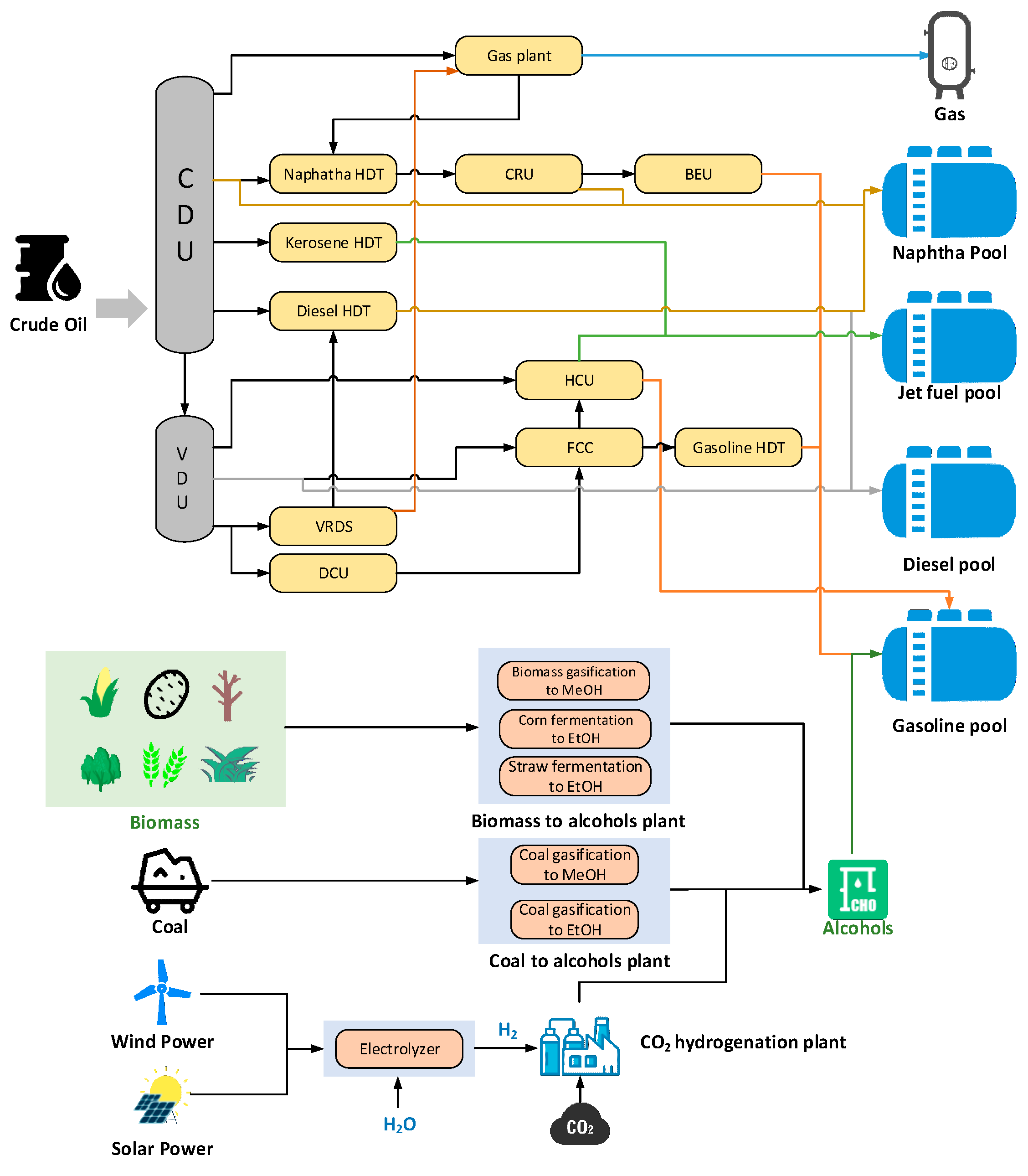
Figure 1. Benchmark process flow.
Processes 12 01751 g001
Figure 2. The topological structure of the gasoline blending ELM model.
Processes 12 01751 g002
Figure 3. Carbon footprint tracking flowchart.
Processes 12 01751 g003
Figure 4. Comparison of predicted RON by different methods.
Processes 12 01751 g004
Figure 5. The gross margin (GM) of refineries with alcohol blending.
Processes 12 01751 g005
Figure 6. Gasoline carbon footprint.
Processes 12 01751 g006
Figure 7. Composition of gasoline carbon footprint.
Processes 12 01751 g007aProcesses 12 01751 g007b
Figure 8. Cost trend of alcohols.
Processes 12 01751 g008
Figure 9. Base BEV of case refineries.
Processes 12 01751 g009
Figure 10. BEV trend of case refineries (Blending Level = 20%).
Processes 12 01751 g010
Figure 11. Comparison of BEV and cost (Blending Level = 20%).
Processes 12 01751 g011aProcesses 12 01751 g011b
Figure 12. GM trend of case refineries (Blending Level = 20%).
Processes 12 01751 g012
Figure 13. GM by alcohol blending level (Fixed Operating Year = 2050).
Processes 12 01751 g013
Figure 14. CF by alcohol blending level (Fixed Operating Year = 2050).
Processes 12 01751 g014
Table 1. Summary of recent research on blending optimization techniques.
StudyMethod(s) UsedKey Results
Sun et al. [44]Random Forest Achieved a maximum prediction error of 0.46 for Research Octane Number (RON), closely aligning with experimental uncertainty.
Ibrahim et al. [45]Artificial Neural Network (ANN)Demonstrated effective modeling of hydrocarbon mixtures and gasoline–EtOH blends, capturing nonlinear octane rating relationships using infrared spectroscopy data.
Li et al. [47]Group Contribution Method (GCM)Successfully predicted RON for both pure fuel compounds and blends
Zhang et al. [48]Robust machine learningPredicted RON loss and sulfur content during refining with high accuracy and strong generalization.
Alboqami et al. [49]Genetic Algorithms (GA); ANNDeveloped an optimized method for predicting fuel octane ratings, effectively minimizing the use of high-octane components.
Wang et al. [50]Extreme Learning MachineCompared the performance of various ELM approaches, highlighting their effectiveness in different scenarios.
Table 2. Raw materials and product prices.
MaterialsCost and Price, CNY/tCarbon Footprint, kgCO2/t
CtM19536580
BioM3500370
CCUM8400−540
CornE47001020
StrawE55882010
CtE40715880
Saudi Medium Crude Oil3480——
Gasoline4775——
Jet fuel4767——
Diesel4281——
Aromatics6075——
LPG2787——
Petroleum Coke1383——
Table 3. Comparison of prediction errors.
MethodsMSEMAERMSER2
ELM0.03160.17000.17830.8423
Linear blending0.07960.23600.28210.6054
Disclaimer/Publisher’s Note: The statements, opinions and data contained in all publications are solely those of the individual author(s) and contributor(s) and not of MDPI and/or the editor(s). MDPI and/or the editor(s) disclaim responsibility for any injury to people or property resulting from any ideas, methods, instructions or products referred to in the content.