Deciphering Rod Pump Anomalies: A Deep Learning Autoencoder Approach

Abstract

This paper investigates the application of a self-coder neural network in oilfield rod pump anomaly detection. Rod pumps are critical equipment in oilfield production engineering, and their stability and reliability are crucial to the production efficiency and economic benefits. However, rod pumps are often affected by anomalies such as wax deposition, leading to increased maintenance costs and production interruptions. Traditional wax deposition detection methods are inefficient and fail to provide early warning capabilities. This paper reviews the research progress in sucker rod pump anomaly detection and autoencoder neural networks, providing a detailed description of the construction and training process of the autoencoder neural network model. Utilizing data from the rod-pumped wells of the Tuha oilfield in China, this study achieves the automatic recognition of various anomalies through data preprocessing and the training of an autoencoder model. This study also includes a comparative analysis of the differences in the anomaly detection performance between the autoencoder and traditional methods and verifies the effectiveness and superiority of the proposed method.

1. Introduction

As a type of artificial lifting equipment widely used in oilfield oil recovery engineering, the stability and reliability of rod pumps’ operation directly affects the production efficiency and economic benefits of the oilfield [1]. However, in practical application, rod pumps are often affected by waxing and other abnormalities, which not only increase the maintenance cost but also may lead to production interruptions, resulting in serious economic losses. Wax deposition refers to the process during which paraffinic substances accumulate on the surfaces of a sucker rod pump, forming a wax layer. Over time, as this layer thickens, it can lead to a reduction in pump efficiency and, in severe cases, complete blockage. Traditional methods for the detection of wax deposition rely on regular inspections and maintenance. These methods are not only inefficient but also typically identify issues only after they become apparent, failing to provide early warnings [2].

In recent years, with the rapid development of artificial intelligence and machine learning technologies, autoencoder neural networks, as an unsupervised learning method, have attracted attention for their potential in the field of abnormality detection. Autoencoders are able to identify abnormal behaviors that deviate from normal patterns by learning the data distribution under normal operating conditions, providing new ideas for the real-time monitoring and early failure warning of rod pumps. Although autoencoder neural networks have performed well in anomaly detection in other fields, there are relatively few applications in rod pump anomaly detection [3,4]. In light of this, the present study aims to explore the application of autoencoder neural networks in the anomaly detection of rod pumps, with the expectation of enhancing the accuracy and real-time capabilities of detection, thereby reducing potential risks in oilfield production.

This study firstly provides a comprehensive review of the advancements in rod pump anomaly detection and autoencoder neural network research and then describes the construction and training process of an autoencoder neural network model in detail. In addition, this study compares and analyzes the differences in the anomaly detection performance between the autoencoder neural network and the traditional method, which verifies the effectiveness and superiority of the proposed method.

2. Methodology

2.1. Rod Pump Data

In the Tuha oilfield in China, as a key piece of oil recovery equipment, the monitoring of the rod pumps’ operation status is crucial to ensure the efficient production of the oilfield. To achieve this objective, we have collected a vast array of surface parameter data from rod pump wells in the oilfield, which include not only dynamic data and static data but also historical operation and maintenance records. Dynamic data, such as the displacement, load, current, voltage, and power parameters, are obtained by data acquisition for each up-and-down stroke cycle of the rod pump, and the real-time nature of these data provides the possibility of analyzing the instantaneous state of the pump [5]. Meanwhile, static data, such as the rod and column structure and equipment configuration parameters, do not vary over time, but they provide a foundation for an understanding of the long-term performance and stability of the pump. In addition, historical data reflect past operations and maintenance, providing valuable information for the analysis of long-term pump performance trends and maintenance needs. This collection of data embodies the concept of “big data,” and its vast volume provides a solid foundation for the extraction of critical information and the evaluation of rod pump operating systems. Through the in-depth analysis of this data, we can better understand the operating status of rod pumps, identify potential failure modes, and achieve the real-time monitoring of pump health.

We performed a thorough review of the original dataset to identify and correct potential data entry errors. Through logical checks and validation by domain experts, we eliminated duplicate records and filled in missing values [6]. Missing values were addressed using a variety of techniques, including the mean, the median, seasonal interpolation, and, where appropriate, multiple interpolation methods. To address the effects of different scales and magnitudes, we standardized all numerical features. The z-score standardization was used with the aim of removing the effects of different scales and magnitudes and giving the data a uniform scale. Finally, we divided the cleaned and standardized dataset into a training set and a test set to evaluate the performance of the model. The training set was used for the estimation of the model parameters, while the test set was used to verify the generalization ability of the model [7,8]. These preprocessing steps are crucial for subsequent data analysis and model construction as they ensure the consistency and reliability of the dataset. Using the cleaned and normalized data, we constructed a self-encoder neural network model for fault identification and health monitoring via anomaly detection methods. This model is capable of learning the data patterns of a rod pump during normal operation and identifying abnormal behaviors that deviate from these patterns, enabling the early warning of potential problems such as wax formation, as depicted in Figure 1. In addition, by analyzing the output of the model, we can predict when certain conditions will occur and identify the key decision variables that lead to failures, providing valuable insights and decision support to oilfield operators.

By statistically analyzing and visualizing the data, we are able to more intuitively understand the operational status and performance trends of rod pumps. Charts and graphs not only help us to identify patterns and anomalies in the data, but also provide an effective means to communicate the results of complex data analysis to non-technical stakeholders. The application of this integrated approach allows us to provide data-based decision support for rod pump maintenance and operation, thereby improving the oilfield’s productivity and safety.

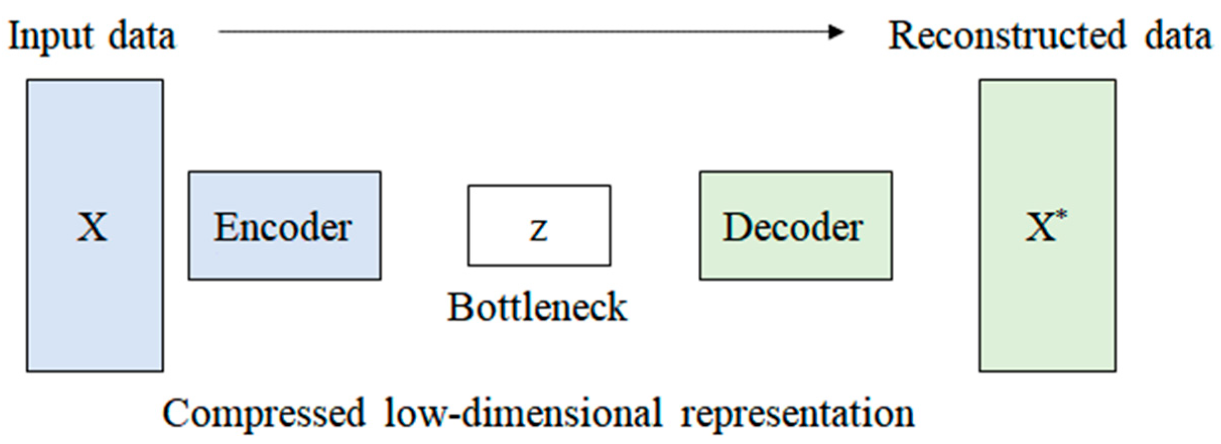
2.2. Autoencoder Model

An autoencoder is a neural network that encodes and decodes data through unsupervised learning, with the goal of learning an efficient representation or characterization of the data. Autoencoders usually consist of two parts: an encoder and a decoder [9,10,11]. The encoder compresses the input data into a low-dimensional representation, while the decoder reconstructs this low-dimensional representation back into the original data, as depicted in Figure 2. During training, the network tries to minimize the difference between the input and the reconstruction.

The raw data x are encoded from the input layer to the hidden layer:

$$h_i=f_i(h_{i-1})$$

(1)

where h_x is the activation value of layer i, and h₀ = x is the input data.

The bottleneck layer z is the output of the encoder and a potential representation of the autoencoder:

$$z=f_{\mathrm{bottleneck}}(h_{\mathrm{encoder} \mathrm{last}})$$

(2)

This layer typically uses activation functions such as tanh or ReLU to increase the model’s nonlinear fitting capabilities.

The decoder carries out the inverse process of the encoder, mapping the latent representation z back to the original data dimensions.

Here, g represents a series of functions of the decoder and x* is the reconstructed output.

$$x^{*}=g(z)$$

(3)

The training objective of an autoencoder is to minimize the difference between the input x and the reconstruction x*. This is typically achieved through the use of the mean squared error (MSE) loss function.

$$L=\Vert x-x^{*}{\Vert }_2^2$$

(4)

where ‖-‖² represents the Euclidean norm.

To minimize the loss function L, we use an optimization algorithm such as stochastic gradient descent (SGD) or its variant, adaptive momentum with the stochastic optimization method and the Adam optimizer, to update the weights of the network [12].

The training process consists of forward propagation, the computation of the loss, the backpropagation of the error, and the updating of the weights. This process can be represented as

$${\theta }_{\mathrm{new}}={\theta }_{\mathrm{old}}-\eta {\nabla }_{\theta }L$$

(5)

where θ represents the parameters of the model, η is the learning rate, and ∇_θL is the gradient of the loss function with respect to the parameters.

After the training is completed, the autoencoder can be used for anomaly detection. The threshold ϵ for anomaly detection can be determined based on the distribution of the reconstruction error [13]. When L is greater than ϵ, it is considered to indicate anomalous data.

2.3. Dynamic Threshold Calculation Method

In the field of anomaly warning for rod pumps, the dynamic threshold updating strategy is particularly important when applying autoencoder neural networks for anomaly detection [14]. As a powerful feature extraction tool, the autoencoder is able to learn the intrinsic representation of the data and recognize anomaly patterns that are significantly different from the training data during the reconstruction process. However, with the continuous changes in the operating conditions of rod pumps, fixed thresholds may not accurately capture all potential anomalies, necessitating a dynamic thresholding mechanism that can adapt to process changes [15].

The concept of dynamic thresholding represents an innovative adaptive mechanism in the field of statistics and machine learning; it can dynamically adjust to real-time data, maintaining the accuracy and efficiency of an anomaly detection system [16]. This mechanism is particularly applicable to oil recovery systems that require real-time monitoring, where data streams emerge in a continuous and ever-changing manner. In real-time monitoring systems, the dynamic nature of the data necessitates an anomaly detection model that can adapt to changes in statistical characteristics [17]. Dynamic thresholding provides a flexible solution for anomaly detection by capturing new trends and patterns in the data stream. This approach not only improves the accuracy of the system but also enhances its adaptability to new situations, reducing false alarms and omissions that fixed thresholds can cause.

As a key component of dynamic threshold calculation, the moving average is a widely used tool in time series analysis [18]. It is obtained by calculating the average of the data points over a specified time window to smooth the data and reduce the impact of random fluctuations. The mathematical expression of this method is usually as follows:

$${\mathrm{MA}}_t={\displaystyle \frac{1}{w}}{\displaystyle \sum _{i=t-w+1}^t{x}_i}$$

(6)

where MA_t is the moving average of time point t. w is the size of the time window, and x_i is the raw data value at the i-th time point in the time series.

The standard deviation is a statistic that measures the degree of dispersion of the data distribution. It is used to assess the variability of the data. The calculation method for the moving standard deviation is as follows:

$${\mathrm{SD}}_t=\sqrt{{\displaystyle \frac{1}{w-1}}{\displaystyle \sum _{i=t-w+1}^t{(x_i-{\mathrm{MA}}_t)}^2}}$$

(7)

where SD_t is the moving standard deviation at time point t.

Incorporating both the moving average and standard deviation allows for the dynamic calculation of thresholds for anomaly detection. The thresholds can be computed using the following formula:

$${ϵ}_t={\mathrm{MA}}_t+k\times {\mathrm{SD}}_t$$

(8)

where t is a dynamic threshold at time point t and k is a constant that can be adjusted according to the specific needs of the system.

The threshold update strategy means that the threshold can be updated with each new observation of the data stream. This approach ensures that the thresholds are always aligned with the most recent data characteristics. If the reconstruction error of real-time data surpasses the dynamic threshold, the system flags it as a potential anomaly, thereby reducing the incidence of false alarms and omissions that can occur with fixed thresholds. In practical applications, an automated mechanism is necessary to calculate and update these thresholds. This can be efficiently achieved through a software algorithm that regularly receives new data points and adjusts the thresholds accordingly. It is essential to evaluate the performance of the dynamic threshold calculation method to ensure its accuracy in detecting anomalies under diverse conditions [19].

3. Case Study

In this study, a typical rod pump well in the Tuha oilfield in China was selected as a case study object and was visualized in detail, as shown in Figure 3. This well is deemed to have significant research value due to its abnormalities during historical operation and its complete operation and maintenance records. Through the in-depth analysis of the well’s operation data, this study aimed to verify the ability of autoencoder neural networks to detect abnormalities in actual oilfield production and to explore their potential application in the field of fault warning.

The data log encompasses a range of parameters, including the downhole pump depth, oil pressure, casing pressure, dynamic fluid level, load, displacement, current, voltage, and power. Additionally, the data records provide critical information on the time of failure for each well. Data are collected hourly.

In this study, we employed the Linux operating system as our experimental platform, leveraging its excellent multitasking capabilities and stability to provide an ideal execution environment for complex computational tasks. The experimental hardware configuration includes a central processing unit (CPU) with four cores and a powerful Tesla V100 graphics processing unit (GPU). This setup ensures that, during the execution of deep learning and other computer-intensive tasks, we can achieve efficient parallel processing capabilities and significant acceleration effects.

In the experimental process, we conducted iterative training on data collected from the equipment under normal operating conditions. This training phase is crucial for the model to learn and gradually adapt to the characteristics of the data. To assess the model’s performance during training, we utilized the loss function defined in Equation (4) as the optimization target. The loss function, a mathematical metric measuring the discrepancy between the model’s predictions and the actual observations, is vital in adjusting the model parameters during training. Through continuous iterative training, the prediction error of the model gradually decreases until it reaches an acceptable minimum value, indicating that the model has converged. The visualization of the convergence process is shown in Figure 4, which documents in detail the gradual decrease in the loss function value as the number of iterations increases and converges. To avoid overfitting the model and to optimize its performance, a series of trial and error adjustments were implemented. This process involved the careful identification and selection of data points by the model, with a particular focus on those data points that exhibited the highest uncertainty or had the greatest error reduction potential. These data points, due to their critical role in improving the model performance, were prioritized for selection and submitted to domain experts for precise labeling. This active learning strategy ensures that the reliability of the model is effectively assessed during the training process.

Production data from stable regions were normalized and used as input matrices to construct a robust encoder model. Additionally, historical data corresponding to periods of instability or failure were selected to form a test dataset, which was then provided to the encoder model. This process can be repeated for historical events that lead to failures. An encoder anomaly detection model was built to predict the time of failure. The potential anomalous times before a pump shaft breakage were identified by applying reconstruction errors.

Using Well A as a case study, we calculate the reconstruction error, as illustrated in Figure 5. In the event of wax deposition, the detection results, which are based on the discrepancies between the model’s predictions and the actual observations during normal conditions, are employed to ascertain the timing for well suspension.

We compare the actual downtime recorded from well workover operations in the oilfield with the prediction of wax formation by the anomaly detection model. The analysis of

Table 1. Comparison of model-predicted and actual downtime for waxing conditions in rod pump.

Case	Anomaly Detection Model Prediction Time	True Failure Time
Well A	20 July 2023 08:30	21 July 2023 10:00
Well B	14 August 2023 14:15	15 August 2023 16:00
Well C	10 September 2023 20:00	11 September 2023 01:30
Well D	02 November 2023 18:00	05 November 2023 15:20

indicates that the model’s predictions regarding the well shutdown times are slightly earlier than the actual occurrences. Consequently, the anomaly detection model demonstrates a high degree of accuracy in forecasting the timing of rod pump shutdowns due to wax deposition. The autoencoder technology can serve as the foundation for the development of improved autoencoder-based fault prediction tools [20].

4. Conclusions

This study successfully explores the application of an autoencoder neural network in rod pump anomaly detection, enhancing the accuracy and real-time capabilities of the detection process and reducing potential risks in oilfield production. Through case studies, the ability of autoencoder neural networks to detect anomalies in real oilfield production is verified, and their potential application in the field of fault warning is explored. The application of the dynamic threshold calculation method improves the accuracy and efficiency of the anomaly detection system and reduces false alarms and omissions. The experimental results show that the autoencoder neural network can effectively predict potential problems such as wax deposition, providing valuable insights and decision support for oilfield operators. Therefore, the autoencoder technology can be utilized not only as an unsupervised machine learning technique for the real-time prediction of wax deposition in rod pumps, but also as a foundation for the development of more advanced fault prediction tools.

References

1. Wang, Z.; Dong, Y.; Zheng, X.; Wang, X.; Gao, P.; Zhang, L.; Huang, Y.; Sun, W.; Zhang, P. A Deep Learning Model to Intelligently Identify the Working Status of Screw Pumps for Oil Well Lifting. In Proceedings of the SPE/IATMI Asia Pacific Oil & Gas Conference and Exhibition, Virtual, 12–14 October 2021; p. D011S009R007. [Google Scholar]
2. Ramírez, C.; Espinola, O.; Álvarez, J.; Torres, A.; Avena, J.; Basilio, I.; Guerrero, C. A Digitalized New Life For a 100 Year-Old Heavy Oil Brown Field. In Proceedings of the SPE Trinidad and Tobago Section Energy Resources Conference, Port of Spain, Trinidad and Tobago, 25–26 June 2018; p. D011S007R003. [Google Scholar]
3. Szladow, A.J.; Mills, D.; Yong, D. Application of Intelligent System (DES PCP) For Monitoring Progressing Cavity Pumps. In Proceedings of the Canadian International Petroleum Conference, Calgary, AB, Canada, 10–12 June 2003. [Google Scholar]
4. Bangert, P. Diagnosing and Predicting Problems with Rod Pumps Using Machine Learning. In Proceedings of the SPE Middle East Oil and Gas Show and Conference, Manama, Bahrain, 18–21 March 2019. [Google Scholar]
5. Knafl, M.; Prosper, C.; Hoday, J.; Braas, M. Diagnosing PCP Failure Characteristics Using Exception Based Surveillance in CSG. In Proceedings of the SPE Progressing Cavity Pumps Conference, Calgary, AB, Canada, 26–27 August 2013; p. SPE-165655-MS. [Google Scholar]
6. Gupta, S.; Nikolaou, M.; Saputelli, L.; Bravo, C. ESP Health Monitoring KPI: A Real-Time Predictive Analytics Application. In Proceedings of the SPE Intelligent Energy International Conference and Exhibition, Aberdeen, Scotland, UK, 6–8 September 2016; p. SPE-181009-MS. [Google Scholar]
7. Espin, D.A.; Gasbarri, S.; Chacin, J.E. Expert System for Selection of Optimum Artificial Lift Method. In Proceedings of the SPE Latin America/Caribbean Petroleum Engineering Conference, Buenos Aires, Argentina, 27–29 April 1994. [Google Scholar]
8. Liu, Y.; Yao, K.; Lenz, T.L.; Olabinjo, L.; Seren, B.; Seddighrad, S.; Babu, C.G.D. Failure Prediction for Rod Pump Artificial Lift Systems. In Proceedings of the SPE Western Regional Meeting, Anaheim, CA, USA, 27–29 May 2010. [Google Scholar]
9. Liu, Y.; Yao, K.-T.; Raghavenda, C.S.; Wu, A.; Guo, D.; Zheng, J.; Olabinjo, L.; Balogun, O.; Ershaghi, I. Global Model for Failure Prediction for Rod Pump Artificial Lift Systems. In Proceedings of the SPE Western Regional & AAPG Pacific Section Meeting 2013 Joint Technical Conference, Monterey, CA, USA, 19–25 April 2013; p. SPE-165374-MS. [Google Scholar]
10. Boguslawski, B.; Boujonnier, M.; Bissuel-Beauvais, L.; Saghir, F.; Sharma, R.D. IIoT Edge Analytics: Deploying Machine Learning at the Wellhead to Identify Rod Pump Failure. In Proceedings of the SPE Middle East Artificial Lift Conference and Exhibition, Manama, Bahrain, 28–29 November 2018; p. D021S004R001. [Google Scholar]
11. Zukoski, E.E. Influence of Viscosity, Surface Tension, and Inclination Angle on Motion of Long Bubbles in Closed Tubes. J. Fluid Mech. 1966, 25, 821–837. [Google Scholar] [CrossRef]
12. Chen, Y.-T.; Zhang, D.-X.; Zhao, Q.; Liu, D.-X. Interpretable Machine Learning Optimization (InterOpt) for Operational Parameters: A Case Study of Highly-Efficient Shale Gas Development. Pet. Sci. 2023, 20, 1788–1805. [Google Scholar] [CrossRef]
13. Siddique, M.F.; Ahmad, Z.; Kim, J.-M. Pipeline Leak Diagnosis Based on Leak-Augmented Scalograms and Deep Learning. Eng. Appl. Comput. Fluid Mech. 2023, 17, 2225577. [Google Scholar] [CrossRef]
14. Bangert, P. Predicting and Detecting Equipment Malfunctions Using Machine Learning. In Proceedings of the SPE Middle East Oil and Gas Show and Conference, Manama, Bahrain, 18–21 March 2019. [Google Scholar]
15. Hasan, A.R.; Kabir, C.S. Predicting Multiphase Flow Behavior in a Deviated Well. SPE Prod. Eng. 1988, 3, 474–482. [Google Scholar] [CrossRef]
16. Ma, H.; Han, G.; Peng, L.; Zhu, L.; Shu, J. Rock Thin Sections Identification Based on Improved Squeeze-and-Excitation Networks Model. Comput. Geosci. 2021, 152, 104780. [Google Scholar] [CrossRef]
17. Rathnayake, S.I.; Firouzi, M. Statistical Process Control for Early Detection of Progressive Cavity Pump Failures in Vertical Unconventional Gas Wells. In Proceedings of the 2021 Asia Pacific Unconventional Resources Technology Conference, Unconventional Resources Technology Conference, Online, 16–18 November 2021. [Google Scholar]
18. Khadav, S.; Agarwal, S.; Kumar, P.; Pandey, N.; Parasher, A.; Kumar, S.; Agarwal, V.; Tiwari, S. System Run Life Improvement for Rod Driven PCP in High Deviation Well. In Proceedings of the SPE Artificial Lift Conference and Exhibition-Americas, The Woodlands, TX, USA, 28–30 August 2018; p. D012S002R004. [Google Scholar]
19. Hasan, A.R.; Kabir, C.S. Two-Phase Flow in Vertical and Inclined Annuli. Int. J. Multiph. Flow 1992, 18, 279–293. [Google Scholar] [CrossRef]
20. Al-shammari, B.S.; Rane, N.; Ali, S.M.; Sultan, A.A.; Al Sabea, S.H.; Al-naqi, M.; Pandey, M.; Solaeche, F.L. Using Real-Time Data and Integrated Models to Diagnose Scale Problems and Improve Pump Performance. In Proceedings of the SPE Middle East Oil and Gas Show and Conference, Manama, Bahrain, 15 March 2019; p. D032S085R003. [Google Scholar]
Figure 1. Available rod pump data.
Processes 12 01845 g001
Figure 2. Architecture of autoencoder.
Processes 12 01845 g002
Figure 3. Operational history of well A—indicator diagram (The current state in red and the numerous historical states in grey).
Processes 12 01845 g003
Figure 4. Encoder convergence iteration curve.
Processes 12 01845 g004
Figure 5. Reconstruction error used to predict failure time of well A pump.
Processes 12 01845 g005