Article

Numerical Simulation of Salmon Freezing Using Pulsating Airflow in a Model Tunnel

by
Edgardo J. Tabilo
1,
Roberto Lemus-Mondaca
1,*,
Luis Puente
1,2 and
Nelson O. Moraga
3
1
Department of Food Science and Chemical Technology, Faculty of Chemical Sciences and Pharmaceutical, Universidad de Chile, St. Dr. Carlos Lorca Tobar 964, Independencia, Santiago 8380000, Chile
2
Department of Agricultural, Food & Nutritional Science, University of Alberta, Edmonton, AB T6G 2P5, Canada
3
Department of Mechanical Engineering, Faculty of Engineering, Universidad de La Serena, Av. Benavente 980, La Serena P.O. Box 9801720160, Chile
*
Author to whom correspondence should be addressed.
Processes 2024, 12(9), 1852; https://doi.org/10.3390/pr12091852
Submission received: 2 August 2024 / Revised: 22 August 2024 / Accepted: 26 August 2024 / Published: 30 August 2024
(This article belongs to the Special Issue Production Planning, Modeling and Control of Food Industry Processes)

Abstract

:

Highlights

What are the main findings?
  • CFD conjugate model for improved salmon freezing in a tunnel with a pulsed airflow
  • Pulsating airflow freezing allowed important energy savings compared to steady flow
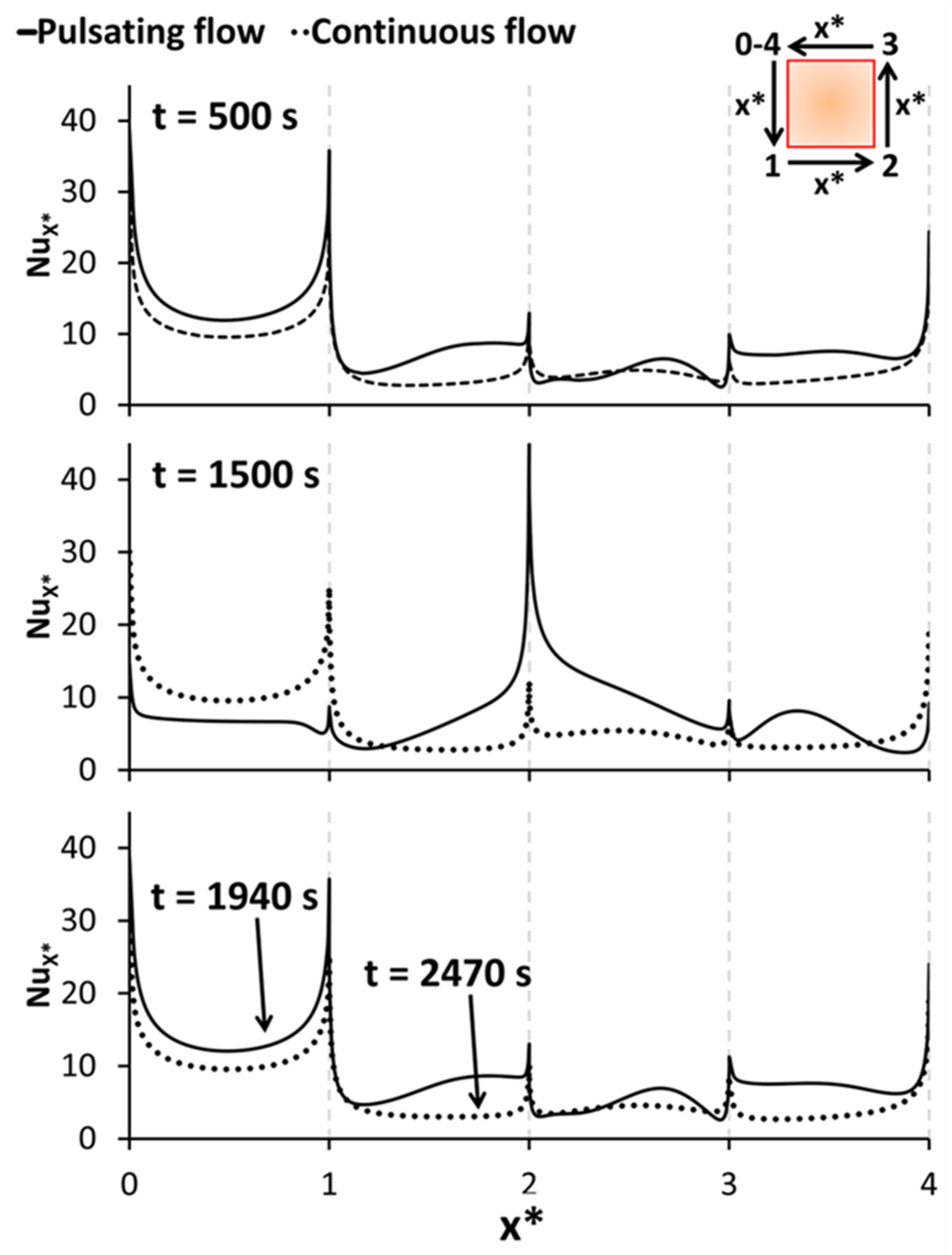
  • Higher Nusselt number in food and faster freezing achieved by pulsed inlet airflow
  • Fast numerical predictions and third-order accuracy calculation of transient terms
  • High-quality freezing of solid food in mixed convective heat refrigeration tunnel

Abstract

Food freezing is an energy-intensive thermal process that has required exploring new technologies to enhance productivity and efficiency. This work provides a detailed insight into the energy analysis for the improved cooling of solid food during the freezing process, which originated by imposing a pulsating airflow at the entrance of a convective freezer tunnel. Continuity, linear momentum, and energy equations described simultaneously the conjugate transient heat conduction with liquid-to-solid phase change of the water content of a square salmon piece and the unsteady heat transfer by mixed convection in the surrounding airflow. The Finite Volume Method and a recently developed fast-accurate pressure-correction algorithm allowed an accurate prediction for the effects of imposing an inlet pulsating cooling airflow on the evolution of vortex-shedding, food freezing, cooling rate, heat flow, and energy savings. The variation in the values of the local heat fluxes at the food surface was reported, analyzed, and discussed by the evolution of the local Nusselt number around the square salmon piece. The study found that using an inlet pulsed airflow during salmon freezing improved temperature distribution and reduced energy consumption by 21% compared to using an inlet constant velocity airflow. The findings conclude that using pulsed airflow can improve temperature distribution in the food and significantly reduce energy consumption. Future investigations should consider a three-dimensional analysis, real salmon shape, turbulent conjugate convective freezing, an ensemble of salmon pieces, and exergy analysis to improve freezing tunnel design.

1. Introduction

Refrigeration accounts for almost one-quarter of the electricity consumption worldwide [1]. At the same time, freezing is the most intensive thermal process in energy use due to the liquid-to-solid phase change that originates from cooling the water content in foods [2]. Freezing is a thermal preservation method that reduces food water activity, inhibits microbial growth activity, and decreases the chemical reaction rate, increasing food shelf-life [3]. The growth rate of the ice crystals generated by the solidification of the water content in the food material intercellular region must be controlled to guarantee fast freezing able to create smaller ice crystals, decreasing cell damage and reducing the changes in food color and texture [4].
Air blast freezing is a low operational cost method applied in large-size refrigeration tunnels, allowing the processing of a high volume of products. Electrical energy consumption is high because the air temperature range used in this process varies between −35 °C and −52 °C. In this technology, the freezing rate depends on the air temperature and velocity, food properties, shape and dimensions, position of products, and refrigerator tunnel design [5]. Multiple studies have been developed to improve the productivity of this process, which allows for decreasing the processing time without food quality loss caused by freezing conditions [6]. Alam and Kim (2018) [7] classified heat transfer enhancement techniques into passive and active methods. The dynamic methods require adding external energy to the original system.
In contrast, passive methods do not require energy injection and are based on surface modification or insertion of turbulence-generating elements in the coolant flow [8]. Pulsating flow is considered an active method since the pulsating or oscillating motion of the cooling fluid disturbs the thermal boundary layer, inducing turbulence and instability in the flow and enhancing heat transfer [9]. Ye et al. (2021) [10] summarized the different types of pulsating flow: single-phase pulsating flow, two-phase pulsating flow, and intermittent jet impingement. Various researchers have focused on the study of single-phase pulsating flows, which include laminar pulsating flow in channels [11,12], flow around objects [13,14,15], pulsating fluid flow through porous media [16], single-phase nanofluid pulsating flow [17], and pulsating flow around ribs [18,19]. The current research proposal centers on the study of pulsating airflow fluid dynamics and heat transfer around an object, specifically a square-shaped piece of salmon.
In recent decades, computational fluid dynamics has significantly optimized equipment design, process improvement, and experiment design, reducing the need for physical experiments and the associated costs of experimentation and raw materials [20,21,22,23]. The main advantage of numerical simulations is that the evolution of the distribution of the dependent variables (velocity, pressure, and temperature) and derived variables, such as heat fluxes or shear stresses, can be predicted quickly and accurately [24,25,26,27]. The conjugate models of fluid mechanics and heat transfer enable the simultaneous determination of fluid dynamics and heat flow from the food to the cooling fluid. This feature identifies critical areas for improving thermal process efficiency and eliminates the need for a semi-empirical model for calculating convective heat transfer coefficients [28,29,30]. Understanding the physical properties of food and materials involved in freezing is essential for resolving mathematical model equations. When food undergoes freezing, its thermophysical properties significantly change near the freezing point. The chemical composition of food and the conditions of the process influence these alterations. Therefore, obtaining experimental measurements for the thermal properties under all conditions is impractical. As a practical alternative, the thermal properties of foods can be determined by utilizing reliable, temperature-dependent mathematical models derived from empirical equations based on the thermal characteristics of individual food components. Initially formulated by Choi and Okos, these models remain valid within a temperature range of −40 to 150 °C. Furthermore, they encompass mathematical expressions for predicting water and ice properties within the same temperature range [31,32,33,34].
This study aims to evaluate the effect of pulsating airflow at the tunnel inlet on thermal convective performance during solid food freezing to achieve a high-quality salmon muscle by reduced temperature gradients in the meat. The goal is to achieve more efficient cooling and freezing rates, leading to energy savings, reduced processing time, and increased productivity compared to using a constant velocity airflow at the tunnel inlet. This research stands out due to its incorporation of a conjugate mathematical model. The model addresses unsteady mixed heat convection of pulsating air flow and transient heat conduction with the liquid–solid phase change phenomenon of the water content in a square piece of salmon. Additionally, it considers the temperature-dependent thermal properties, resolved through an enhanced pressure-correction algorithm using the finite volume method. The findings encompass the visualization of flow patterns, temperature distribution within the air in the freezing tunnel, and the determination of drag and lift coefficients around the solid food. Furthermore, the model facilitates the computation of temperature distribution within the food and the progression of ice formation during the freezing process. Lastly, it enables the identification of the slowest freezing point, the calculation of freezing time, and an assessment of energy savings compared to the case with constant velocity inlet airflow.

2. Material and Methods

This section provides a comprehensive overview of the mathematical methods and models utilized in developing the computational model for this research. The Materials and Methods Section encompasses the physical model of the freezing tunnel, model mathematical equations, initial and boundary conditions, thermal properties of food and materials, calculations of dimensionless numbers and energy consumption, and the detailed computational implementation, including numerical methods, mesh and time step studies, validation of the computational model, and a parametric study aimed at identifying the optimal combination of amplitude and pulsating frequencies.

2.1. Freezing Tunnel Model

The tunnel model pertains to the classical fluid mechanics problem in which fluid flows past a square cylinder positioned between two parallel flat plates. Specifically, this tunnel model was developed by Yu et al. in 2014 [35] to examine the impact on flow and heat transfer characteristics for sinusoidal pulsating laminar flow within a heated square cylinder. In the present study, the heated square cylinder was substituted by a square-shaped portion of salmon, with a side length denoted as B (=1.5 cm), and frozen in a model freezing tunnel with dimensions of LU, LD, and H equal to 10B, 29B, and 20B, respectively, as indicated in Figure 1.

2.2. Mathematical Model Equations

The mathematical model is based on several assumptions, including laminar flow with a Reynolds number of 250 and an initial Grashof number value of 4 × 10⁴. It accounts for negligible viscous dissipation, combined transient natural and forced heat convection, and assumes linear changes in air density with temperature based on the Boussinesq approximation. While the thermophysical properties of the salmon meat change non-linearly with temperature, the model assumes constant air properties, except for density. The model describes the conjugate unsteady fluid mechanics and heat transfer governing the freezing of salmon in the tunnel, represented by Equation (1) of continuity, linear momentum, and energy in the air and inside the salmon meat.
v = 0 ;   ρ v t + v · v = P + μ 2 v + ρ g ;   ρ c p T t + v · T = k 2 T
The determination of thermal properties in frozen foods necessitates the consideration of the ice fraction, which accounts for significant differences between frozen and unfrozen food properties. Below the freezing point, it is essential to consider that the sensible heat and the latent heat of the solidification of water depend on the temperature. Because the latter is released over various temperatures, an apparent specific heat was used to include the effect of sensible and latent heat [36,37]. The expressions that allowed the calculation of density, thermal conductivity, apparent specific heat [38], and ice fraction are stated in Equations (2)–(4) for frozen and unfrozen stages [39],
X i c e = 1.05 · X w o 1 + 0.7138 l n T c f T + 1 ;   x u w = 1 X i c e ;   ρ = 1 / X i / ρ i
c p , u = c p , i · X i ;   c p , a p = 1.55 + 1.26 X s X w o X b w · L o · T c f T 2
k = 1 X i ν / k i ;   X i ν = X i / ρ i X i / ρ i
The procedure for calculating the variation in density, specific heat, and thermal conductivity of salmon meat with temperature, based on empirical equations of thermal properties of the main components of foods, is described in Section 2.4.

2.3. Initial and Boundary Conditions

The initial conditions considered air at rest at −40 °C while the piece of salmon was at 22 °C. The boundary conditions for the fluid mechanics incorporated non-slip at the solid walls, u = v = 0 at y = 0 and at y = H, pulsating air horizontal velocity (Equation (5)) at the tunnel inlet, and a fully developed aerodynamic flow condition, v = 0 and u/ x = 0, at the freezing tunnel outlet (x = L). The Reynolds number was calculated by the inlet average horizontal velocity, Um, and the characteristic length “B” of the square piece of pink salmon
U = U m 1 + A p sin 2 π f p t   at   the   inlet   x = 0 ;   R e = ρ · U m · B μ
Thermal boundary conditions consider a uniform air temperature profile at the tunnel entrance, at x = 0: T(x = 0,t) = −40 °C, adiabatic top and bottom walls; T/ y = 0 at y = 0, and at y = H; and a fully developed thermal state at the tunnel exit, T/ x = 0 at x = L. Conjugation conditions based on the energy conservation principle and continuity of temperature were applied at the salmon-air interfaces (Equation (6)).
k s o l T s o l x i , j i n t = k f l u T f l u x i , j i n t ;   T s o l i n t = T f l u i n t

2.4. Thermophysical Properties

The thermophysical properties of air were acquired through tabulated data covering a temperature range from −40 °C to 25 °C. The obtained data were analyzed to determine the average value of each one, as well as its standard deviation: ρ = 1.312 ± 0.110 kg m−3; Cp = 1006 ± 2 J kg−1K−1; k = 0.0234 ± 0.0017 Wm−1K−1; β = 3.87 ± 0.51 × 10⁻³ K−1 and µ = 1.715 ± 0.108 × 10⁻⁵ Pa s [40]. Thermal properties of the air were assumed to be constant and calculated using the average value within the operational temperature range. The density showed the most significant variation, with an observed deviation of 8% from its average value. The proximal composition of Pink Salmon was determined using the standard AOAC method [38], revealing a moisture content of 76.35%, protein content of 19.94%, fat content of 3.45%, and ash content of 1.22%, with no detectable levels of carbohydrate or fiber. These findings closely corresponded with the USDA tabulated data from the National Nutrient Database for Standard Reference [39]. The thermal properties of the Pink Salmon were calculated in the computational program using the empirical equations for temperature-dependent thermal properties of the food components. These equations were obtained from the most recent review of the Choi and Okos method [31,39,41]. The freezing point of the food denoted as Tcf, is −2.2 °C, and the latent heat of solidification, denoted as L0, is 255 kJ kg−1, per USDA, tabulated data from the National Nutrient Database for Standard Reference [39].

2.5. Calculation of Dimensionless Numbers and Energy Consumption

The drag and lift coefficients around the solid food were determined using Equations (7)–(9) as per the methodology detailed in the paper authored by Yu et al. [35]. Equation (10) details the precise calculation method for determining the dimensionless Nusselt and Strouhal numbers. A second-order accurate approximation was applied to estimate the temperature and velocity gradients, Equation (11). The thermal energy required to freeze the piece of salmon from its initial temperature to the desired freezing temperature was determined by implementing Equation (12). This equation factors in the mass of the food, the sensible heat of the cooling and subcooling stages, the latent heat involved in the phase change, the initial and final temperature of the product, and the duration of the process.
C L = C L P + C L V ; C D = C D P + C D V
C L P = 2 0 B p b p t d x ;   C L V = 2 R e 0 B v x f + v x r d y + v y t + v y b d x
C D P = 2 0 B p f p r d y ;   C D V = 2 R e 0 B u y t + u y b d x + u x f + u x r d y
N u x i , j = d T d x i , j i n t T i n t T B ;   S t = f p · B U m
d ϕ d x i = ϕ k 2 ϕ ϕ k + 1 ϕ k + 2 x i k x i k + 1 x i k x i k + 2 + ϕ k + 1 2 ϕ ϕ k ϕ k + 2 x i k + 1 x i k x i k + 1 x i k + 2 + ϕ k + 2 2 ϕ ϕ k ϕ k + 1 x i k + 2 x i k x i k + 2 x i k + 1
Q ˙ = m f o o d t p r o c e s s c p , u T i n i T c f + L 0 + c p , f r o T c f T f i n

2.6. Computational Implementation

The set of highly non-linear coupled partial differential equations, as represented by Equations (1)–(6), that govern the transport phenomena of the conjugate mathematical model, has been successfully solved using an in-house code based on the Finite Volume Method. The velocity, pressure, and temperature fields were computed within the discretized mathematical model utilizing the enhanced iterative prediction-correction SIMPLERnP algorithm [42]. The convective and diffusive terms of equations for fluid dynamics and heat transport were computed using the Stability-Guaranteed Second-order Difference Scheme (SGSD) [43] and a second-order accurate linear interpolation function [44], respectively. The precise calculation of transient terms encompassing fluid acceleration and the rate of change in internal energy within the mathematical model is enabled with third-order accurate Backward Difference Formulas (BDF3) [45]. The discretized governing equations system was solved using the Bi-Conjugate Gradient Stabilized method (Bi-CGSTAB) [21].
The dependent variables of the mathematical conjugate model were determined using an enhanced pressure prediction-correction iterative procedure. This method allows for the utilization of high sub-relaxation values near unity. The established convergence criteria were as follows: α p = 0.99 for pressure and α u = α v = α T = 0.88 for velocity and temperature, respectively. The SIMPLERnP scheme was designed with an internal cycle comprising of “n” inner iterations to optimize the calculation of the pressure correction and ensure adherence to the discretized continuity equation [42]. The convergence criteria were calculated between consecutive iterations and time steps to ensure the local conservation of mass, momentum, and energy at each control volume. The optimal convergence rate was achieved by employing ten internal cycles to meet the desired criteria values: εSmax = 10−6 and εu = εv = εT = 10−5, for mass, velocity components, and temperature, respectively. The numerical software, programmed in FORTRAN 95/18, was executed on an 11th Gen Intel® Core™ i7-11800H/2.3 GHz personal laptop with 32 GB of RAM.

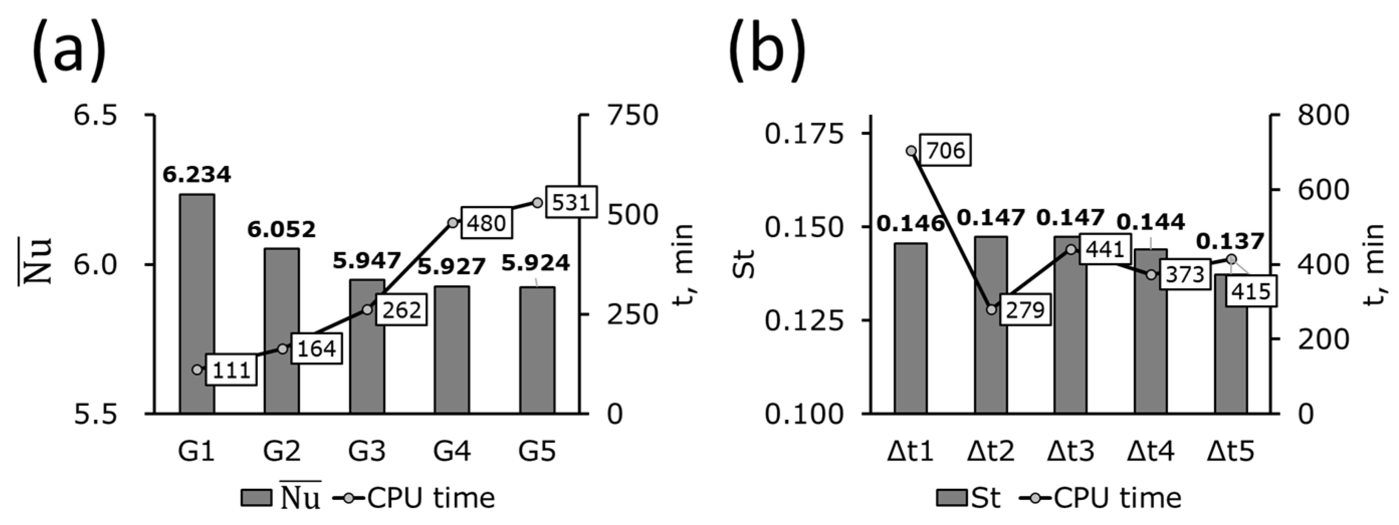
2.6.1. Time and Grid Analysis

The careful selection of the mesh and time step is essential in solving the mathematical model and estimating the relevant variables, such as process time and energy consumption. Following independence tests, the computational domain was discretized using a non-uniform staggered grid consisting of 265 × 200 nodes, with local refinement around the piece of salmon and tunnel walls. Furthermore, a constant time step of 2.0 × 10⁻³ s was utilized to calculate the fluid acceleration and the rate of change in the internal energy in the transient terms of the mathematical model. Figure 2 shows the results of grid and time steps independence tests, carried out by five different grids (G1:133 × 101; G2:182 × 149; G3: 265 × 200; G4: 315 × 240; G5: 365 × 275 nodes) and four values of the time step (Δt1 = 1.0 × 10⁻³ s; Δt2 = 2.0 × 10⁻³ s; Δt3 = 5.0 × 10⁻³ s; Δt4 = 1.0 × 10⁻² s).
In the process of mesh selection, we considered two main criteria: (i) the values of Umax, Vmax, and the average Nusselt number (between the food and air), and (ii) the computational time required to reach 15 s of the process, at which point the vortex-shedding phenomena is in a periodic state. A horizontal profile plotted along the tunnel at y = 10B and a vertical profile passing over the salmon piece at x = 10.5B allowed the calculation of the velocity components along these profiles, which were compared for the five meshes studied (G1:133 × 101; G2:182 × 149; G3: 265 × 200; G4: 315 × 240; G5: 365 × 275 nodes). Upon comparing the meshes, it was observed that the maximum difference in the velocity components was approximately 10−2 m/s, with no discernible trend in their comparison (as shown in Table 1). Mesh selection was primarily influenced by the Nusselt number and CPU time, as depicted in Figure 2a. When comparing mesh G4 (315 × 240 nodes) with mesh G3 (265 × 200 nodes), the difference in Nusselt number decreased from 1.77 to 0.34%, while the computation time increased from 261 to 480 min. Despite the Nusselt number difference falling below 1.8%, the computation time witnessed an 83% increase, leading to the selection of mesh G3 (265 × 200 nodes).
The research in question pertains to studying the physics of the vortex-shedding phenomenon, which results in the periodic behavior of dependent variables within a mathematical model. Some scholarly sources have addressed selecting a time step by employing derivative variables unaffected by minor changes in time, as opposed to the primary variables. In this context, our selection criterion for the time step involved computing the Strouhal number and comparing it with experimental findings documented in specialized literature for a Reynolds number of 250. Okajima [46] reported an experimental Strouhal number, St = 0.143, of the vortex-shedding around a square cylinder with Re = 250. In the present study, the calculated results with four values of time steps varied between St = 0.137, with a time of computation of 415 min when the time step Δt5 = 1.0 × 10⁻² s, and St = 0.147 in 279 min, with a time step Δt2 = 2.0 × 10⁻³ s. Due to the exemplary agreement between our results and the experimental data for the value of the Strouhal number St, we opted for the time step Δt2 = 2.0 × 10⁻³ s due to the additional advantage of considerable savings in computation time, Figure 2b.

2.6.2. Computational Model Validation

To ensure the accuracy and reliability of the results obtained in simulating pulsating fluid flow, it was imperative to conduct a comprehensive validation of the stationary fluid flow. As Fowler et al. (2020) emphasized, a thorough validation step is essential, as demonstrated in their investigation of isothermal fluid flow around a square cylinder at Re = 200 [47]. In the present study, we evaluated the computational unsteady conjugate model. This involved comparing the results generated in this investigation with reliable experimental and numerical data reported in the literature for laminar unsteady airflow around a square isothermal cylinder. Specifically, we focused on the drag coefficient, lift coefficient, and Nusselt number, as well as the dimensionless frequency of vortex shedding behind the solid food, calculated by the Strouhal number. The study examined Reynolds numbers 100, 120, 140, 160, 200, and 250; the results are detailed in Table 2. Our findings offer valuable insights into the accuracy of the computational conjugate model. Unlike existing numerical results, our mathematical model accounted for the effect of buoyancy-driven convection, including combined forced and natural heat convection. The final column of Table 2 demonstrates the current results for each coefficient and dimensionless number considering the influence of buoyancy in air. The data presented in the table emphasize a significant finding: as the Reynolds number increases, the average Nusselt value rises, indicating an increase in the heat flux extracted by the air, which serves as a refrigerant during the cooling process. The Nusselt number displays a 60% improvement between Reynolds numbers of 100 and 250.

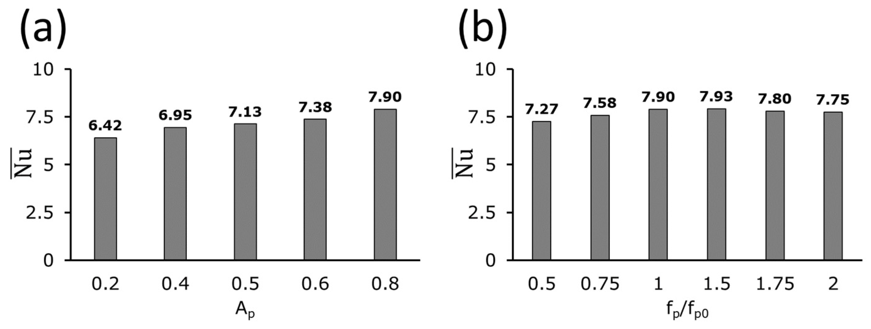
2.6.3. Effects of Pulsating Frequency and Amplitude over Dimensionless Heat Flux

In this segment, an exhaustive parametric study was conducted to ascertain the most adequate combination of pulsating amplitude and frequency, Equation (5). The study focused on a Reynolds number of 250, substituting the salmon piece with an isothermal body. The optimum pairing of pulsating frequency and amplitude was determined to maximize the average Nusselt number around the body, thereby ensuring the highest heat flux extraction by the cooling air. The literature review [35] has revealed that in prior studies, the amplitude of the pulsating airflow ranged from 0.2 to 0.8, allowing for a maximum increase in the inlet velocity of 20 to 80%. In contrast, the pulsating frequency was usually the system’s natural frequency without pulsating flow (fp = fp0). Our study posits that a suitable inlet pulsating airflow can augment the freezing rate. This study comprised two stages of analysis. In the initial stage, the amplitude was systematically varied within the range of 0.2 to 0.8, while the remaining parameters were held constant. The study employed a pulsating frequency ratio, fp/fp0, of 1. Subsequently, in the second stage, the pulsating frequency was systematically varied while maintaining all other parameters constant, utilizing an amplitude, Ap, of 0.8. Figure 3a depicts that a four-times increment of the pulsating amplitude originated an increment of 23% in the Nusselt number. In the case of increasing the pulsating frequency ratio from 0.5 up to 2.0, the graph in Figure 3b illustrated that the average Nusselt number was found to be at its maximum value, Nu = 7.93 when the pulsation frequency was 1.5 times the natural frequency. This finding indicates a 33% increase compared to the steady fluid flow with Re = 250. The research conducted by Moschandreou and Zamir in 1997 [55] examined the impact of pulsatile flow in a tube with a constant heat flux and without an inner solid. The study thoroughly analyzed the influence of the Prandtl number and air pulsation frequency on heat transfer. Their findings revealed a discernible peak in the effect of pulsating frequency, resulting in a substantial increase in the bulk temperature of the fluid and the Nusselt number. When the pulsating frequency falls within a specific range, it triggers a “lock-on” phenomenon, dependent on various parameters such as the Reynolds number and the distance between the square cylinder and the upper and lower walls of the tunnel. Experimental studies indicate that within the “lock-on” zone, an improvement in heat transfer from the square cylinder to the cooling fluid occurs, reaching a maximum value at a certain point before decreasing [56]. The results obtained in the present parametric study closely align with the conclusions drawn from the experimental studies reported in the literature.

3. Results and Discussion

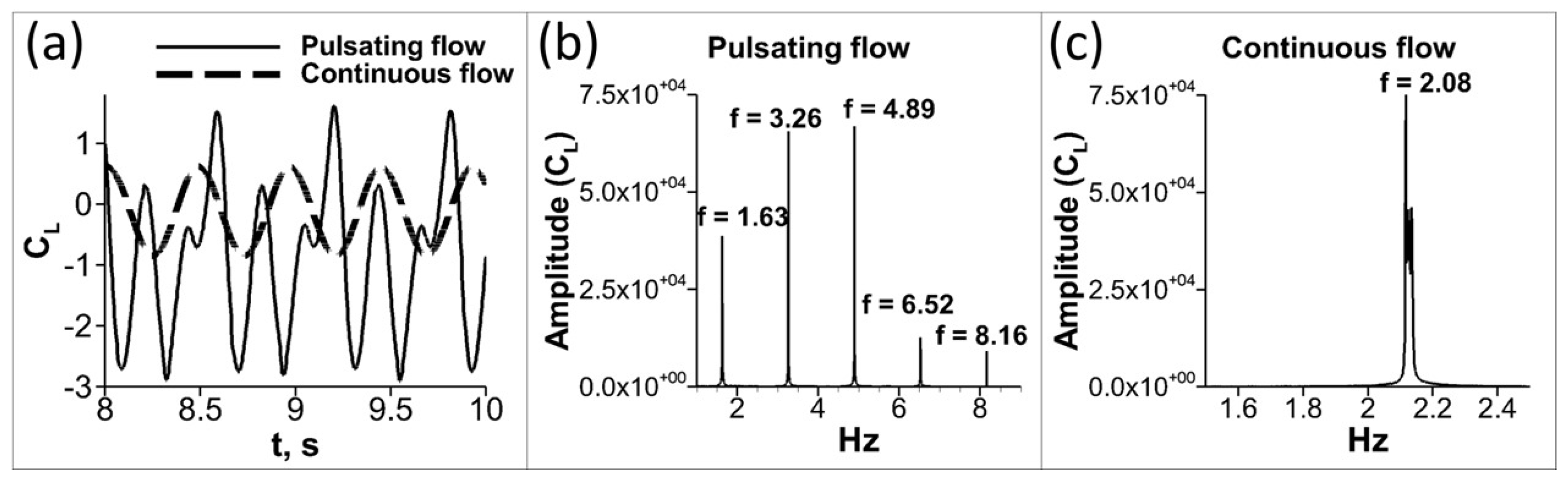
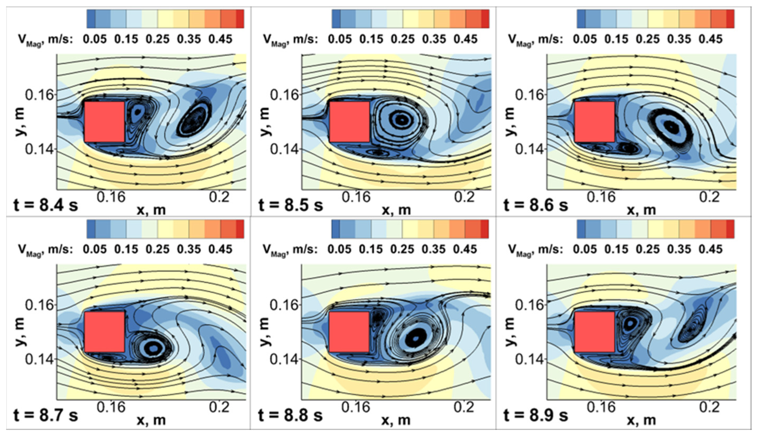
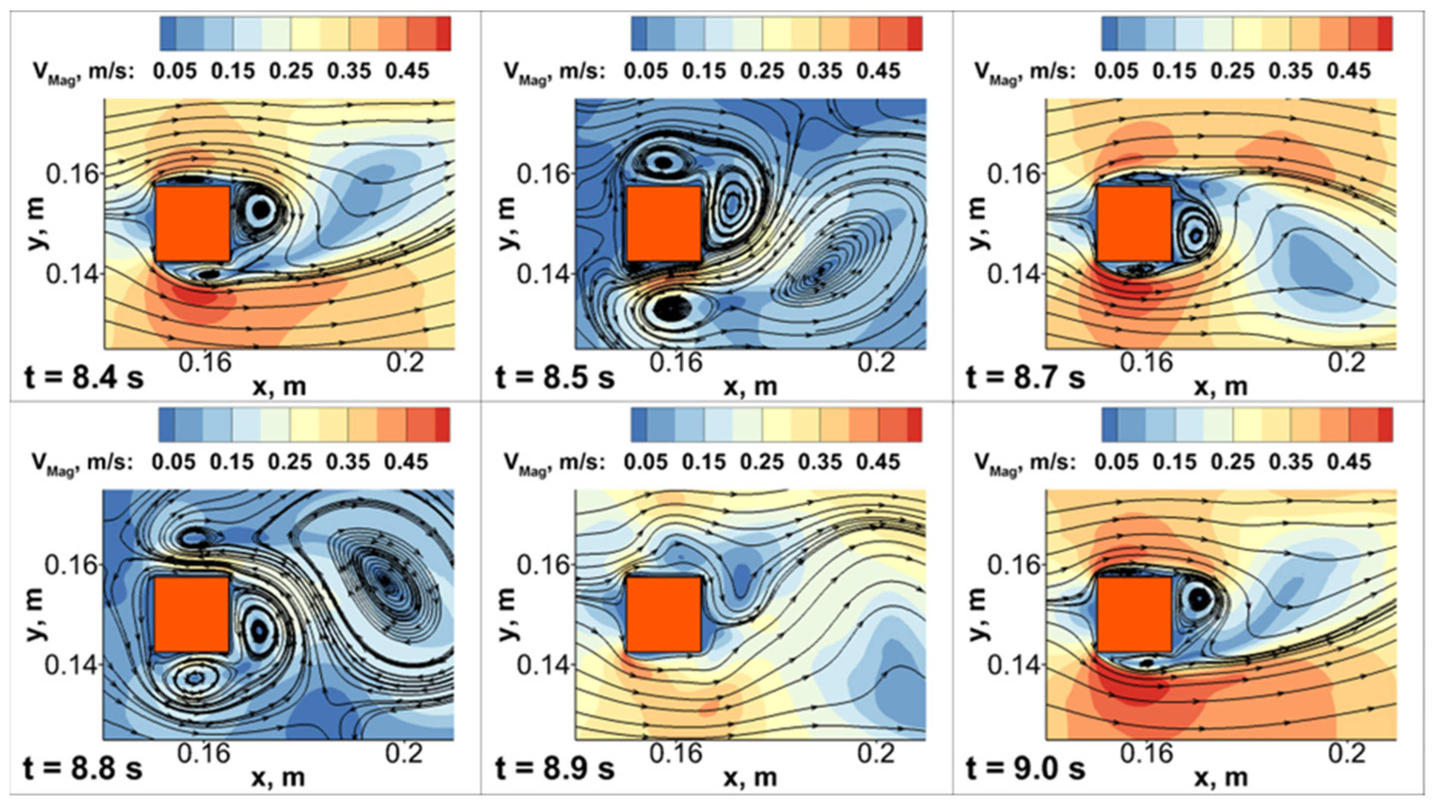
3.1. Effect of Inlet Pulsating Airflow on Fluid Mechanics

The evolution of the lift coefficient demonstrates the wave-like behavior of air flows around a square cylinder. If the air enters the tunnel with a pulsing motion, the lift coefficient exhibits an irregular and repetitive pattern over time, unlike the sinusoidal behavior of steady airflow. The present study combines Ap = 0.8 and fp = 1.5 fp0, where fp0 equals 2.175 Hz, for the pulsating flow, maximizing the Nusselt number. The disturbance of the airflow around the object modifies the boundary layers, which explains the increase in the Nusselt number. Figure 4a shows a higher vortex shedding frequency with pulsating airflow. In Figure 4b,c, the dominant frequency for pulsating inlet flow is twice that of the vortex shedding frequency for the flow with a steady velocity profile. Multiple peaks in Figure 4b represent vortex-shedding frequencies at the horizontal faces and behind the food. Other researchers have observed this behavior [13,14,35]. Saxena et al. [14] studied the pulsating airflow at the inlet around a heated rectangular cylinder for four different aspect ratios. They found that the shape of the lift coefficient evolution curve they observed was similar to that calculated in our investigation at Re = 250, particularly for the square cylinder. They also noted a close agreement between the difference in the magnitude of pulsating and steady inlet flows.
The streamlines around the square piece of salmon caused by vortex shedding with a steady inlet velocity profile are depicted in Figure 5. In contrast, Figure 6 exhibits the streamlines for the pulsating inlet airflow. Figure 5 shows the formation of vortices behind a solid object, displaying a cyclic shedding pattern. Initially, a vortex materialized at the upper rear side, reaching a critical size before detaching. Subsequently, a second vortex emerged at the rear-down corner, giving rise to transient oscillatory fluid flow. Notably, the boundary layer on the front, top, and bottom surfaces remained consistent throughout these dynamic phenomena. Many investigations have examined the cyclic fluid dynamics behavior around solids in both laminar and turbulent conditions using numerical and experimental methodologies that coincide with the findings obtained in the present study [8,46,48].
In the case of the pulsating airflow at the inlet, a range of streamline variations were noted during a cycle, as detailed in Figure 6. The airflow around the piece of salmon behaved differently at different times. In some instances, the swirling patterns completely disappeared; in others, there were large swirling patterns around the salmon. A study by Fowler et al. [47] examined how often these swirling patterns occurred when air flowed at various rates. They found that at specific frequencies, the swirling patterns were similar to continuous airflow, while at other frequencies, multiple swirling patterns formed. That supports the findings of our current study.

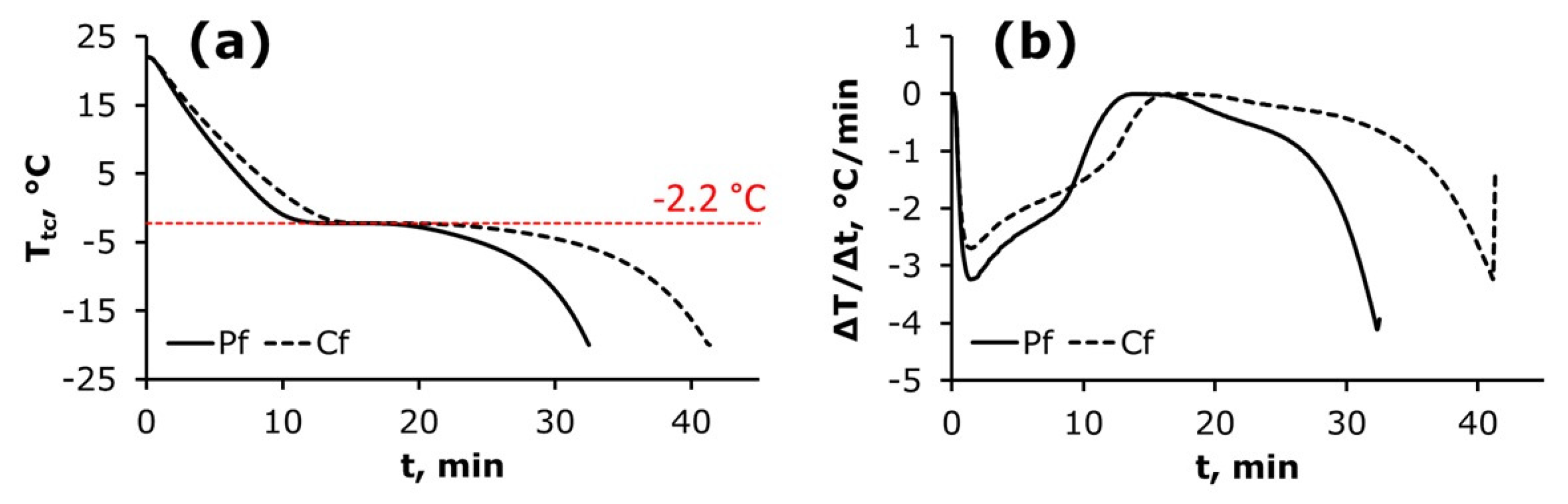
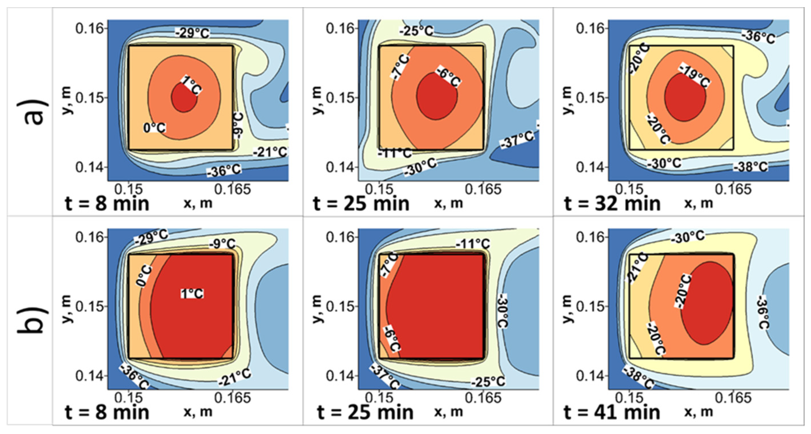
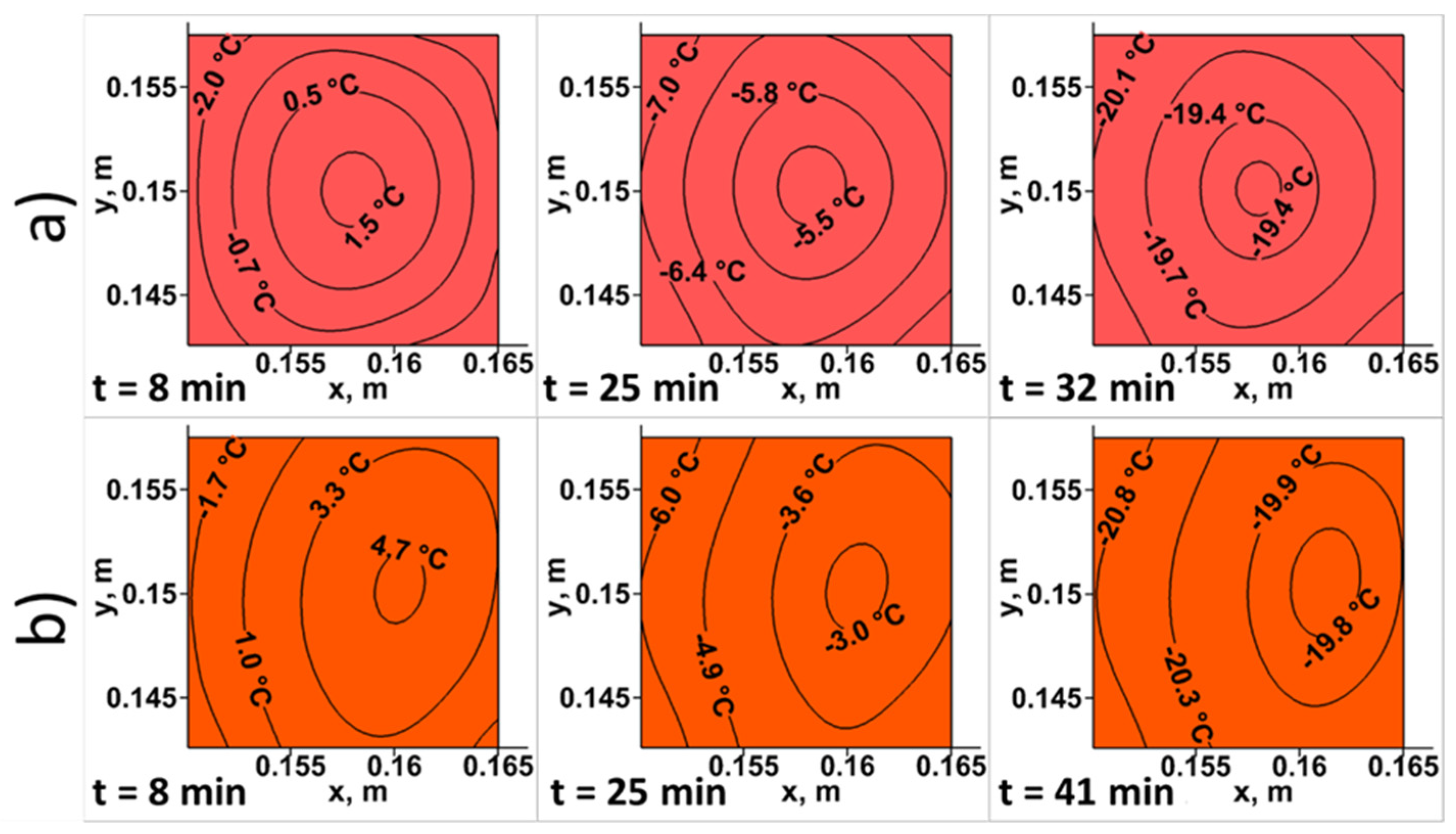
3.2. Effect of Pulsating Inlet Airflow on Heat Transfer

Figure 7 illustrates the changes in the thermal center temperature (hottest point) and the freezing rate of salmon for the two cases analyzed: pulsating and steady velocity inlet. The analysis of Figure 7a indicates that employing pulsating airflow at the inlet, as opposed to a steady velocity profile, led to a more expedited attainment of the target temperature of −20 °C for the salmon, resulting in a 21% reduction in processing time. During the cooling stage, the temperature of the food decreased linearly, with a freezing rate of 1.8 °C/min when pulsatile airflow was utilized, compared to 1.5 °C/min when steady airflow was employed at the inlet. In the phase change from liquid water to ice, the hottest point inside the food remained at the freezing temperature for 80 s with pulsed inlet airflow and 100 s with steady inlet airflow, necessitating an additional 25% of time. Figure 7b illustrates that the freezing rate increased rapidly when pulsating air flow was employed, reaching the target temperature faster than the case with steady airflow velocity inlet was imposed. Kono and colleagues [57] have quantitatively examined the interplay between freezing rate, ice crystal size, and color changes on the surface of salmon fillets. It was observed that quick freezing minimizes damage to the salmon tissue, enhances brightness, and imparts a whitish appearance. This suggests that using pulsating airflow leads to improved food quality during freezing. Furthermore, a reduction in process time translates to increased efficiency and productivity.
The temperature contours in Figure 8 illustrate the freezing process of a piece of salmon using pulsating or continuous airflow at the inlet, depicting three stages: cooling, phase change, and subcooling. The isotherms reveal that employing inlet pulsating airflow resulted in a more homogeneous salmon freezing than continuous airflow. This is attributed to the periodic disturbance of the boundary layer around the food, which enhanced the convective heat flow from the air to the food. Additionally, when the velocity was reduced due to the sinusoidal function, natural convection dominated around the food, altering the thermal boundary layer, as shown in Figure 8a at t = 1500 s. Figure 8b demonstrates that the boundary layer around the object remained constant while the front layer exhibited the most negligible thickness in the freezing process involving continuous inlet airflow.
Consequently, the higher temperature gradient resulted in a greater heat flux on that face, promoting a faster cooling rate from the front to the back of the food. In an investigation performed by Cui et al. [30], heat transfer and temperature distributions within the compartments and walls of a household refrigerator were examined. The researchers observed a significant phenomenon wherein localized airflow acceleration augmented heat exchange, particularly in areas with obstructions or near the air inlets, resulting in notable airflow disturbance. These findings underscore the advantageous impact of pulsating airflow in perturbing the air surrounding food items.
Figure 9a shows that when freezing is performed with pulsating airflow, the hottest point, known as the thermal center, aligns with the geometric center. This is different from freezing with continuous airflow at the entrance, where the thermal center is situated toward the rear face of the food. As a result, using pulsating airflow leads to a more even freezing process, with the most significant temperature difference occurring between the center and any of the surfaces of the piece of salmon. Upon analyzing the maximum temperature gradients within the food, as depicted in Figure 9a,b, it is evident that the temperature variance decreased from 3.5 °C at t = 8 min to 1.5 °C after 25 min and further to 0.7 °C at t = 32 min due to the pulsating airflow. Conversely, a maximum temperature difference of 1 °C was observed at t = 41 min with steady airflow. The pulsatile inlet airflow led to a 22% reduction in the overall freezing process compared to the constant velocity airflow. A prior study examining water freezing within a modified air tunnel featuring baffles observed comparable findings regarding freezing progression within the container. Similarly to the present findings, the baffles produced a perturbated airflow surrounding the object, resulting in faster and uniform freezing [8]. In food freezing, the main goal is to convert, in the quickest way, as much liquid water as possible into ice to prevent spoilage by microorganisms [58].
Figure 10 illustrates the progression of iso-concentration lines representing the available liquid water. Initially, the liquid water comprises 76% of the salmon’s weight. Following 8 min of cooling using continuous airflow, a substantial portion of the salmon’s water content remained in the liquid phase. However, pulsating airflow resulted in only the central region of the salmon exhibiting a liquid water concentration at the outset. At the same time, the edges experienced homogeneous freezing with a 30% liquid water concentration. After 25 min, the central region of the salmon exhibited a 20% liquid water content when subjected to pulsating airflow at the tunnel inlet, with the edges displaying a 16% liquid water content.
On the other hand, in the case with steady airflow, at t = 25 min, the center of the salmon had a liquid water content of 40%, with the upper, lower, and rear edges exhibiting a fluid range of 20%. However, the food’s front surface had the highest freezing rate. At the end of freezing, 9% of the weight of the salmon was liquid water, which was reached 10 min earlier by freezing with pulsating airflow, with a more homogeneous freezing rate and temperature distribution. The investigation into the movement of the liquid–solid front during the phase change revealed that the pulsating airflow at the entrance of the refrigeration tunnel led to a more uniform freezing distribution in the salmon, potentially improving the tissue quality of the food. A study was conducted on a convective process involving stationary air flow, focusing on the freezing of salmon in a natural convection freezing chamber [28]. The study observed that the heat transfer rate from food surfaces exposed to areas where air flowed faster was higher than that of other surfaces. This phenomenon is similar to a forced convection tunnel without pulsating airflow, where cooling occurs on the front surface directly exposed to the cold airflow. González et al. developed a numerical investigation to analyze the freezing process within a domestic freezer cabinet dominated by natural convection [21]. The findings revealed that situating the food directly with the freezer walls and heat exchangers could expedite the freezing rate. However, relocating the food to the central area of the chamber, where it is subjected to the rotational movement of cold air, can engender a more uniform freezing process and a reduced freezing rate. These discoveries were juxtaposed with the convective freezing process of consistent inlet airflow. It was noted that regions directly exposed to airflow fluctuations exhibit the most pronounced heat transfer rates. This phenomenon was also discernible in the freezing tunnel, even without pulsating inlet airflow.

3.3. Dimensionless Heat Flux Analysis and Energy Saving

An energy analysis was conducted to assess heat transfer using the Nusselt number, which characterizes heat transfer on each surface of the salmon piece. The Nusselt number distribution, illustrated in Figure 11, demonstrates that the front face experiences higher heat flux than the other surfaces, particularly during the cooling (8 min) and subcooling stages (32 min), as delineated in Table 3. It was noted that pulsating airflow resulted in elevated Nusselt values compared to continuous airflow, especially at t = 25 min when the Nusselt value on the front face was lower than on the other faces, contributing to the uniformity of salmon freezing. As presented in Table 3, the disparity in the values of the local Nu between the front and rear surfaces of the food is fourfold, alternating. In contrast, the ratio between the parallel horizontal surfaces is half the maximum value. A study by Mikheev et al. [13] experimentally demonstrated that pulsating forced flow can facilitate heat transfer from a cylinder in crossflow. The most significant improvement in average heat transfer occurred when two symmetric vortices were shed from opposite sides of the cylinder during one period of free-stream pulsations. The airflow patterns around the salmon induce fluctuations in the average heat flux. Freezing under a constant air velocity inlet reduces the magnitude of fluctuation, yielding an average Nusselt number ranging from 6 to 6.4. Conversely, freezing with a pulsating inlet airflow leads to Nusselt number values fluctuating between 7 and 9. This effect explains the faster freezing rate in the context of pulsating airflow freezing.
The overall energy consumption associated with freezing food in a tunnel is influenced by various factors, including the energy required for fan operation, heat generated during thawing, heat loss due to inadequate insulation, heat release during product replacement, and the primary objective of reducing food temperature. In this context, the thermal load of the product serves as a dependable indicator of the energy consumed during the food freezing process, typically constituting 50–80% of the total energy consumption [8]. Our analysis, along with equation 12, has indicated a heat rate of 33.5 W for continuous airflow and 42.6 W for pulsating airflow extracted from the food. That suggests a 21% increase in heat extraction from the food when using pulsating airflow for the same processing time, translating to substantial energy savings of equivalent magnitude.

4. Conclusions

Fluid mechanics and convective heat transfer in airflow inside a cooling tunnel along heat diffusion with liquid-to-solid phase change of water content inside a piece of salmon were described by conjugate mathematical modeling. The variation in food properties with temperature and the apparent constant pressure-specific heat that included the latent heat in the liquid–solid phase of water was incorporated into the governing equations. A novel pressure-correction iterative algorithm implemented in the finite volume method allowed a fast-accurate solution to the solid food freezing problem. Examining energy transfer during the convective freezing of salmon in a refrigeration tunnel, based on the results obtained by the computational model, yielded significant findings. The utilization of pulsating airflow, as opposed to steady inlet flow, resulted in a noteworthy 21% decrease in energy consumption and freezing time while concurrently enhancing the freezing rate. This improvement is advantageous in yielding smaller ice crystals and elevating food quality.
Furthermore, pulsating airflow facilitated a more even temperature distribution within the salmon, with a minimal 0.7 °C differential between the core and outer surfaces, compared to the 1 °C observed with continuous airflow. Additionally, the adoption of pulsating airflow led to elevated Nusselt values on the feed surfaces, ranging from 7 to 9, compared to 6 to 6.4 with continuous airflow. These outcomes underscore the potential of pulsating airflow technology to enhance energy efficiency in food freezing procedures, constituting a noteworthy advancement in this high-energy consumption application. The practical implications of the study are quality improvements in salmon, such as color and texture, should be estimated by predicting the freezing rate; the proposed computational model can calculate increments in frozen food production. Directions for future investigations should include three-dimensional analysis, the real shape of salmon pieces, turbulent conjugate convective freezing, an ensemble of salmon pieces, and exergy analysis to improve the freezing tunnel design.

Author Contributions

Conceptualization, R.L.-M. and L.P.; Writing—original draft, E.J.T., R.L.-M. and N.O.M.; Writing—review & editing, E.J.T.; Visualization, L.P.; Supervision, R.L.-M. and N.O.M. All authors have read and agreed to the published version of the manuscript.

Funding

This work was supported by the Research and Development National Agency, ANID-Chile, FONDECYT POSTDOCTORADO grant No. 3220297, FONDECYT grant No. 1200572, and FONDECYT grant No. 1231528.

Data Availability Statement

The original contributions presented in the study are included in the article, further inquiries can be directed to the corresponding author.

Conflicts of Interest

The authors declare no conflict of interest.

Nomenclature

AAmplitudeDimensionless
BCharacteristic length; square sidem
CLLift coefficientDimensionless
CLV, CLPLift coefficients due to viscous and pressure forcesDimensionless
CDDrag coefficientDimensionless
CDV, CDPDrag coefficients due to viscous and pressure forcesDimensionless
cpSpecific heat at constant pressureJ kg−1 K−1
CfContinuous flowDimensionless
fFrequencyHz
GrGrashoff numberDimensionless
gGravity constant m s−2
HHeight of tunnelm
kThermal conductivity W m−1K−1
L o Water Latent heat of fusion = 333.55kJ kg−1
LDDistance from the channel outlet to the downstream face of foodm
LUDistance from the channel inlet to upstream face of foodm
m f o o d Mass of foodkg
NuNusselt numberDimensionless
pPressurePa
PfPulsating flowDimensionless
PrPrandtl numberDimensionless
ReReynolds numberDimensionless
RiRichardson numberDimensionless
StStrouhal numberDimensionless
tTimes
t p r o c e s s Process times
TTemperature°C, K
uVelocity componentsm s−1
UInlet velocitym s−1
VmagVelocity magnitudem s−1
xPosition component m
x*Dimensionless coordinate around square foodDimensionless
XFraction Dimensionless
Greek letters
α Sub-relaxationDimensionless
βThermal expansion coefficientK−1
ε Convergence criteriaDimensionless
μ Dynamic viscosityPa s
ρ densitykg m−3
ϕ Generalized dependent variable
Subscripts
Free stream
avAverage
apApparent
bBottom
bwBond water
cfChange phase
fFront
finFinal
fluFluid
froFrozen
iHorizontal direction index; i-th term formula
iceQuantity of ice
inInlet
iniInitial
intInterface
jVertical direction index
mMean value
pPulsating
p0Natural frequency
rRear
refReference value
sQuantity of solids
solSolid
tTop
tcThermal center
uUnfrozen
uwUnfrozen water
wLiquid water
woInitial quantity of water
Superscript
kk-th term formula
ν Specific volume

References

  1. Liu, Z.; Lu, D.; Shen, T.; Guo, H.; Bai, Y.; Wang, L.; Gong, M. New configurations of absorption heat transformer and refrigeration combined system for low-temperature cooling driven by low-grade heat. Appl. Therm. Eng. 2023, 228, 120567. [Google Scholar] [CrossRef]
  2. Daghooghi-Mobarakeh, H.; Subramanian, V.; Phelan, P.E. Experimental study of water freezing process improvement using ultrasound. Appl. Therm. Eng. 2022, 202, 117827. [Google Scholar] [CrossRef]
  3. Sharif, Z.; Mustapha, F.; Jai, J.; Yusof, N.M.; Zaki, N. Review on methods for preservation and natural preservatives for extending the food longevity. Chem. Eng. Res. Bull. 2017, 19, 145. [Google Scholar] [CrossRef]
  4. Liu, Z.; Lou, F.; Qi, X.; Wang, Q.; Zhao, B.; Yan, J.; Shen, Y. Experimental study on cold storage phase-change materials and quick-freezing plate in household refrigerators. J. Food Process. Eng. 2019, 42, e13279. [Google Scholar] [CrossRef]
  5. Svendsen, E.S.; Widell, K.N.; Tveit, G.M.; Nordtvedt, T.S.; Uglem, S.; Standal, I.; Greiff, K. Industrial methods of freezing, thawing and subsequent chilled storage of whitefish. J. Food Eng. 2022, 315, 110803. [Google Scholar] [CrossRef]
  6. Yang, D.; Xie, J.; Tang, W.; Wang, J.; Shu, Z. Air-impingement freezing of peeled shrimp: Analysis of flow field, heat transfer, and freezing time. Adv. Mech. Eng. 2019, 11, 1687814019835040. [Google Scholar] [CrossRef]
  7. Alam, T.; Kim, M.H. A comprehensive review on single phase heat transfer enhancement techniques in heat exchanger applications. Renew. Sustain. Energy Rev. 2018, 81, 813–839. [Google Scholar] [CrossRef]
  8. Tabilo, E.J.; Moraga, N.O. Improved water freezing with baffles attached to a freezing tunnel: Mathematical modeling and numerical simulation by a conjugate finite volume model. Int. J. Refrig. 2021, 128, 177–185. [Google Scholar] [CrossRef]
  9. Kurtulmuş, N.; Sahin, B. Experimental investigation of pulsating flow structures and heat transfer characteristics in sinusoidal channels. Int. J. Mech. Sci. 2020, 167, 105268. [Google Scholar] [CrossRef]
  10. Ye, Q.; Zhang, Y.; Wei, J. A comprehensive review of pulsating flow on heat transfer enhancement. Appl. Therm. Eng. 2021, 196, 117275. [Google Scholar] [CrossRef]
  11. Blythman, R.; Persoons, T.; Jeffers, N.; Murray, D.B. Heat transfer of laminar pulsating flow in a rectangular channel. Int. J. Heat Mass Transf. 2019, 128, 279–289. [Google Scholar] [CrossRef]
  12. Akdag, U.; Akcay, S.; Demiral, D. Heat transfer enhancement with nanofluids under laminar pulsating flow in a trapezoidal-corrugated channel. Prog. Comput. Fluid Dyn. 2017, 17, 302–312. [Google Scholar] [CrossRef]
  13. Mikheev, N.I.; Molochnikov, V.M.; Mikheev, A.N.; Dushina, O.A. Hydrodynamics and heat transfer of pulsating flow around a cylinder. Int. J. Heat Mass Transf. 2017, 109, 254–265. [Google Scholar] [CrossRef]
  14. Saxena, A.; Ng, E.Y.K. Steady and pulsating flow past a heated rectangular cylinder(s) in a channel. J. Thermophys. Heat Trans. 2018, 32, 401–413. [Google Scholar] [CrossRef]
  15. Bhalla, N.; Dhiman, A.K. Pulsating flow and heat transfer analysis around a heated semi-circular cylinder at low and moderate Reynolds numbers. J. Braz. Soc. Mech. Sci. Eng. 2017, 39, 3019–3037. [Google Scholar] [CrossRef]
  16. Bayomy, A.M.; Saghir, M.Z. Heat development and comparison between the steady and pulsating flows through aluminum foam heat sink. J. Therm. Sci. Eng. Appl. 2017, 9, 031006. [Google Scholar] [CrossRef]
  17. Esfe, M.H.; Bahiraei, M.; Torabi, A.; Valadkhani, M. A critical review on pulsating flow in conventional fluids and nanofluids: Thermo-hydraulic characteristics. Int. Commun. Heat Mass Transf. 2021, 120, 104859. [Google Scholar] [CrossRef]
  18. Yang, B.; Gao, T.; Gong, J.; Li, J. Numerical investigation on flow and heat transfer of pulsating flow in various ribbed channels. Appl. Therm. Eng. 2018, 145, 576–589. [Google Scholar] [CrossRef]
  19. Hayakawa, S.; Fukue, T.; Sugimoto, Y.; Hiratsuka, W.; Shirakawa, H.; Koito, Y. Effect of rib height on heat transfer enhancement by combination of a rib and pulsating Flow. Front. Heat Mass Transf. 2022, 18, 1–9. [Google Scholar] [CrossRef]
  20. Moraga, N.O.; Rivera, D.R. Advantages in predicting conjugate freezing of meat in a domestic freezer by CFD with turbulence k-ɛ 3D model and a local exergy destruction analysis. Int. J. Refrig. 2021, 126, 76–87. [Google Scholar] [CrossRef]
  21. González, N.P.; Moraga, N.O. Energy and exergy analysis of conjugate 3D unsteady heat conduction with solidification of water by turbulent buoyancy-driven freezing of solid food in air. Therm. Sci. Eng. Prog. 2023, 37, 101566. [Google Scholar] [CrossRef]
  22. Hoang, D.K.; Lovatt, S.J.; Olatunji, J.R.; Carson, J.K. Validated numerical model of heat transfer in the forced air freezing of bulk packed whole chickens. Int. J. Refrig. 2020, 118, 93–103. [Google Scholar] [CrossRef]
  23. Huo, Y.; Yang, D.; Xie, J.; Yang, Z. Simulation Analysis and Experimental Verification of Freezing Time of Tuna under Freezing Conditions. Fishes 2023, 8, 470. [Google Scholar] [CrossRef]
  24. Rivera, D.R.; Moraga, N.O. Turbulent mixed convection of air in a cavity with a heat-conducting inner solid: Effect of surface radiation and thermal diffusivity on heat transfer and exergy destruction. Int. J. Mech. Sci. 2022, 218, 107035. [Google Scholar] [CrossRef]
  25. Tabilo, E.J.; Moraga, N.O. Unsteady conjugate model of fluid mechanics and mass transfer for butanol pervaporation process by non-porous membrane. Int. Commun. Heat Mass Transf. 2021, 127, 105539. [Google Scholar] [CrossRef]
  26. Rodríguez-Ramos, F.; Tabilo, E.J.; Moraga, N.O. Modeling inactivation of Clostridium botulinum and vitamin destruction of non-Newtonian liquid-solid food mixtures by convective sterilization in cans. Innov. Food Sci. Emerg. Technol. 2021, 73, 102762. [Google Scholar] [CrossRef]
  27. Rodríguez-Núñez, K.; Tabilo, E.; Moraga, N.O. Conjugate unsteady natural heat convection of air and non-Newtonian fluid in thick-walled cylindrical enclosure partially filled with a porous media. Int. Commun. Heat Mass Transf. 2019, 108, 104304. [Google Scholar] [CrossRef]
  28. González, N.P.; Rivera, D.R.; Moraga, N.O. Conjugate turbulent natural heat convection and solid food freezing modelling: Effects of position and number of pieces of salmon on the cooling rate. Therm. Sci. Eng. Prog. 2021, 26, 101101. [Google Scholar] [CrossRef]
  29. Buceta, J.P.; Passot, S.; Scutellà, B.; Bourlés, E.; Fonseca, F.; Trelea, I.C. Use of 3D mathematical modelling to understand the heat transfer mechanisms during freeze-drying using high-throughput vials. Appl. Therm. Eng. 2022, 207, 118099. [Google Scholar] [CrossRef]
  30. Cui, P.; He, L.; Mo, X. Flow and heat transfer analysis of a domestic refrigerator with complex wall conditions. Appl. Therm. Eng. 2022, 209, 118306. [Google Scholar] [CrossRef]
  31. Gulati, T.; Datta, A.K. Enabling computer-aided food process engineering: Property estimation equations for transport phenomena-based models. J. Food Eng. 2013, 116, 483–504. [Google Scholar] [CrossRef]
  32. Rao, M.; Rizvi, S.; Datta, A.; Ahmed, J. Engineering Properties of Foods, 4th ed.; CRC Press, Taylor and Francis Group: Boca Raton, FL, USA, 2014. [Google Scholar]
  33. de Lima, W.C.P.B.; Nascimento, L.P.C.; Dantas, R.L.; Tresena, N.L.; Júnior, J.B.S.; de Lima, G.S.; de Lima, A.G.B. Heat Transfer in the Cooling, Freezing and Post-Freezing of Liquid Food: Modeling and Simulation. Diffus. Found. 2020, 25, 37–53. [Google Scholar] [CrossRef]
  34. Hoang, D.K.; Lovatt, S.J.; Olatunji, J.R.; Carson, J.K. Improved prediction of thermal properties of refrigerated foods. J. Food Eng. 2021, 297, 110485. [Google Scholar] [CrossRef]
  35. Yu, J.Y.; Lin, W.; Zheng, X.T. Effect on the flow and heat transfer characteristics for sinusoidal pulsating laminar flow in a heated square cylinder. Heat Mass Transf./Waerme Stoffuebertragung 2014, 50, 849–864. [Google Scholar] [CrossRef]
  36. Kiani, H.; Sun, D.W. Numerical simulation of heat transfer and phase change during freezing of potatoes with different shapes at the presence or absence of ultrasound irradiation. Heat Mass Transf. 2018, 54, 885–894. [Google Scholar] [CrossRef]
  37. Wang, W.; Li, W.; Bu, Y.; Li, X.; Zhu, W. Nano freezing–thawing of Atlantic salmon fillets: Impact on thermodynamic and quality characteristics. Foods 2023, 12, 2887. [Google Scholar] [CrossRef] [PubMed]
  38. Rivera, D.R.; Moraga, N.O. Energy analysis of convective freezer cabinet with PCMs and salmon-fillet during charging, discharging and normal operation processes by CFD modeling. J. Energy Storage 2024, 83, 110558. [Google Scholar] [CrossRef]
  39. ASHRAE. 2014 ASHRAE Handbook: Refrigeration; ASHRAE: Atlanta, GA, USA, 2014. [Google Scholar]
  40. Çengel, Y.A. Heat and Mass Transfer: A Practical Approach, 3rd ed.; McGraw-Hill Science/Engineering/Math: University Park, PA, USA, 2007; Available online: https://books.google.cl/books?id=WgZaAAAAYAAJ (accessed on 22 July 2011).
  41. Choi, Y.; Okos, M.R. Effects of temperature and composition on the thermal properties of foods. J. Food Process. Appl. 1986, 1, 93–101. [Google Scholar]
  42. Moraga, N.O.; Jaime, J.I.; Cabrales, R.C. An approach to accelerate the convergence of SIMPLER algorithm for convection-diffusion problems of fluid flow with heat transfer and phase change. Int. Commun. Heat Mass Transf. 2021, 129, 105715. [Google Scholar] [CrossRef]
  43. Li, Z.Y.; Tao, W.Q. A new stability-guaranteed second-order difference scheme. Numer. Heat Transf. Part B Fundam. 2002, 42, 349–365. [Google Scholar] [CrossRef]
  44. Patankar, S.V. Numerical Heat Transfer and Fluid Flow, 6th ed.; Hemisphere Publishing Corporation: Washington, DC, USA, 1980. [Google Scholar]
  45. Curtiss, C.F.; Hirschfelder, J.O. Integration of stiff equations. Proc. Natl. Acad. Sci. USA 1952, 38, 235–243. [Google Scholar] [CrossRef]
  46. Okajima A, Strouhal number of rectangular cylinders. J. Fluid Mech. 1982, 123, 379–398. [CrossRef]
  47. Fowler, T.S.; Witherden, F.D.; Girimaji, S.S. Pulsating flow past a square cylinder: Analysis of force coefficient spectra and vortex structure development. J. Fluids Eng. Trans. ASME 2020, 142, 121106. [Google Scholar] [CrossRef]
  48. Mahir, N.; Altaç, Z. Numerical investigation of flow and combined natural-forced convection from an isothermal square cylinder in cross flow. Int. J. Heat Fluid Flow 2019, 75, 103–121. [Google Scholar] [CrossRef]
  49. Luo, S.C.; Tong, X.H.; Khoo, B.C. Transition phenomena in the wake of a square cylinder. J. Fluids Struct. 2007, 23, 227–248. [Google Scholar] [CrossRef]
  50. Sharma, A.; Eswaran, V. Heat and fluid flow across a square cylinder in the two-dimensional laminar flow regime. Numer. Heat Transf. Part A Appl. 2004, 45, 247–269. [Google Scholar] [CrossRef]
  51. Saha, A.K.; Biswas, G.; Muralidhar, K. Three-dimensional study of flow past a square cylinder at low Reynolds numbers. Int. J. Heat Fluid Flow 2003, 24, 54–66. [Google Scholar] [CrossRef]
  52. Robichaux, J.; Balachandar, S.; Vanka, S.P. Three-dimensional Floquet instability of the wake of square cylinder. Phys. Fluids 1999, 11, 560–578. [Google Scholar] [CrossRef]
  53. Sohankar, A.; Norberg, C.; Davidson, L. Numerical simulation of unsteady low-Reynolds number flow around rectangular cylinders at incidence. J. Wind Eng. 1997, 69–71, 189–201. [Google Scholar] [CrossRef]
  54. Sen, S.; Mittal, S.; Biswas, G. Flow past a square cylinder at low Reynolds numbers. Int. J. Numer. Methods Fluids 2011, 67, 1160–1174. [Google Scholar] [CrossRef]
  55. Moschandreou, T.; Zamir, M. Heat transfer in a tube with pulsating flow and constant heat flux. Int. J. Heat Mass Transf. 1997, 40, 2461–2466. [Google Scholar] [CrossRef]
  56. Ji, T.H.; Kim, S.Y.; Hyun, J.M. Experiments on heat transfer enhancement from a heated square cylinder in a pulsating channel flow. Int. J. Heat Mass Transf. 2008, 51, 1130–1138. [Google Scholar] [CrossRef]
  57. Kono, S.; Kon, M.; Araki, T.; Sagara, Y. Effects of relationships among freezing rate, ice crystal size and color on surface color of frozen salmon fillet. J. Food Eng. 2017, 214, 158–165. [Google Scholar] [CrossRef]
  58. Li, D.; Zhu, Z.; Sun, D.W. Effects of freezing on cell structure of fresh cellular food materials: A review. Trends Food Sci. Technol. 2018, 75, 46–55. [Google Scholar] [CrossRef]
Figure 1. Physical model of salmon freezing by pulsating air flow in convective freezer tunnel.
Processes 12 01852 g001
Figure 2. (a) Mean Nusselt number for five grids; (b) Strouhal number for five time-step, and time of computation, when Re = 250.
Processes 12 01852 g002
Figure 3. Effects of the inlet: (a) pulsating amplitude, and (b) pulsating frequency, on the Nusselt number, Re = 250.
Processes 12 01852 g003
Figure 4. (a) Lift coefficient of continuous and pulsating flow; Peaks of vortex-shedding frequency of inlet (b) pulsating and (c) continuous flow, for Re = 250.
Processes 12 01852 g004
Figure 5. Evolution of streamlines around the square food for a cycle of vortex formation and shedding in continuous inlet airflow with Re = 250.
Processes 12 01852 g005
Figure 6. Evolution of streamlines around the square salmon piece for a cycle of vortex formation and shedding in pulsating inlet airflow with Re = 250.
Processes 12 01852 g006
Figure 7. Evolution of (a) thermal center temperature and (b) freezing rate by continuous and pulsating inlet air flow with Re = 250 to freeze a piece of salmon.
Processes 12 01852 g007
Figure 8. Isotherms of salmon freezing by (a) pulsating airflow and (b) continuous airflow in a refrigeration tunnel, Re = 250.
Processes 12 01852 g008
Figure 9. Evolution of isotherms in the salmon piece at three freezing stages by inlet: (a) pulsed and (b) continuous airflow with Re = 250.
Processes 12 01852 g009
Figure 10. History of the water fraction contours of salmon freezing by inlet: (a) pulsating and (b) continuous airflow when Re = 250.
Processes 12 01852 g010
Figure 11. Local distribution of the Nusselt number around the frozen salmon piece by inlet pulsed and continuous airflow with Re = 250.
Processes 12 01852 g011
Table 1. Assessment of Mesh Independence for Velocity Profiles at y = 10B and x = 10.5B.
ProfilesΔumaxΔvmax
G5-G1G5-G2G5-G3G5-G4G5-G1G5-G2G5-G3G5-G4
Horizontal
y = 10B
1.3 × 10−14.0 × 10−21.1 × 10−11.0 × 10−12.3 × 10−14.4 × 10−23.4 × 10−13.5 × 10−1
Vertical
x = 10.5B
6.4 × 10−26.2 × 10−26.4 × 10−25.5 × 10−22.2 × 10−21.3 × 10−21.4 × 10−21.3 × 10−2
Table 2. Effect of Reynolds number on Strouhal number, drag/lift coefficients, and Nusselt number for airflow around square solid inside refrigerator tunnel, 100 ≤ Re ≤ 250.
Forced ConvectionMix. Conv.
Reynolds Number100120140160200250(Ri = 0.65)
Strouhal number
Present0.1520.1550.1570.1550.1550.1470.151
Mahir and Altaç 3D, 2019 [48]0.1520.1580.1580.1640.1520.152
Okajima, 1982 (exp.) [46]0.1420.1450.1440.143
Luo et al., 2007 (exp.) [49]0.1450.1520.1590.159
Sharma and Eswaran, 2004 [50]0.1520.1590.1630.164
Saha et al., 2003 [51]0.1520.1590.1630.1590.160.164
Fowler et al., 2020 [47]0.153
Mean CD
Present1.4711.4071.4021.4041.3941.3441.53
Mahir and Altaç 3D, 2019 [48]1.4331.4431.4611.4831.4911.554
Okajima, 1982 (exp.) [46]1.5931.4761.479
Robichaux et al., 1999 [52]1.5331.5411.5611.5831.6361.671
Saha et al., 2003 [51]1.4961.5071.5581.5251.5951.682
Fowler et al., 2020 [47]1.484
RMS CL
Present0.1330.2000.2420.2830.3700.4730.660
Mahir and Altaç 3D, 2019 [48]0.1760.2260.2700.3180.3030.313
Sharma and Eswaran, 2004 [50]0.1920.2300.2700.317
Sohankar et al., 1997 [53]0.1530.367
Sen et al., 2011 [54]0.1910.2430.276
Fowler et al., 2020 [47]0.433
Mean Nu
Present4.0574.3994.7084.9835.4515.9476.453
Mahir and Altaç 3D, 2019 [48]4.0324.3554.6624.9425.2725.618
Mahir and Altaç 2D, 2019 [48]4.0204.3564.6574.9325.4356.02
Sharma and Eswaran, 2004 [50]4.0104.3754.694.983
Yu et al., 2014 [35]4.420
Table 3. Average Nusselt number on each side of the salmon slice for each freezing stage.
Mean Nut = 8 mint = 25 mint = 32 min/41 min
PulsatingContinuousPulsatingContinuousPulsatingContinuous
Front16.712.77.012.716.812.7
Bottom7.84.68.34.67.84.6
Rear4.54.412.05.04.64.3
Top8.05.05.24.78.04.6
Disclaimer/Publisher’s Note: The statements, opinions and data contained in all publications are solely those of the individual author(s) and contributor(s) and not of MDPI and/or the editor(s). MDPI and/or the editor(s) disclaim responsibility for any injury to people or property resulting from any ideas, methods, instructions or products referred to in the content.

