Study on Wind Farm Flow Field Characteristics Based on Boundary Condition Optimization of Complex Mountain Numerical Simulation

Abstract

The accurate prediction of the flow field characteristics of complex mountains is of great practical significance for the development and construction of wind farms, but it is not yet fully understood. The main purpose of this study is to propose a method for the study of flow field characteristics under complex mountain conditions, which can optimize the boundary conditions required for numerical simulation through the wind acceleration ratio and, at the same time, couple the numerical simulation and wind measurement data to reflect the real mountain flow field distribution. The results show that the proposed method has good applicability in complex mountain wind farms, can reproduce the real flow field distribution, and has a certain practical value. Wind speed distribution and turbulence intensity are greatly affected by boundary conditions such as wind speed and wind direction and are also affected by the shielding effect brought by terrain changes. The contrast between 120° and 150° wind direction is more obvious. When the incoming wind moves to the top of a mountain or the ridgeline, it will form a low-speed wake area behind it, resulting in reduced wind speed, increased turbulence intensity, and an unstable flow field.

1. Introduction

The use of non-renewable energy sources, such as coal and oil, has caused severe environmental pollution, leading to increasing global warming and greenhouse effects [1]. With the continuous growth in global energy demand and the increasing awareness of environmental protection, renewable energy generation, as an environmentally friendly and sustainable form of energy, has been receiving more and more attention. Wind energy, as a renewable energy source, is characterized by its large reserves, wide distribution, and high degree of commercialization, therefore, its important status in the energy sector is continuously being highlighted [2]. According to the Global Wind Energy Council’s “Global Wind Report 2023” in 2022, the global new wind power installed capacity was 77.6 GW, bringing the total wind power installed capacity to 906 GW. Additionally, by 2030, the development of the wind power industry in China is expected to maintain strong momentum, continuing to be the largest wind power market in the world [3]. Unlike the mostly flat terrains of Europe, over two-thirds of China’s land comprises complex terrains. Due to the acceleration effect of the terrain, wind speeds in complex terrains are often higher compared to that of flat terrains. Since wind power is proportional to the cube of the local wind speed, the increase in wind speed significantly enhances wind energy efficiency and output. As wind resources continue to be exploited, apart from offshore wind power, wind farm siting is gradually shifting towards complex terrains [4,5]. However, the intricate terrain and varying wind conditions present significant challenges and difficulties in understanding the flow field characteristics of wind farms in complex terrains. Therefore, it is essential to conduct research that accurately characterizes the wind flow in these complex terrains.

Generally speaking, the methods for studying the distribution characteristics of flow fields in complex terrains typically include field measurements, wind tunnel tests, and numerical simulations. Field measurements can obtain real data of local environmental characteristics and are the most direct and effective method [6,7,8]. However, they can only measure limited points, lacking representativeness in complex terrains. Wind tunnel experiments are conducted indoors, with minimal influence from climatic conditions and time, allowing for accurate control of experimental conditions [9,10]. Nevertheless, they must adhere to similarity theory and scaling, which limits the spatial range. Computational fluid dynamics (CFD) simulations using complex nonlinear models can provide full flow field data at all positions within the computational domain. With the rapid advancement of computer technology, CFD has become a highly efficient, low-cost, and energy-saving method for simulating flow fields in complex terrains. In terms of turbulence simulation, the Reynolds-averaged Navier–Stokes (RANS) model can accurately simulate the mean wind field through the control equations of averaged fluid motion [11]. Castro [12] applied the RANS method to the numerical simulation of the wind field over Askervein hill. A comparison with measured data showed that the RANS method is reliable for mean wind fields. Paiva [13] conducted numerical simulations of atmospheric boundary layer flow over an isolated vegetated hill based on the RANS method. The numerical results indicated that the method’s calculated vertical distribution of mean velocity and acceleration ratio is reasonable. Dhunny [14] performed a series of three-dimensional steady-state RANS simulations for the real terrain of Mauritius, analyzing the wind speed distribution characteristics. The results showed that the geographical distribution of seasonal wind speeds is strongly influenced by local topography. Although the large eddy simulation (LES) model can provide time-varying flow characteristics [15,16], it requires extremely high computational resources and long simulation times, making it unsuitable for assessing the mean wind field in complex terrains.

When applying the RANS model to calculate the flow field distribution in complex terrains, inlet boundary conditions such as mean wind speed, wind direction, and wind profile are crucial factors affecting the accuracy of the results [17,18]. To address the issue of poorly defined boundary conditions due to the limited number of meteorological towers or their placement far from the inlet boundary, many researchers use mesoscale numerical simulations to obtain these conditions [19,20]. However, mesoscale simulations are based on global numerical weather prediction (NWP) models. The resolution of NWP may be lower than that of local wind field data, potentially leading to the accumulation of downscaling errors. Therefore, it remains necessary to use measured data to provide boundary information for RANS simulations to achieve more accurate flow field distributions. Song [21] established a rough relationship between boundary wind speeds and those measured with meteorological towers, and, based on this, they implemented feedback processing to search for boundary wind speeds that match those measured with the towers. Yan and Li [22] combined single meteorological tower measurements with RANS simulations to predict wind speeds at each site within a wind farm, reproducing the spatial variability of wind speeds characteristic of complex terrains. Tang [23] integrated multiple wind speed measurements and RANS simulations for wind energy resource assessment in complex terrains, achieving accurate wind speed estimations. Cheng [18] proposed a data fusion method based on vertical multi-point wind speed (including wind direction) measurements and RANS simulation data, creating a polar coordinate diagram that simultaneously represents wind direction and wind profile index. These studies adopted iterative methods to adjust the inlet boundary conditions until the corresponding values in the database were matched. Although effective, this matching process converges slowly and typically requires more computational resources.

In the process of modeling terrain for the numerical simulation of flow fields in complex terrains, directly truncating digital terrain boundaries due to the undulating mountainous terrain and research scope limitations may cause elevation discontinuities, forming “artificial cliffs”. This can significantly hinder the incoming wind at the model’s edges, leading to flow separation and unrealistic airflow. To avoid this issue, many researchers have considered various forms of transition sections. Maurizi [24] used a boundary transition slope (BTS) with a maximum gradient of 10% to connect the wind tunnel floor with the top of the complex terrain model, allowing the incoming wind to transition smoothly into the study area. Hu [25] derived a theoretical curve based on flow theory around a cylinder and compared the flow transition performance of this theoretical curve with that of a traditional slope transition in a wind tunnel. The results indicated that the theoretical curve provided a better flow transition performance. Ren [26] considered the compatibility between the development of the mean wind speed profile and a cosine-squared hill function during terrain modeling, thus using a cosine-squared curve to smooth the terrain boundary. Huang [27] determined a new easing curve derived from the Witoszynski curve and validated its applicability in three-dimensional wind field numerical simulations of deep-cut valleys based on measured data. Although these transition curves allow the incoming wind to transition smoothly onto the study terrain, the variations in curve forms are limited and ignore the original terrain changes within the transition section, deviating from the actual conditions.

This paper proposes a new method that optimizes the numerical simulation boundary conditions through the wind speed acceleration ratio, improving the accuracy of flow field reproduction. It also couples numerical simulations with wind measurement data to reconstruct the mean flow field distribution in complex terrains. This study aims to address the practical significance of accurately predicting flow field characteristics in complex mountainous terrains, which is crucial for the development and construction of wind farms.

The first part of this paper is the introduction. The method will be introduced in the second part. The third part applies the proposed method to a real case study with complex terrain conditions. The fourth part analyzes the numerical simulation results, and the fifth part summarizes the conclusions of this paper.

2. Methodology

Given the existing issues in the numerical simulation of complex terrains, let us assume that there is a meteorological tower within the study area of the wind farm. The process of the method is illustrated in Figure 1 and will be discussed in the following steps:

(A) Wind data

Collect meteorological tower data for at least one year to analyze local meteorological characteristics. After calibration, filtering, and correction, obtain wind rose charts showing wind speed distribution and turbulence intensity, focusing on the mean wind speed for each wind direction. The wind speed and direction data at 70 m from the meteorological tower are taken as the focus of this study and are used to generate the initial boundary conditions for CFD simulations and for the correction and comparison of simulation results.

(B) Terrain Modeling

Select a meteorological tower with good wind measurement data and its surrounding area as the study region to obtain complex terrain data that include the study area. Under complex terrain conditions, if the influence of multiple wind directions on the flow field is to be considered, it is preferable to crop the study area into a circular shape to better achieve wind direction conversion. To preserve the flow field distribution of the transition section and ensure that the numerical simulation results more accurately reflect the characteristics of the actual terrain flow field, it is necessary to add transition sections according to Equation (1) [28], allowing the incoming wind to transition smoothly to the same elevation at the terrain edge. This method ensures that the simulated flow fields are consistent with the real terrain’s wind conditions, improving the overall accuracy and reliability of the numerical simulation.

$$z_n\left(x,y\right)=\left\{\begin{array}{ll}0& N+R<\sqrt{\left(x^2+y^2\right)}\\ z_e\left(x,y\right)\cdot \left[1-{\displaystyle \frac{\left(\sqrt{\left(x^2+y^2\right)}-R\right)}{N}}\right]& R<\sqrt{\left(x^2+y^2\right)}\le N+R\\ z_e\left(x,y\right)& 0\le \sqrt{\left(x^2+y^2\right)}\le R\end{array}\right.$$

(1)

where $z_n\left(x,y\right)$ represents the adjusted terrain elevation (m); $z_e\left(x,y\right)$ denotes the original terrain coordinate point elevation (m); $R$ is the radius of the actual terrain to be preserved, that is, the horizontal distance from the boundary point of the original terrain to the center of the study area (m); and $N$ is the length of the transition section (m).

To obtain results for multiple wind directions, the traditional rectangular fluid domain achieves changes in wind direction by rotating the internal terrain model [11,29]. However, this requires re-meshing for each change in wind direction, introducing a certain amount of grid error. The RANS model in numerical simulations can be used to simulate the flow field of complex terrains with at least 12 wind directions (typically evenly distributed over 360°, with each wind direction at 30° intervals). By controlling the terrain model at the center and establishing a cylindrical fluid domain outside, the fluid domain sides can be evenly divided into multiple sections according to the total number of studied directions. For the current operating condition’s wind direction, one side is designated as the inlet and the other side as the outlet. When changing the wind direction, the cylindrical fluid domain only requires renaming the inlet and outlet to achieve wind direction adjustment, thus avoiding the generation of grid errors.

(C) Boundary Condition Optimization

Regarding the optimization of boundary conditions in numerical simulations, this paper first conducts an initial numerical simulation based on the wind profile at the meteorological tower location for a specific wind direction. The wind profile index corresponding to each wind direction interval in the measurement data can be used to obtain the average wind speed value with the highest probability of occurrence. According to the power law defined in China’s “Load Code for the Design of Building Structures” [30], the wind profile can be fitted as shown in Equation (2). The accelerated change in the wind profile after passing through the complex terrain is shown in Figure 2. After obtaining the initial flow field data, the wind speed acceleration ratio at a certain height of the meteorological tower is calculated. The acceleration ratio is defined as the ratio of the average wind speed over the terrain to the average wind speed at the same height over flat terrain, where the height refers to the relative height above the ground. The wind acceleration ratio obtained from the initial numerical simulation is shown in Equation (3). The inlet wind speed is corrected using the acceleration ratio with the calculation formula shown in Equation (4). Conducting a second numerical simulation with the corrected wind speed will yield a flow field distribution that is closer to that of the actual conditions.

The wind profile from the first numerical simulation is as follows:

$$U_0(z)=U_{10}({\displaystyle \frac{z}{10}}{)}^{\mathsf{\alpha }}$$

(2)

where $U_0(z)$ represents the average wind speed (m/s) at a certain height z at the meteorological mast;$U_{10}$ is the wind speed 10 m (m/s) above the ground obtained from the analysis of wind measurement data; $\mathsf{\alpha }$ is the ground roughness index, depending on the site conditions; and $z$ represents the coordinate value at the same height (m).

The wind acceleration ratio ($R\left(z\right)$) is as follows:

$$R\left(z\right)={\displaystyle \frac{U}{U_1(z)}}$$

(3)

where $U$ represents the average wind speed (m/s) at a certain height above the ground in the wind measurement data and $U_1(z)$ represents the average wind speed (m/s) at the same height as $U$ in the first numerical simulation.

The wind profile of the second numerical simulation is as follows:

$$U_2(z)={\displaystyle \frac{U_1(z)}{R\left(z\right)}}$$

(4)

where $U_2(z)$ is the inlet velocity (m/s) of the second numerical simulation.

(D) Results Analysis

Following these steps, flow field data for the wind farm under various wind directions can be obtained. By extracting and comparing flow field data from different locations, wind directions, and heights, we can perform a comprehensive analysis of the data. Considering that the distribution of average wind speed can, to a certain extent, reflect the quality of wind resources, it is one of the main parameters in the study of flow field characteristics. Meanwhile, turbulence intensity directly affects the stability and distribution of flow field characteristics and is primarily divided into incoming turbulence intensity and characteristic turbulence intensity, which are significantly influenced by terrain effects [31]. This paper mainly selects these two parameters to analyze the flow field characteristics in complex terrains. In numerical simulations, the calculation formula for turbulence intensity ($TI$) is as follows:

$$TI={\displaystyle \frac{\sqrt{2k/3}}{U_z}}$$

(5)

where $U_z$ represents the wind speed value at height $z$ in the numerical simulation and $k$ is the turbulence kinetic energy (m²/s²).

3. Case Analysis of Wind Farms in Complex Terrains

3.1. Introduction to the Wind Farm

To illustrate the feasibility of the proposed method, the Jǐnpíng Xī Wind Farm in Yunnan Province, China, is taken as an example. The wind farm is located in Qiūběi County, Wenshan Prefecture, Yunnan Province, with geographical coordinates between 23°51′ to 24°18′ N latitude and 103°38′ to 103°59′ E longitude, at an altitude of 1900 m to 2350 m. This wind farm is situated in a low-latitude plateau with a significant monsoon climate and a three-dimensional climate. Its wind energy resources have a complex spatiotemporal distribution, and the terrain and topography are complex and variable, making it a typical mountainous wind farm.

3.2. On-Site Measurement and Wind Data Processing

Due to the extensive coverage area of the wind farm site, the distribution of anemometer towers is relatively scattered. However, from the perspective of the number and distribution of anemometer towers, measurement height, measurement period, and data quality, the existing anemometer towers provide good control over the site area. To study the distribution pattern of the flow field characteristics under complex mountainous conditions, a representative anemometer tower T was selected, located at 24°4′38.58′′ N latitude, 103°45′3.24′′ E longitude at an altitude of 2204 m. The wind measurement period started from 8 June 2012 to 28 February 2014, covering a full year of measurement. The equipment used is the Spanish KINTECH wind measurement instrument, with the anemometer sensor measuring wind speeds ranging from 1 m/s to 96 m/s, with a slope factor of 0.765 m/s/Hz. The wind vane measures the wind direction within a range of 0 to 360°, with an accuracy of 0.25% (1°). Data sampling is carried out every 10 min, obtaining the 10-min average wind speed and 10-min average wind direction. The wind speed levels are 10 m, 30 m, 50 m, and 70 m, and the wind direction levels are 10 m and 70 m.

The wind rose chart showing wind speed and turbulence intensity for 12 wind directions is illustrated in Figure 3. It can be observed that the predominant wind direction is clearly concentrated in the W sector, accounting for 23.59% of the frequency, followed by the WSW and SSE sectors, with frequencies of 19.05% and 12.77%, respectively. Most wind speeds vary within the range of 5 m/s to 10 m/s. Notably, the average wind speed in the WSW sector is 7.99 m/s, which is slightly higher than the average wind speed of 7.56 m/s in the dominant W sector. The turbulence intensity is mainly concentrated between 0.1 and 0.3, generally indicating a medium to low turbulence intensity.

3.3. Numerical Simulation

3.3.1. Geometric Model and Computational Domain

High-resolution remote sensing elevation data with a resolution of 12.5 m were downloaded from the Alaska Satellite Facility (NASA Synthetic Aperture Radar data) website. The research area was set with the wind measurement tower T as the center with a radius of 1500 m, as shown in Figure 4a. The study area contains three ridgelines in different directions and features peaks and valleys, representing the characteristics of a complex mountainous terrain. The parameters for the transition section were selected as R = 1500 m and N = 1000 m, as shown in Figure 4b.

This study utilizes Rhino 6 modeling software to construct the terrain model and computational domain. The computational domain has a circular base with a radius of 5000 m, centered at the location of the meteorological mast T, at a height of 5000 m, ensuring that the blockage ratio does not exceed 3% [32]. The entire fluid domain is divided into the following three parts: the inner terrain region, the middle transition section, and the outer region, as shown in Figure 5.

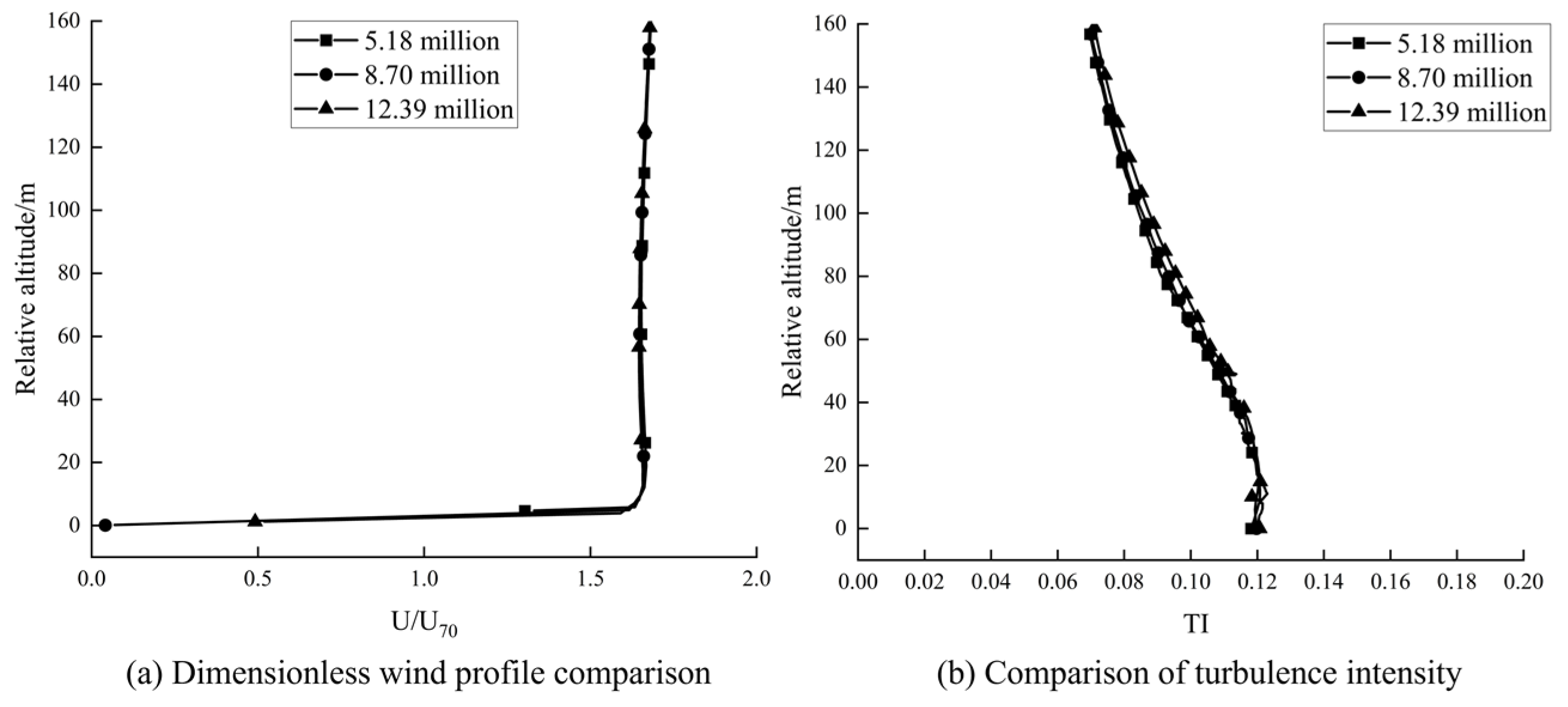
3.3.2. Mesh Division and Mesh Independence

Considering the complexity of the terrain and the surface of the transition section, a mixed division method of tetrahedral and hexahedral meshes is adopted. Near the ground surface, hexahedral meshes are used, while tetrahedral meshes are primarily used above the terrain. Mesh refinement is implemented using the Body of Influence (BOI) method. This approach allows for the refinement and control of the mesh quantity over the entire domain and above the terrain without dividing the computational domain. In the horizontal direction, the mesh size distribution is consistent with the fluid domain distribution. The largest mesh sizes are in the outer regions, decreasing progressively from the outside to the inside, with the smallest mesh sizes being above the terrain. Vertically, to capture the flow details above the ground with the finer mesh sizes, boundary layer meshes are set near the ground surface. The mesh growth rate is 1.08, with 10 layers of meshes, and the height of the first boundary layer is determined by the mesh-independent solution. Additionally, the mesh size is controlled to increase progressively from the bottom to the top, as illustrated in Figure 6.

By controlling the grid size, three different mesh quantities were obtained for grid independence verification, namely 5.18 million, 8.70 million, and 12.39 million grids. Numerical simulations were conducted on these three mesh models under a 270° incoming wind direction (W wind direction), comparing the dimensionless wind speed profile and the turbulence intensity at a height of 70 m from the wind measurement tower. The wind speed at the entrance at a height of 70 m is defined as U₇₀ (m/s), and U is the wind speed at different heights above the terrain at the location of the wind measurement tower (m/s). As shown in Figure 7, the results indicate that the wind profiles and turbulence intensities of the three different mesh quantities almost completely overlap. To ensure computational accuracy and save computational resources, this study selects the 8.70 million grid model for the numerical simulations of complex terrain. Under this grid size control, the height of the first boundary layer is 5 m.

3.3.3. Boundary Conditions and Operating Conditions

The top of the computational domain is set with symmetric boundary conditions, and one half of the sides is set as the velocity inlet, while the other half is designated as the pressure outlet. The specific range varies with the computational operating conditions. The bottom terrain and transition section are set as walls, employing no-slip boundary conditions. Wall functions are used to convert the roughness length of the complex terrain surface into physical roughness height, determined according to Equation (6) [33,34].

$$k_s={\displaystyle \frac{9.793z_0}{C_s}}$$

(6)

where $k_s$ represents the physical height of the roughness; $C_s$ is the roughness constant, taken as 0.5; and $z_0$ is the roughness length, set to 0.03.

The inlet of the computational domain is compiled using a user-defined function (UDF) based on load specifications to define the incoming wind profile and turbulence intensity [30]. The type of wind field, description, surface roughness index α, and gradient wind height $z_{\mathrm{g}}$ values are shown in

Table 1. Specification of the type and description of the stroke field and the values of the ground roughness index α and the gradient wind height $z_{\mathrm{g}}$.

Wind Field Type	Description	Ground Roughness Index α	$\mathbf{Gradient}\mathbf{Wind}\mathbf{Height}{\mathit{z}}_{\mathbf{g}}$ (m)
A	Offshore sea and islands, coasts, lakeshore, and desert areas	0.12	300
B	Fields, villages, jungles, hills, and towns with sparse houses	0.15	350
C	An urban area with a dense cluster of buildings	0.22	450
D	An urban area consisting of a dense group of buildings with taller buildings	0.30	550

. Under complex terrain conditions, the wind field type is classified as Type B, and the surface roughness index α is 0.15. The related expressions are as follows:

$$U_0(z)=U_{10}({\displaystyle \frac{z}{10}}{)}^{0.15}$$

(7)

$$I_z=0.14({\displaystyle \frac{z}{10}}{)}^{-0.15}$$

(8)

$$k={\displaystyle \frac{3}{2}}(U_z{I}_z{)}^2$$

(9)

$$\epsilon ={C_u}^{3/4}{\displaystyle \frac{k^{3/2}}{l}}$$

(10)

where $I_z$ is the turbulence intensity at height $z$; $\epsilon$ is the turbulence dissipation rate (m²/s³); $C_u$ represents the coefficient for the turbulent viscosity term in the turbulence kinetic energy equation and the turbulent dissipation rate term in the turbulence energy dissipation equation, taken as 0.09; and $l$ is the turbulence integral scale, calculated as follows [35]:

$$l=\left\{\begin{array}{ll}100{\left({\displaystyle \frac{z}{30}}\right)}^{0.5}& 30\mathrm{m}<z<z_{\mathrm{g}};\\ 100& z<30\mathrm{m}.\end{array}\right.$$

(11)

where $z_{\mathrm{g}}$ is the gradient wind height, taken as 350 m.

The realizable k-ε model, known for its effectiveness in validating separated flows and flows with complex secondary flow characteristics, was selected for turbulence modeling. Its suitability for complex terrains has been verified in various studies [31,36,37]. A double-precision, pressure-based steady-state solver was employed, with the SIMPLEC algorithm used for pressure–velocity coupling. The gradient interpolation method was least-squares-cell-based, and second-order upwind schemes were used for the discretization of momentum, turbulent kinetic energy, and dissipation rate. The convergence criterion was set to 10⁻⁶, and during the computation, the residuals of each physical quantity and the velocity values at certain monitoring points were observed. The flow field was considered stable when these parameters no longer fluctuated with iteration.

Twelve wind directions were selected in order to study the impact of different incoming flows on the flow field of complex terrains under multiple wind directions. The 0° direction was defined as the north wind direction (N) and used as the first condition. Each subsequent condition was defined by a 30° clockwise rotation (as shown in Figure 8). Each wind direction had different incoming flow characteristics, requiring individual parameter settings. In this study, the average wind speed for each direction was calculated based on the wind tower data, and the wind profile distribution was fitted according to Equation (7) to serve as the initial inlet boundary. This study uses ANSYS/Fluent for the simulations.

3.3.4. CFD Simulation Results Validation

To validate the accuracy of the numerical simulations, the wind speed and wind direction results at 70 m above the terrain surface were compared with data from six wind measurement towers (conditions from 180° to 330°) at the same height [34,38]. Figure 9a compares the numerical simulation wind speeds ($U_{num}$) with the wind measurement tower wind speeds ($U_{exp}$), showing an error within 6%, indicating a good agreement of wind speeds under the corresponding wind directions. Figure 9b shows a comparison between the numerical simulation of wind directions (${PHI}_{num}$) and the wind measurement tower wind directions (${PHI}_{exp}$), with a wind direction angle difference within 15°. The CFD simulation results reproduce the flow field distribution in complex terrains within an acceptable error range, demonstrating a certain degree of accuracy.

4. Results and Discussion

4.1. Flow Field Characteristics under Different Wind Directions

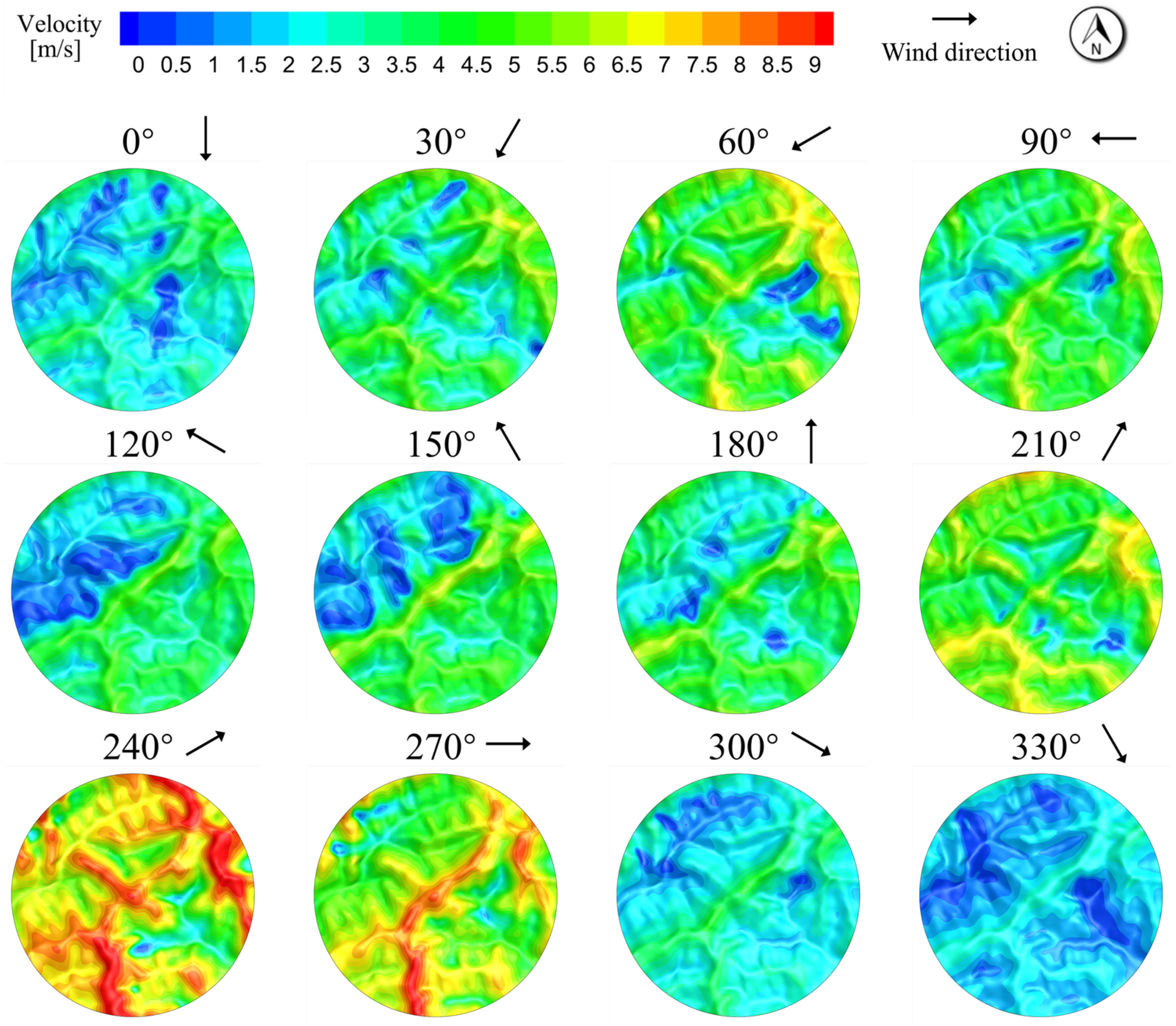
4.1.1. Mean Wind Speed

All visualizations in this study were generated using Tecplot 360 EX 2020 R1software. The velocity cloud map at 70 m above the ground surface under the 120° wind direction is shown in Figure 10. The wind speed variations in the complex terrain are quite significant, exhibiting strong spatiotemporal correlations. It can be observed that the overall wind speed in the flow field is mainly influenced by the inflow wind speed as a boundary condition. The wind speed is highest under the 240° wind direction, mostly ranging from 7 to 9 m/s, followed by the 270° wind direction. In contrast, the wind speed is lowest under the 330° wind direction, with values around of 1 m/s, with many areas showing ultra-low wind speeds. Due to the absence of obvious obstacles within the terrain, the maximum wind speed generally occurs along the ridge lines or on the hilltops. Regardless of the wind direction, the incoming wind is significantly obstructed by the mountainous terrain, forming low-speed wake zones on the leeward side. Particularly under the 120° and 150° wind directions, a distinct cut-off phenomenon occurs due to the influence of the ridge lines.

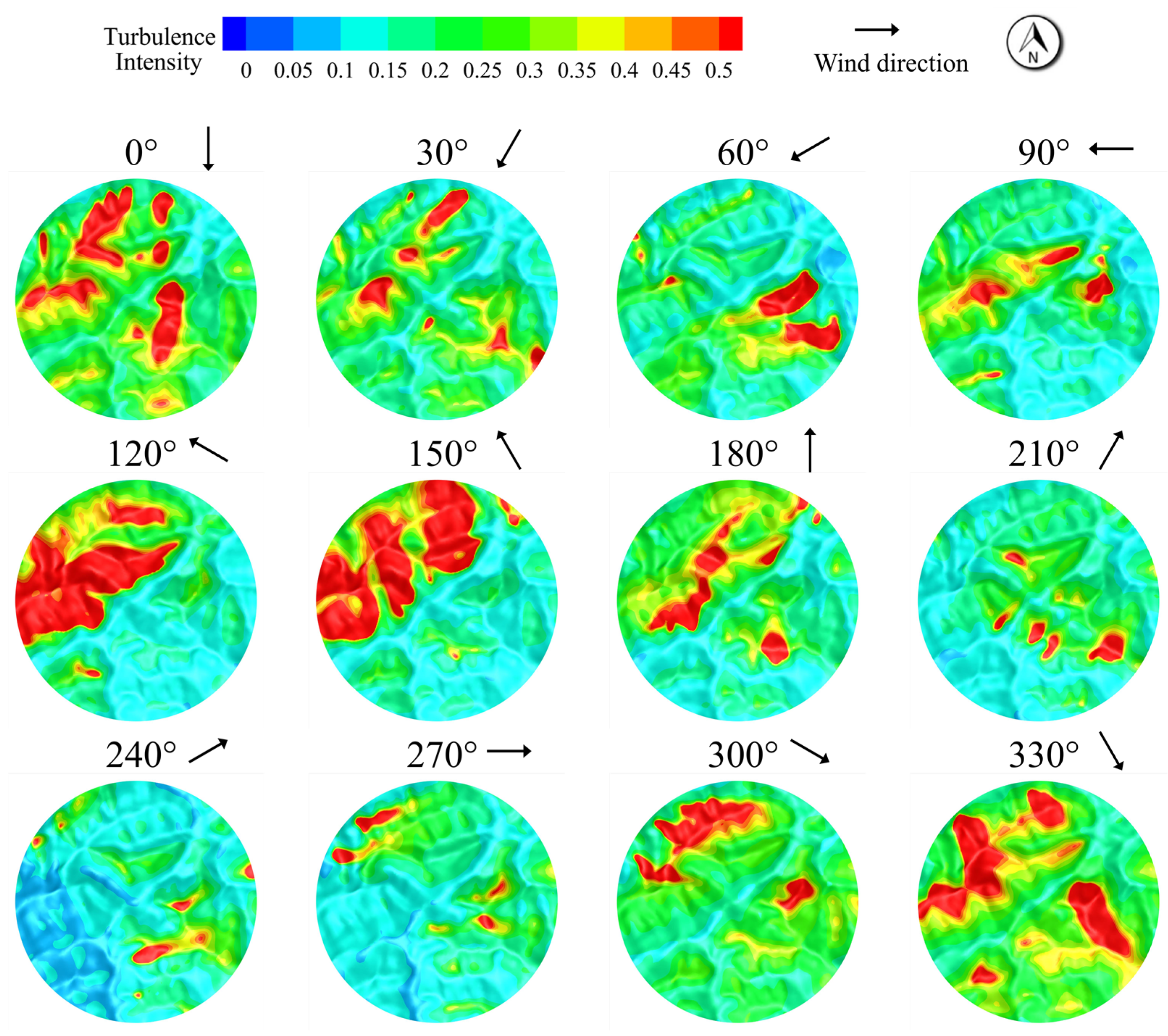
4.1.2. Turbulence Intensity

The numerical simulation of turbulence intensity at a height of 70 m above the surface for wind directions of 240° and 270° is shown in Figure 11. It can be observed that high turbulence areas correspond to low wind speed regions in Figure 10 (wind speed comprehensive map), indicating that lower wind speeds result in higher turbulence intensity. For wind directions of 240° and 270°, the wind speed values are relatively high, and the turbulence intensity values are relatively low. Additionally, turbulence intensity is significantly affected by terrain shielding effects, with values exceeding 0.5 behind ridgelines and mountain tops. High turbulence does not occur in relatively elevated positions where wind speeds are higher but is instead distributed at the mountain base and behind obstacles. In most cases, the turbulence intensity values are around 0.2.

4.2. Local Terrain Impact under the Same Wind Direction

4.2.1. Changes in Local Streamlines

To gain a more comprehensive understanding of the flow field characteristics in complex mountainous areas, it is essential to focus on how micro-topography influences local flow field changes. We selected a ridge perpendicular to the initial wind direction at 90° for this study. This ridge is near the terrain transition zone where the incoming wind has not been affected by other topographical features. The selected location is shown in Figure 12a. The streamline diagram is presented in Figure 12b. It can be observed that the wind speed gradually increases as it ascends the slope and reaches its maximum at the ridge top. After passing the ridge top, the incoming wind forms a local low-speed wake region behind the slope, where the wind speed decreases and the streamlines become more complex, indicating that the flow dynamics become more intricate (the front and back are determined by the direction of the incoming wind, with the area near the inlet being the front). In the same cross-section, the relative height of the rear ridge is lower than that of the front ridge, placing it within the low-speed wake region of the latter. Although the wind speed increases during the ascent of the rear slope, the speed at the ridge top is still lower than that of the front ridge top. This is partly due to the shielding effect of the front ridge’s terrain, which causes airflow separation, and partly because the ascent stage of the rear slope is shorter, preventing sufficient acceleration of the wind speed.

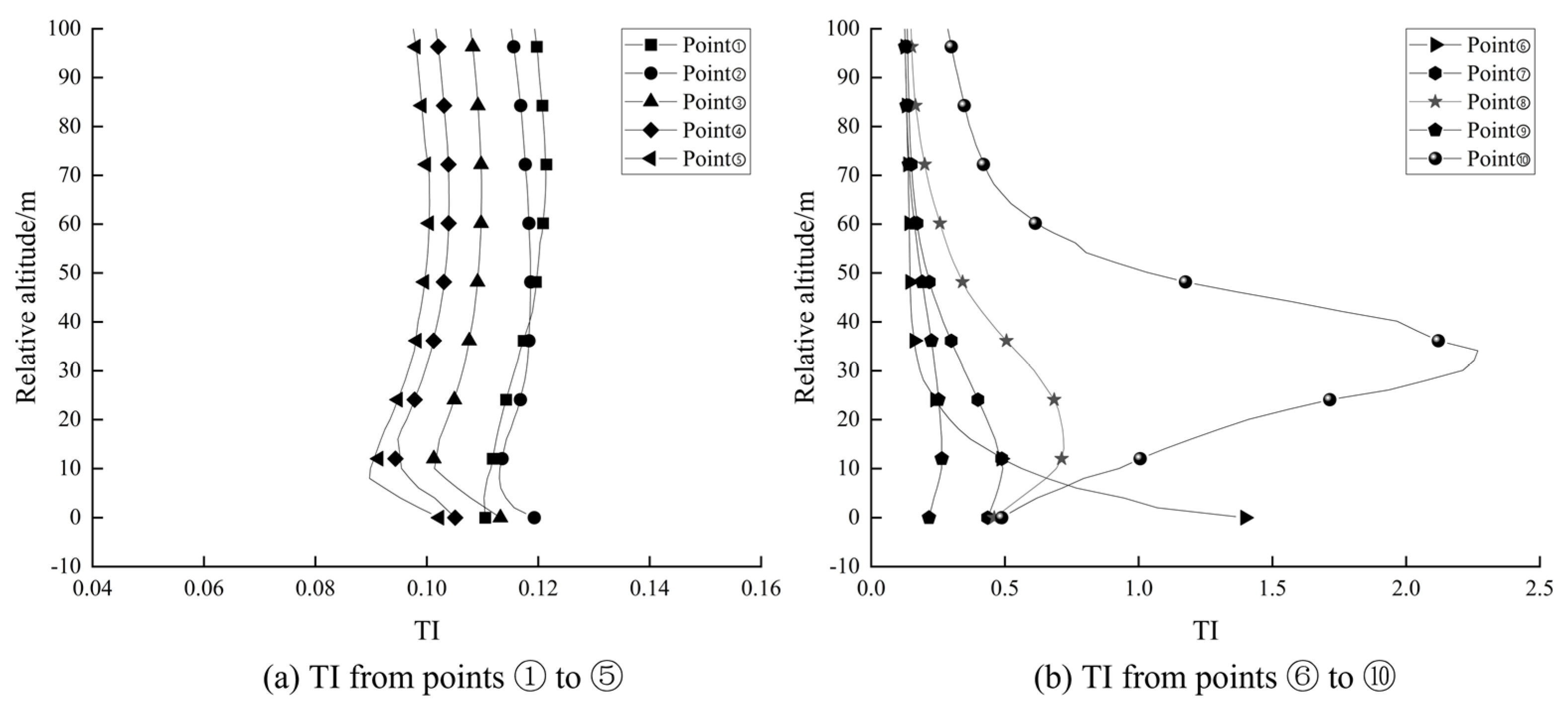
4.2.2. Local Turbulence Intensity

To monitor the variation of turbulence intensity influenced by terrain, ten measurement points were arranged on the same microtopography under a 90° wind direction, as shown in Figure 13. In terms of terrain distribution, measurement points ① to ⑤ and ⑦ to ⑨ are located on the windward slope, with point ⑤ being the highest point in the front mountain and point ⑨ being the highest in the rear mountain, while points ⑥ and ⑩ are on the leeward side. The vertical variation of turbulence intensity is shown in Figure 14, where the turbulence intensity decreases from low to high relative heights, due to the gradual reduction in the influence from the terrain and surface roughness. As seen in Figure 14a, during the ascent, the turbulence intensity decreases sequentially, reaching a minimum of about 0.98 at the hilltop, indicating an increase in wind speed and a decrease in turbulence intensity. In contrast, the turbulence intensities at the measurement points in Figure 14b are significantly higher than those shown in Figure 14a, because points ⑥ to ⑩ are all located in the low-speed wake region of the front mountain. The incoming wind separates on the leeward side, leading to increased turbulence intensity and greater flow field instability. Specifically, at point ⑩, which is affected by the two leeward slopes, the turbulence intensity reaches a maximum of 2.27. It is noteworthy that points ⑦ and ⑧ on the windward slope exhibit different turbulence intensity variations compared to points ① to ⑤. This discrepancy is due to the rear mountain being in the wake shadow of the front mountain, complicating the flow conditions. The flow field in complex terrains is easily influenced by the cumulative effect of continuous terrain changes, making it difficult to discern patterns. However, the turbulence intensity at point ⑨, also on a hilltop, is relatively low, which is consistent with the conclusion that higher wind speeds correspond to lower turbulence intensities.

5. Conclusions

This paper proposes a method to optimize the boundary conditions for numerical simulations in complex terrains, combining wind measurement data to better reflect real conditions. By applying this method to actual complex terrain wind farm modeling, performing CFD numerical simulations for accuracy verification, and exploring the characteristics of the flow field, the following conclusions are drawn:

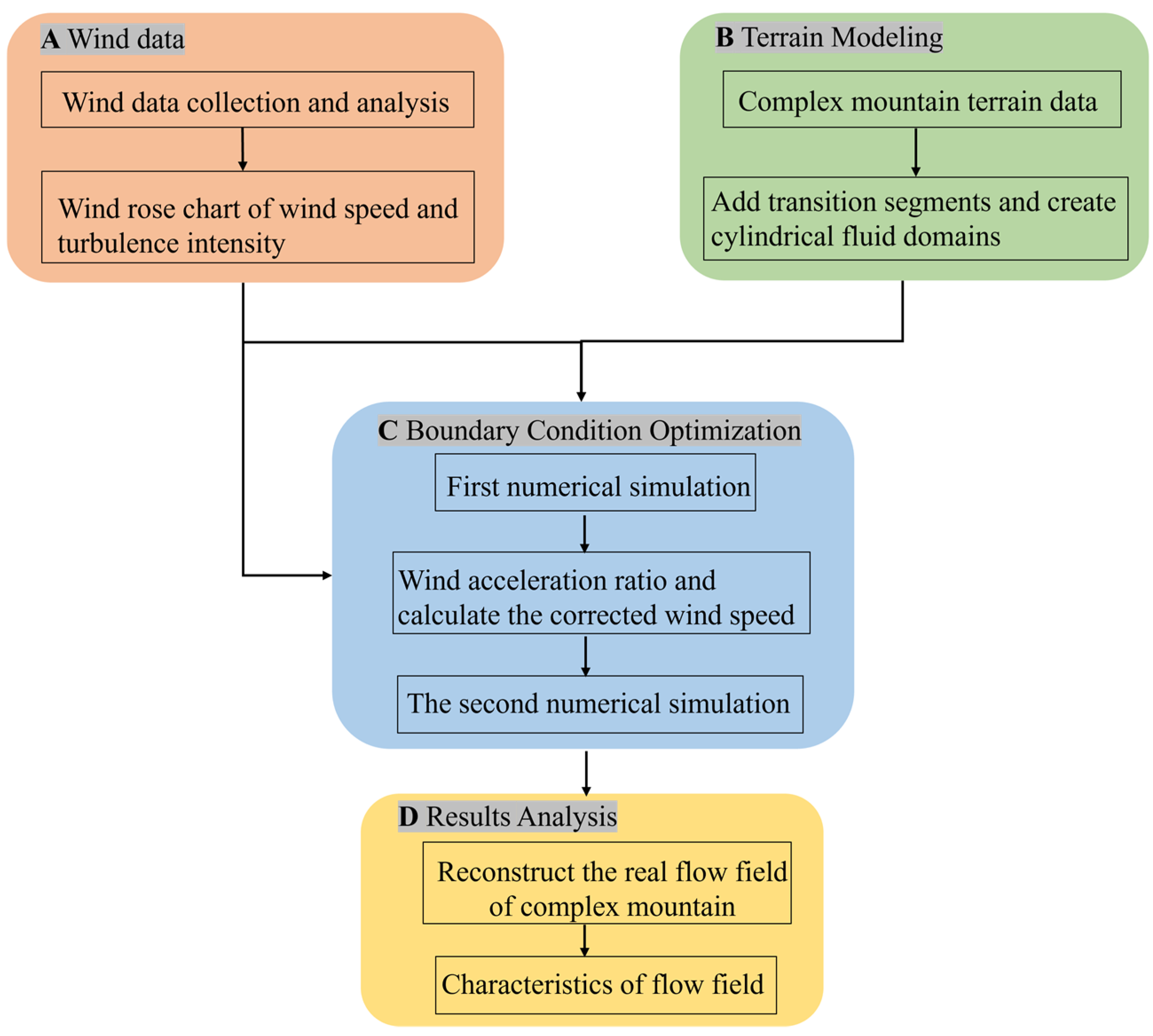
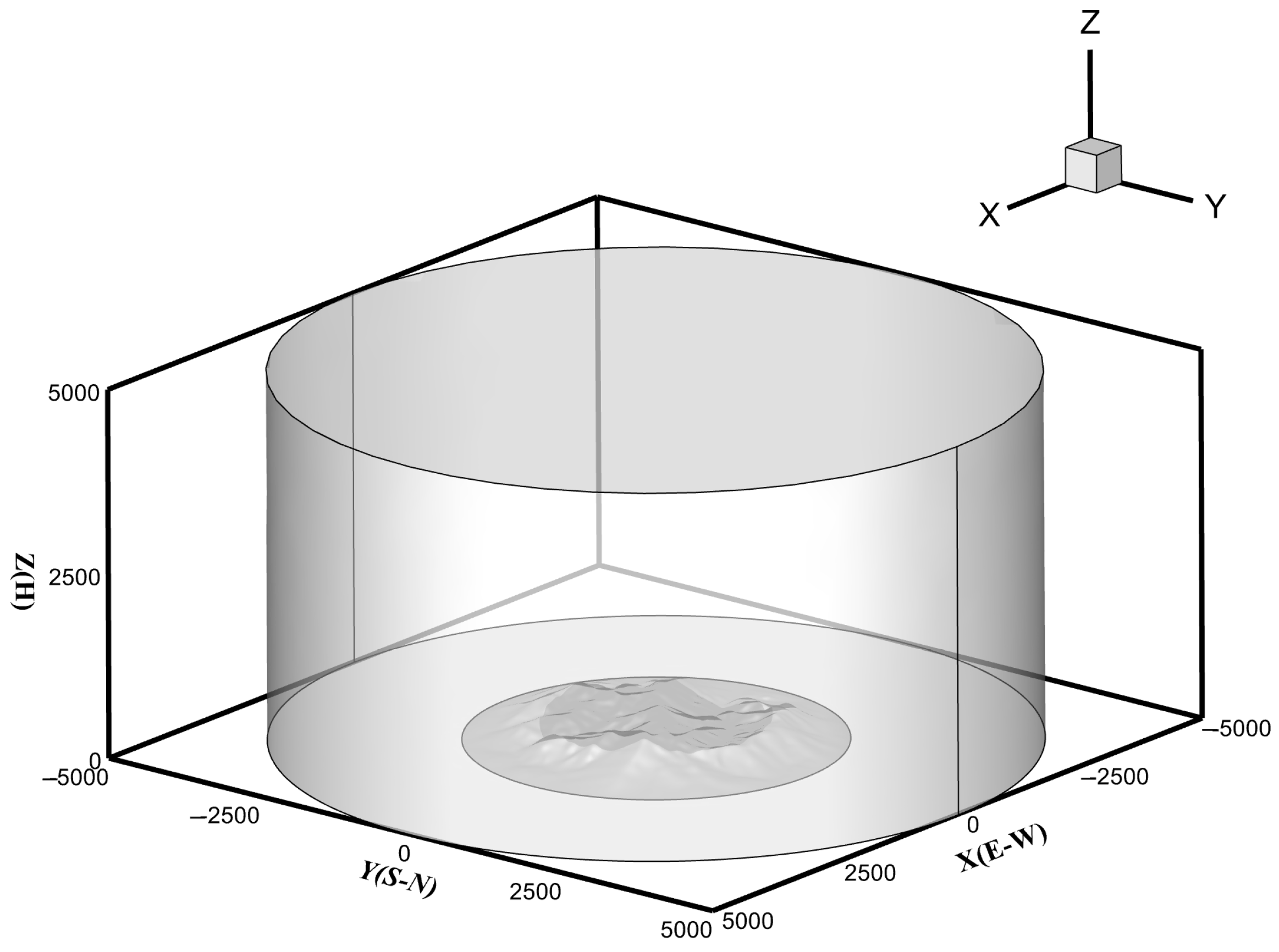
• Terrain Modeling: Considering the impact of “man-made cliffs”, a transitional curve that restores the original terrain variations within the transition section is used. To avoid grid errors, a cylindrical fluid domain is established, and the range of the inlet and outlet areas is flexibly selected to achieve wind direction conversion. In terms of boundary conditions, the inlet wind speed is corrected by the acceleration ratio to obtain a flow field distribution that is closer to reality.
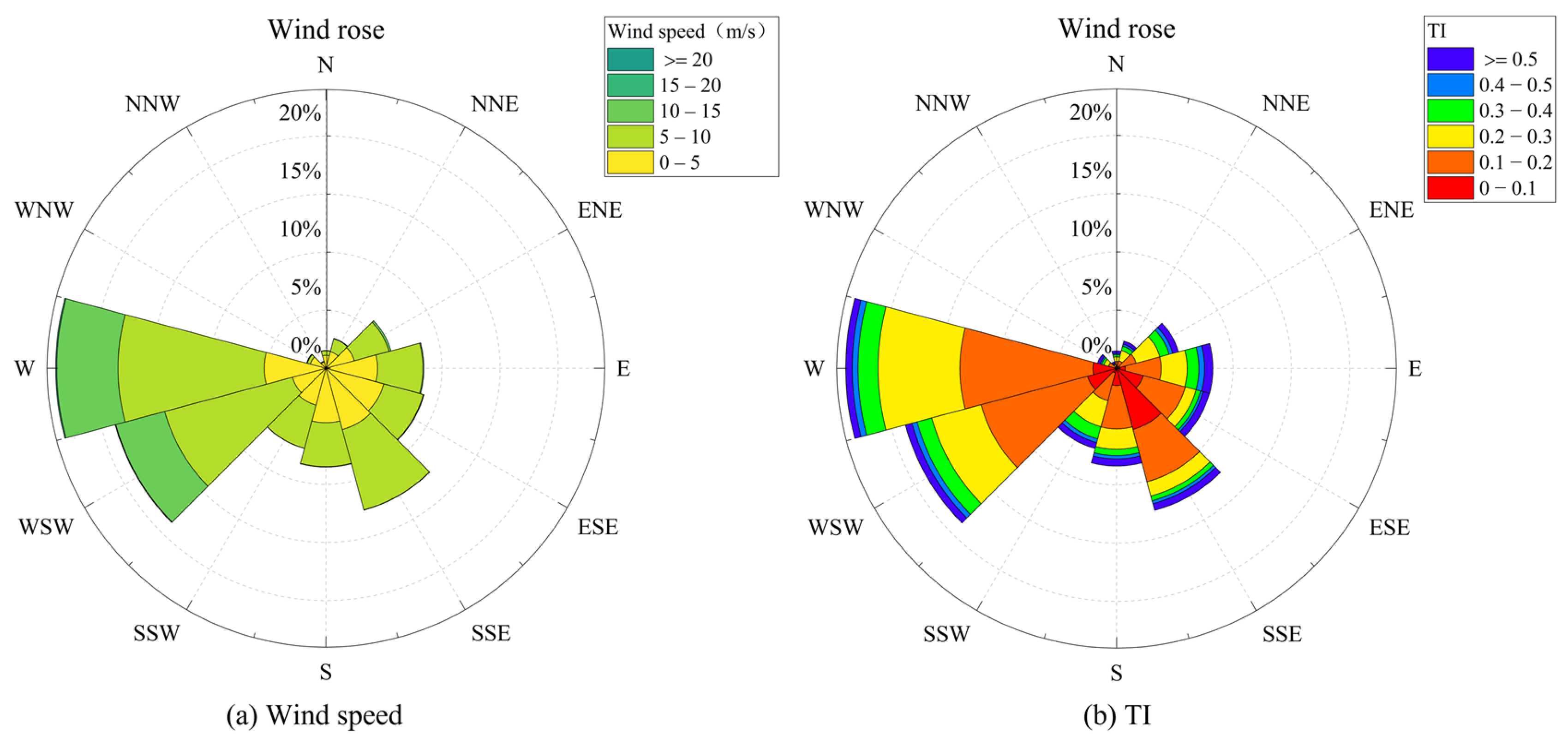
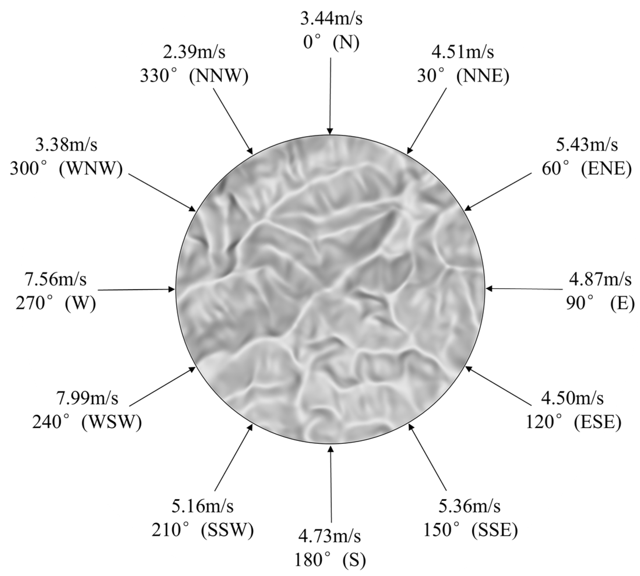
• Wind Measurement Data Analysis: The analysis of the wind measurement tower data shows a dominant wind direction concentrated in the W sector, accounting for 23.59% of occurrences, followed by the WSW and SSE sectors, with frequencies of 19.05% and 12.77%, respectively. Most wind speeds vary between 5 m/s and 10 m/s. Turbulence intensity mainly ranges from 0.1 to 0.3, generally indicating low to moderate turbulence intensity.
• Applicability of the New Method: The proposed method shows good applicability to complex terrain wind farms. Comparing numerical simulations with field-measured wind speed and direction, the wind speed error is within 6%, and the wind direction error is within 15°, indicating a certain degree of accuracy. Combining numerical simulations with measured data can recreate the actual flow field near the wind measurement tower, providing practical guidance for engineering.
• Flow Field Characteristics Comparison: Comparing the flow field characteristics under different wind directions reveals a significant terrain shielding effect on both wind speed distribution and turbulence intensity. The wind speed distribution and turbulence intensity are particularly evident under 120° and 150° wind directions, due to a ridge line in the terrain that is almost perpendicular to the incoming wind. When the incoming wind reaches the ridge or hilltop, it forms a low-speed wake region behind, where the wind speed decreases, the turbulence intensity increases, and the flow field becomes unstable.
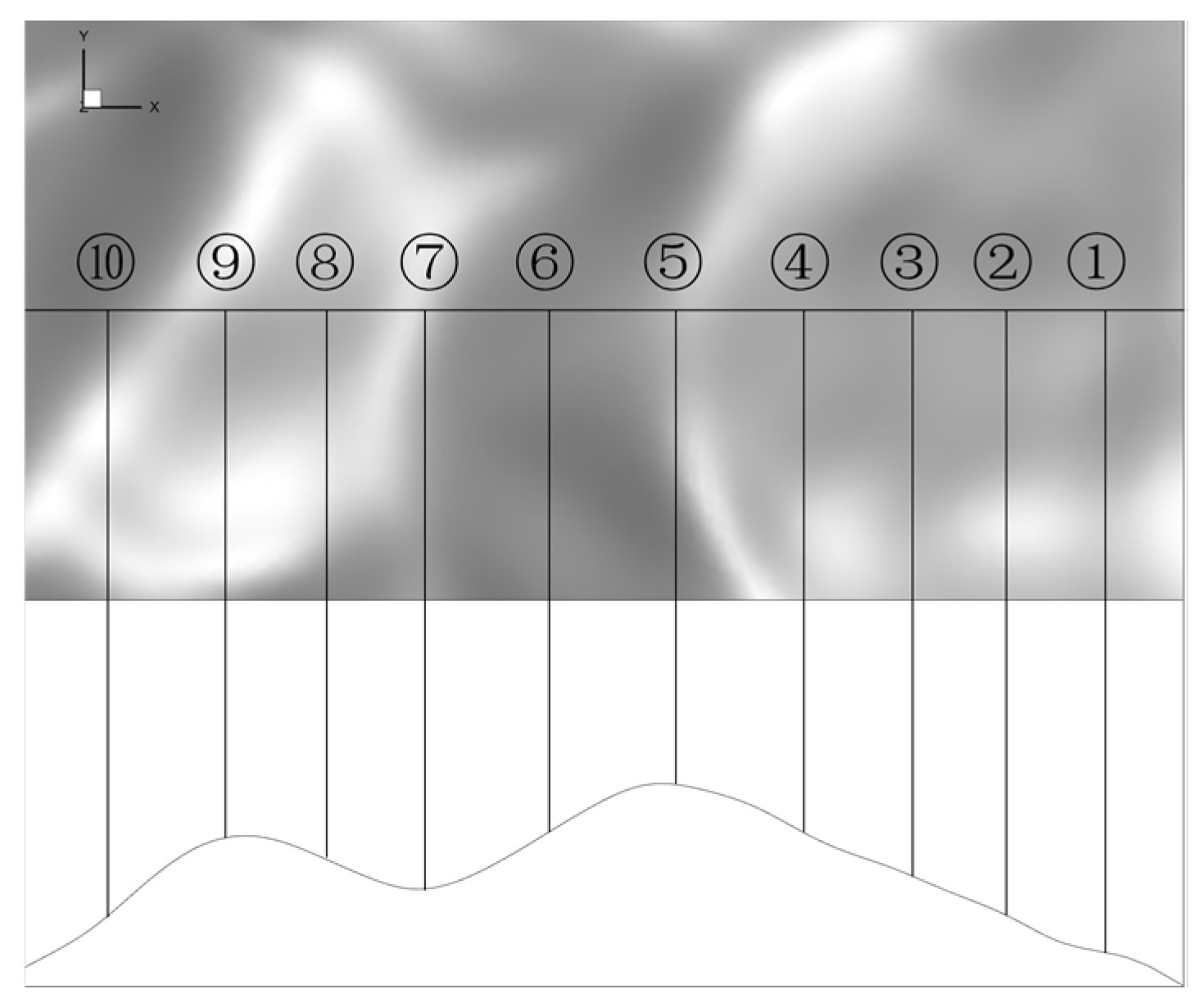
• Terrain Impact on Flow Field: To observe the terrain impact under the same wind direction, a ridge section almost perpendicular to the incoming wind and unaffected by other terrain features is selected. Changes in the lateral wind profile and turbulence intensity at the measurement points are observed. The results show that the flow field in complex terrains is significantly affected by terrain variations and the cumulative impact of continuous terrain changes, leading to inconsistent patterns. Overall, high-acceleration flow field regions are less affected by turbulence and eventually achieve higher wind speeds.

This method has been validated in a real wind farm case and can improve wind resource assessment and optimize fan placement, which can be used to improve efficiency. However, there is a limitation that the wind direction boundary conditions are not adjusted. Future work should consider the impact of different complex terrains on wind direction changes and conduct more related research.

References

1. Molla, S.; Farrok, O.; Alam, M.J. Electrical energy and the environment: Prospects and upcoming challenges of the World’s top leading countries. Renew. Sustain. Energy Rev. 2024, 191, 114177. [Google Scholar] [CrossRef]
2. Liu, J.; Song, D.; Li, Q.; Yang, J.; Hu, Y.; Fang, F.; Hoon Joo, Y. Life cycle cost modelling and economic analysis of wind power: A state of art review. Energy Convers. Manag. 2023, 277, 116628. [Google Scholar] [CrossRef]
3. Mark Hutchinson, Feng Zhao. GWEC|Global Wind Report 2023. Available online: https://gwec.net/globalwindreport2023/ (accessed on 24 June 2024).
4. Astolfi, D.; Castellani, F.; Terzi, L. A Study of Wind Turbine Wakes in Complex Terrain Through RANS Simulation and SCADA Data. J. Sol. Energy Eng. 2018, 140, 031001. [Google Scholar] [CrossRef]
5. Chen, F.; Wang, W.; Gu, Z.; Zhu, Y.; Li, Y.; Shu, Z. Investigation of hilly terrain wind characteristics considering the interference effect. J. Wind Eng. Ind. Aerodyn. 2023, 241, 105543. [Google Scholar] [CrossRef]
6. Berg, J.; Mann, J.; Bechmann, A.; Courtney, M.S.; Jorgensen, H.E. The Bolund Experiment, Part I: Flow Over a Steep, Three-Dimensional Hill. Bound.-Layer Meteorol. 2011, 141, 219–243. [Google Scholar] [CrossRef]
7. Kim, D.; Kim, T.; Oh, G.; Huh, J.; Ko, K. A comparison of ground-based LiDAR and met mast wind measurements for wind resource assessment over various terrain conditions. J. Wind Eng. Ind. Aerodyn. 2016, 158, 109–121. [Google Scholar] [CrossRef]
8. Assireu, A.T.; Pimenta, F.M.; de Freitas, R.M.; Saavedra, O.R.; Neto, F.L.; Júnior, A.R.T.; Oliveira, C.B.; Lopes, D.C.; de Lima, S.L.; Veras, R.B.J.E. EOSOLAR Project: Assessment of wind resources of a coastal equatorial region of Brazil—Overview and preliminary results. Energies 2022, 15, 2319. [Google Scholar] [CrossRef]
9. Shen, G.H.; Yao, J.F.; Lou, W.J.; Chen, Y.; Guo, Y.; Xing, Y.L. An Experimental Investigation of Streamwise and Vertical Wind Fields on a Typical Three-Dimensional Hill. Appl. Sci. 2020, 10, 1463. [Google Scholar] [CrossRef]
10. Zheng, K.; Tian, W.; Qin, J.; Hu, H. An experimental study on the turbulent flow over two-dimensional plateaus. In Proceedings of the 2018 Wind Energy Symposium, Kissimmee, FL, USA, 8–12 January 2018. [Google Scholar]
11. Radünz, W.C.; Mattuella, J.M.L.; Petry, A.P. Wind resource mapping and energy estimation in complex terrain: A framework based on field observations and computational fluid dynamics. Renew. Energy 2020, 152, 494–515. [Google Scholar] [CrossRef]
12. Castro, F.A.; Palma, J.; Lopes, A.S. Simulation of the Askervein flow.: Part 1: Reynolds averaged Navier-Stokes equations (k-ε turbulence model). Bound.-Layer Meteorol. 2003, 107, 501–530. [Google Scholar] [CrossRef]
13. Paiva, L.M.S.; Bodstein, G.C.R.; Menezes, W.F. Numerical simulation of atmospheric boundary layer flow over isolated and vegetated hills using RAMS. J. Wind Eng. Ind. Aerodyn. 2009, 97, 439–454. [Google Scholar] [CrossRef]
14. Dhunny, A.Z.; Lollchund, M.R.; Rughooputh, S. Wind energy evaluation for a highly complex terrain using Computational Fluid Dynamics (CFD). Renew. Energy 2017, 101, 1–9. [Google Scholar] [CrossRef]
15. Han, Y.; Stoellinger, M.; Naughton, J. Large eddy simulation for atmospheric boundary layer flow over flat and complex terrains. In Proceedings of the Conference on Science of Making Torque from Wind (TORQUE), Munich, Germany, 7 October 2016. [Google Scholar]
16. Li, T.; Liu, Z.; Wang, H.; Bian, W.; Yang, Q. Large eddy simulation for the effects of ground roughness and atmospheric stratification on the wake characteristics of wind turbines mounted on complex terrains. Energy Convers. Manag. 2022, 268, 115977. [Google Scholar] [CrossRef]
17. Diebold, M.; Higgins, C.; Fang, J.N.; Bechmann, A.; Parlange, M.B. Flow over Hills: A Large-Eddy Simulation of the Bolund Case. Bound. Layer Meteorol. 2013, 148, 177–194. [Google Scholar] [CrossRef]
18. Cheng, X.; Yan, B.W.; Zhou, X.H.; Yang, Q.S.; Huang, G.Q.; Su, Y.W.; Yang, W.; Jiang, Y. Wind resource assessment at mountainous wind farm: Fusion of RANS and vertical multi-point on-site measured wind field data. Appl. Energy 2024, 363, 123116. [Google Scholar] [CrossRef]
19. Rodrigues, C.V.; Palma, J.; Rodrigues, A.H. Atmospheric Flow over a Mountainous Region by a One-Way Coupled Approach Based on Reynolds-Averaged Turbulence Modelling. Bound. Layer Meteorol. 2016, 159, 407–437. [Google Scholar] [CrossRef]
20. Durán, P.; Meissner, C.; Casso, P. A new meso-microscale coupled modelling framework for wind resource assessment: A validation study. Renew. Energy 2020, 160, 538–554. [Google Scholar] [CrossRef]
21. Song, M.X.; Chen, K.; He, Z.Y.; Zhang, X. Wind resource assessment on complex terrain based on observations of a single anemometer. J. Wind Eng. Ind. Aerodyn. 2014, 125, 22–29. [Google Scholar] [CrossRef]
22. Yan, B.W.; Li, Q.S. Coupled on-site measurement/CFD based approach for high-resolution wind resource assessment over complex terrains. Energy Convers. Manag. 2016, 117, 351–366. [Google Scholar] [CrossRef]
23. Tang, X.Y.; Zhao, S.M.A.; Fan, B.; Peinke, J.; Stoevesandt, B. Micro-scale wind resource assessment in complex terrain based on CFD coupled measurement from multiple masts. Appl. Energy 2019, 238, 806–815. [Google Scholar] [CrossRef]
24. Maurizi, A.; Palma, J.M.L.M.; Castro, F.A. Numerical simulation of the atmospheric flow in a mountainous region of the North of Portugal. J. Wind Eng. Ind. Aerodyn. 1998, 74, 219–228. [Google Scholar] [CrossRef]
25. Hu, P.; Li, Y.L.; Huang, G.Q.; Kang, R.; Liao, H.L. The appropriate shape of the boundary transition section for a mountain-gorge terrain model in a wind tunnel test. Wind Struct. 2015, 20, 15–36. [Google Scholar] [CrossRef]
26. Ren, H.H.; Laima, S.J.; Chen, W.L.; Zhamg, B.; Guo, A.X.; Li, H. Numerical simulation and prediction of spatial wind field under complex terrain. J. Wind Eng. Ind. Aerodyn. 2018, 180, 49–65. [Google Scholar] [CrossRef]
27. Huang, G.Q.; Cheng, X.; Peng, L.L.; Li, M.S. Aerodynamic shape of transition curve for truncated mountainous terrain model in wind field simulation. J. Wind Eng. Ind. Aerodyn. 2018, 178, 80–90. [Google Scholar] [CrossRef]
28. Liu, Z.Q.; Ishihara, T.; He, X.H.; Niu, H.W. LES study on the turbulent flow fields over complex terrain covered by vegetation canopy. J. Wind Eng. Ind. Aerodyn. 2016, 155, 60–73. [Google Scholar] [CrossRef]
29. Castellani, F.; Astolfi, D.; Burlando, M.; Terzi, L. Numerical modelling for wind farm operational assessment in complex terrain. J. Wind Eng. Ind. Aerodyn. 2015, 147, 320–329. [Google Scholar] [CrossRef]
30. GB50009; Load Code for the Design of Building Structures. Urban-Rural Construction of the People’s Republic of China: Beijing, China, 2012.
31. Hu, W.C.; Yang, Q.S.; Chen, H.P.; Yuan, Z.T.; Li, C.; Shao, S.; Zhang, J. Wind field characteristics over hilly and complex terrain in turbulent boundary layers. Energy 2021, 224, 120070. [Google Scholar] [CrossRef]
32. Yamaguchi, A.; Ishihara, T.; Fujino, Y. Numerical modeling of local wind focusing on computational domain setting and boundary treatments. In Proceedings of the Fourth International Symposium on Computational Wind Engineering, Yokohama, Japan, 16–19 July 2006. [Google Scholar]
33. Blocken, B.; Stathopoulos, T.; Carmeliet, J. CFD simulation of the atmospheric boundary layer: Wall function problems. Atmos. Environ. 2007, 41, 238–252. [Google Scholar] [CrossRef]
34. He, J.W.; Zhang, H.F.; Zhou, L. Numerical Simulation of Wind Characteristics in Complex Mountains with Focus on Terrain Boundary Transition Curve. Atmosphere 2023, 14, 230. [Google Scholar] [CrossRef]
35. AIJ. RLB Recommendations for Loads on Buildings; Architectural Institute of Japan: Tokyo, Japan, 2004; pp. 611–613. [Google Scholar]
36. Abdi, D.S.; Bitsuamlak, G.T. Wind flow simulations on idealized and real complex terrain using various turbulence models. Adv. Eng. Softw. 2014, 75, 30–41. [Google Scholar] [CrossRef]
37. Blazek, J. Computational Fluid Dynamics: Principles and Applications; Butterworth-Heinemann: Oxford, UK, 2015. [Google Scholar]
38. Blocken, B.; van der Hout, A.; Dekker, J.; Weiler, O. CFD simulation of wind flow over natural complex terrain: Case study with validation by field measurements for Ria de Ferrol, Galicia, Spain. J. Wind Eng. Ind. Aerodyn. 2015, 147, 43–57. [Google Scholar] [CrossRef]
Figure 1. The whole process of numerical simulation.
Processes 12 01885 g001
Figure 2. Variation of complex mountain wind profile.
Processes 12 01885 g002
Figure 3. Wind roses in 12 winds.
Processes 12 01885 g003
Figure 4. The topography of the study area.
Processes 12 01885 g004
Figure 5. Cylindrical computing domain.
Processes 12 01885 g005
Figure 6. Computing domain grid.
Processes 12 01885 g006
Figure 7. Grid independence verification.
Processes 12 01885 g007
Figure 8. Working condition setting.
Processes 12 01885 g008
Figure 9. Numerical simulation accuracy verification.
Processes 12 01885 g009
Figure 10. Numerical simulation of velocity cloud images at 70 m altitude above the surface under 12 wind directions.
Processes 12 01885 g010
Figure 11. Numerical simulation of high turbulence intensity clouds over 70 m above the surface under 12 wind directions.
Processes 12 01885 g011
Figure 12. Terrain selection and flow line under 90° wind direction.
Processes 12 01885 g012
Figure 13. Point distribution.
Processes 12 01885 g013
Figure 14. Vertical variation of turbulence intensity at measuring point.
Processes 12 01885 g014