Production Prediction and Influencing Factors Analysis of Horizontal Well Plunger Gas Lift Based on Interpretable Machine Learning

Abstract

With the development of unconventional natural gas resources, plunger gas lift technology has gained widespread application. Accurately predicting gas production from unconventional gas reservoirs is a crucial step in evaluating the effectiveness of plunger gas lift technology and optimizing its design. However, most existing prediction methods are mechanism-driven, incorporating numerous assumptions and simplifications that make it challenging to fully capture the complex physical processes involved in plunger gas lift technology, ultimately leading to significant errors in capacity prediction. Furthermore, engineering design factors and production system factors associated with plunger gas lift technology can contribute to substantial deviations in gas production forecasts. This study employs three powerful regression algorithms, XGBoost, Random Forest, and SVR, to predict gas production in plunger gas lift wells. This method comprehensively leverages various types of data, including collected engineering design, production system, and production data, directly extracting the underlying patterns within the data through machine learning algorithms to establish a prediction model for gas production in plunger gas lift wells. Among these, the XGBoost algorithm stands out due to its robustness and numerous advantages, such as high accuracy, ability to effectively handle outliers, and reduced risk of overfitting. The results indicate that the XGBoost algorithm exhibits impressive performance, achieving an R² (coefficient of determination) value of 0.87 for six-fold cross-validation and 0.85 for the test set. Furthermore, to address the “black box” problem (the inability to know the internal working structure and workings of the model and to directly understand the decision-making process), which is commonly associated with conventional machine learning models, the SHAP (Shapley additive explanations) method was utilized to globally and locally interpret the established machine learning model, analyze the main factors (such as starting time of wells, gas–liquid ratio, catcher well inclination angle, etc.) influencing gas production, and enhance the credibility and transparency of the model. Taking plunger gas lift wells in southwest China as an example, the effectiveness and practicality of this method are demonstrated, providing reliable data support for shale gas production prediction, and offering valuable guidance for actual on-site production.

1. Introduction

In recent decades, unconventional natural gas resources have gradually emerged as a significant source of global energy supply. Both China and North America are witnessing highly active commercial exploitation of unconventional natural gas resources. Among these, shale gas and tight gas resources, which are primary components of unconventional resources, have become pivotal areas for natural gas production [1,2,3]. Shale gas reservoirs (carbonate reservoirs) typically employ the “horizontal well and volume fracturing” extraction technology. This technology is characterized by a rapid decline in early production, a prolonged period of low production, and the continuous return of fracturing fluid throughout the entire production cycle. Consequently, the implementation of water drainage and gas production technology needs to be initiated early and sustained throughout the entire gas reservoir development cycle. This makes the large-scale application of water drainage and gas production technology an indispensable phase in the middle and late stages of shale gas development [4]. The gas lift drainage gas production technology plays a crucial role in delaying gas well flooding, enhancing gas reservoir production conditions, and augmenting gas reservoir development benefits and recovery rates. Plunger gas lift technology has gained widespread use as an efficient method for natural gas extraction. However, due to the intricate geological characteristics and production dynamics of unconventional gas reservoirs, accurately predicting production capacity has become an urgent challenge that necessitates a prompt solution.

Accurately predicting the production capacity of plunger gas lift technology is crucial for optimizing the design and operation process, enhancing economic benefits, deepening our understanding of unconventional natural gas resource development, and promoting their efficient utilization. As the scale of unconventional resource development expands, accurate production capacity forecasting becomes even more significant in ensuring rational resource development and management. By identifying the key factors influencing production capacity, engineers can refine technical solutions, reduce production costs, and enhance overall operational efficiency. Currently, most capacity-prediction methods rely on mechanism-driven models, such as simulation techniques based on physical principles. However, these models often necessitate numerous assumptions and simplifications [5,6,7,8], making it challenging to fully capture the intricate physical processes involved in plunger gas lift technology, which can lead to substantial prediction errors. In recent years, the application of machine learning technology in natural gas extraction has gradually increased. Yet most studies have concentrated on black box models that offer limited direct guidance for specific operations and designs. For instance, while methods based on neural networks or deep learning may achieve higher prediction accuracy, their lack of transparency regarding the internal working mechanism of the model restricts their practical engineering applications.

The current research mainly faces the following problems:

• Mechanism-driven models have limitations. As the theoretical and practical understanding of plunger gas lift performance parameters has grown, significant improvements have been made in plunger gas lift technology. Approximate dynamic models have been developed to facilitate our understanding of plunger lift performance [6,7,8]. These studies offer a comprehensive analysis of various factors influencing plunger gas lift performance and provide essential guidelines for actual production, enabling quick and effective diagnosis to ensure optimal lift performance. However, owing to our insufficient understanding of the underlying mechanism, these models rely on numerous assumptions and simplifications, making it challenging for them to accurately predict production capacity. Furthermore, mechanism-driven models are complex and diverse, and verifying their accuracy and reliability is also quite difficult. Additionally, the data generated by these models may be artificially adjusted without an actual on-site basis, introducing a degree of subjectivity and potentially lacking universal applicability;
• The nature of machine learning models is often seen as a black box. Ajay Singh [9] utilized classification and regression tree (CART) technology to analyze actual field data from natural gas wells, proposing a method for root cause identification and production diagnosis based on operational data. The regression tree model swiftly identified well groups with either good or poor performance and offered improvement suggestions based on statistical analysis. It emphasized the importance of adding additional operating variables to enhance diagnostic effectiveness and suggested future work to improve the predictive ability of regression tree analysis. A. Ranjan et al. [10] optimized the gas lift rate to maximize daily hydrocarbon production by using an artificial neural network model, which exhibited better accuracy and performance than previous models. Naresh N. Nandola et al. [11] proposed an efficient optimization method for the plunger lift process in shale gas wells. By transforming time series data and manipulating variables, a reduced-order cyclic model was established to maximize daily production while meeting operational constraints. This was achieved by Junfeng Shi et al. [12] employing big data analysis and deep recurrent neural networks to study and select 11 parameters from more than 40,000 artificial lift wells of PetroChina. An effect evaluation function was established, the best artificial lift method was successfully selected, and a calculation result compliance rate of 90.56% was achieved in over 5000 gas wells. This provided a reliable, practical, and intelligent method for optimizing and selecting artificial lift. Thanawit Ounsakul et al. [13] utilized supervised machine learning methods to enhance the artificial lift well selection process, with the aim of minimizing life cycle costs and increasing production. The machine learning model can detect differences and continuously learn under dynamic conditions, offering a breakthrough artificial intelligence solution for the oil and gas industry. Tan Chaodong et al. [14] established a data-based optimal decision model by analyzing the production characteristics of plunger gas lift. The similarity weight was calculated through the K nearest neighbor algorithm, the production system was optimized, and drainage efficiency and production were significantly improved. Anvar Akhiiatdinov et al. [15] used machine learning methods to simulate gas production in plunger lift wells and proposed a neural network model with acceptable accuracy. The model can run quickly, monitor the gas flow rate of individual wells, and optimize the plunger lift cycle based on cumulative gas production. Nagham Amer Sami [16] successfully developed a model using machine learning algorithms such as decision tree regression, random forest regression, and K nearest neighbor regression. This model can predict the pipe pressure of artificial intermittent gas lift wells with an accuracy of over 99.9%. Although these machine learning models have enriched the prediction methods of gas lift technology and improved prediction accuracy, they lack interpretability and cannot easily provide practical guidance for engineering design.
• The lack of comprehensive methods is evident. Yukun Xie et al. [17] introduced an unsupervised clustering method based on the Transformer encoder to identify periodic points in plunger lift data. This approach achieves high-quality clustering through the autoencoder of a deep neural network and optimizes plunger lift parameters. Currently, few methods combine the advantages of mechanism-driven and data-driven approaches due to their fundamental differences. Mechanism-driven models emphasize theoretical foundations and physical explanations, while data-driven models focus on automatically extracting patterns and relationships from data. Effectively combining these two to leverage the physical interpretation ability of mechanism models and the prediction accuracy of data-driven models poses a complex challenge.

The current gap in plunger gas lift technology is the absence of a production capacity prediction model that offers both high prediction accuracy and interpretability. Thus, the research objective is to develop a model that comprehensively utilizes the strengths of mechanism-driven and data-driven methods, deeply analyzes key influencing factors [18,19], and achieves high accuracy and practicality.

To address these issues, this study collected production data from 33 plunger gas lift wells in a gas field (average wellbore flow pressure of 9.2 MPa and average temperature of 84.55 °C) in southwest China. The dataset included a variety of engineering and production features, totaling about 1800 groups. Features were selected using the Pearson coefficient and household information method, and the dataset was validated and analyzed using a six-fold cross-validation method. Upon thorough comparison and analysis of models like XGBoost, random forest, and support vector machine (SVR), the performance of each was evaluated in depth. Notably, both XGBoost and RF, being tree-based models, exhibit strong interpretability and possess the capability to directly establish a mapping relationship between data features and prediction outcomes. These models are ensemble models composed of multiple decision trees, utilizing a voting mechanism to improve prediction accuracy while retaining a certain degree of interpretability. However, given that tree models are still regarded as black box models, this study introduces the SHAP (Shapley additive explanation) value method. This machine learning explanation tool is used to measure the importance of global features [20]. The SHAP method, as a machine learning explanation technique, has also been widely used in oil and gas research [21,22,23,24]. This method enhances the interpretability of machine learning models, making such models easier to understand and accept, and improving their credibility and practicality. Through these methods, a comprehensive capacity forecasting model is constructed that not only provides high-precision forecasts, but also explains the mechanism of action of various influencing factors, offering theoretical guidance for actual on-site engineering design and operation. Through the aforementioned methods, a comprehensive plunger gas lift well production capacity-prediction model was constructed. The results of the study indicated that the XGBoost algorithm exhibited impressive performance, achieving an R² value of 0.87 for the six-fold cross-validation and 0.85 for the test set. Furthermore, the SHAP (Shapley additive explanation) method was employed for both global and local interpretations of the established machine learning model. The main factors influencing gas production were analyzed, which enhanced the credibility and transparency of the model. The development of this method not only enabled accurate prediction of natural gas production from plunger gas-lifted wells under various operating conditions, but also facilitated the analysis and explanation of the primary engineering or production factors affecting the production of such wells. It aids in addressing the timeliness, blindness, and randomness of production measure adjustments in actual field operations. Ultimately, it provides theoretical guidance for engineering design and optimization in practical field applications.

2. Methodology

Figure 1 is the workflow diagram of this article. It mainly includes 6 working steps:

(1)

Original data collection: The dataset comprises the primary engineering parameters that influence shale gas wells, along with indicators for evaluating their productivity. These engineering parameters primarily encompass dynamic factors, resistance factors, and volume factors [25]. Productivity refers to the gas production of shale gas wells;

(2)

Data preprocessing involves several steps. First, perform data cleaning, interpolate missing data, reduce data dimensions, and convert the data [26]. Subsequently, divide the preprocessed dataset into a training set and a test set. The division ratio typically ranges from 70% to 30% or 80% to 20%. In this paper, the data division ratio is 80% to 20%;

(3)

Feature selection aims to identify the optimal subset of features, eliminating those that are irrelevant or redundant. This process not only diminishes the feature count, but also enhances model accuracy and expedites running time. Furthermore, selecting genuinely pertinent features streamlines the model, facilitating our comprehension of the underlying data generation process. Given that machine learning frequently confronts the challenge of overfitting, where model parameters become overly reliant on training data, performing feature selection on the data is imperative to mitigate this issue;

(4)

Machine learning model. Use the divided training set data to establish the corresponding capacity model, mainly to find the optimal parameter values in the machine learning model. Commonly used methods include grid search, multi-fold cross-validation, and autonomous learning;

(5)

The evaluation of the capacity forecasting model involves assessing its accuracy using the test set data. Commonly employed accuracy metrics encompass the coefficient of determination (R²), mean absolute error (MAE), and mean square error (MSE). Based on these evaluation indicators, the machine learning algorithm demonstrating the highest predictive performance on the test set is chosen to establish the definitive capacity forecasting model;

(6)

Model interpretation: Based on the established optimal capacity forecasting model, the SHAP value method is used to provide global and local interpretations of the capacity forecast.

The above description encapsulates the primary workflow of this paper, with the black solid-lined box diagram highlighting the pivotal step. The dashed-lined box positioned on the right illustrates the process of feature selection, inclusive of both scenarios with and without mutual information. Three distinct models are subsequently trained utilizing feature data. Notably, the colored dashed lines signify feature selection sans mutual information, whereas the colored implementation denotes the inclusion of mutual information in the selection process. Following this, the prediction outcomes of these varying models are meticulously compared under identical feature selection conditions. Ultimately, the SHAP value method is leveraged to provide insightful interpretations of the model’s performance.

2.1. Mutual Information Method

Information volume is a measure of the probability of an event or variable occurring. Generally, the lower the probability of an event occurring, the greater the amount of information contained in the event. This is consistent with intuitive understanding. The rarity of an event corresponds to a greater amount of information contained due to the low probability of such an event occurring.

Entropy [27] is a measure of the stability of a system. It is actually the expectation or mean of the information content of all variables in a system.

For discrete variables, the corresponding formula is (Equation (1)):

$$H(X)={\displaystyle {\sum }_{x\in X}P(x)\log \frac{1}{P(x)}=-}{\displaystyle {\sum }_{x\in X}P(x)\log P(x)=-E\log P(x)}$$

(1)

The more unstable a system is, or the higher the uncertainty of events occurring, the higher its entropy.

For continuous variables, it can be understood as its probability density function, and the corresponding formula is (Equation (2)):

$$H(X)={\displaystyle \int P(x)\log \frac{1}{P(x)}dx}$$

(2)

where $H(X)$ corresponds to the information entropy of feature X and $P(x)$ corresponds to the probability density function of feature X.

Before obtaining mutual information, conditional entropy is introduced. When a random variable is given, the entropy of the system can be expressed using Equation (3).

$$H(Y|X)={\displaystyle \sum _{x\in X}P(x)H(Y|X=x)}={\displaystyle \sum _{x\in X}{\displaystyle \sum _{y\in Y}P(x,y)\log \frac{1}{P(y|x)}}}=-E\log P(Y|X)$$

(3)

where $P(x,y)$ is the joint probability density function of feature X and outcome Y, and $P(y|x)$ is the conditional probability density function of X for a given outcome Y. If outcome Y is known, then $H(Y|X)$ is the uncertainty in measuring feature X. The entropy relationship diagram is shown in Figure 2.

Mutual information is the degree to which the information of feature X reduces the uncertainty of information in result Y. As shown in Figure 3, it is the intersection of X and Y. The expression is as shown in Equation (4).

$$I(X;Y)=H(X)-H(X|Y)=H(X)+H(Y)-H(X,Y)$$

(4)

2.2. XGBoost Model

Chen Tianqi [28] formally introduced XGBoost (extreme gradient boosting) in 2016. This innovative algorithm is rooted in GBDT (gradient boosting decision tree) methodology. XGBoost functions as a powerful boosted tree model, seamlessly integrating numerous tree models to create a robust classifier. At its core, it employs the CART (classification and regression tree) model, enhancing its predictive capabilities.

2.2.1. CART Regression Tree

The CART regression tree assumes the structure of a binary tree and proceeds by continuously splitting the features. As an illustration, the current tree node undergoes a split based on the j-th eigenvalue. Specifically, samples with eigenvalues less than s are allocated to the left subtree, while samples with eigenvalues greater than s are assigned to the right subtree. This process is described by the corresponding Equation (5).

$$\{\begin{array}{l}{R}_1(j,s)=\left\{x|x(j)\le s\right\}\\ R_2(j,s)=\left\{x|x(j)>s\right\}\end{array}$$

(5)

The CART regression tree meticulously partitions the sample space along the feature dimension, where optimizing such a division poses an NP-hard problem. Consequently, the decision tree model adopts a heuristic approach to tackle this complexity. The objective function generated by a typical CART regression tree is as shown in Equation (6).

$${\displaystyle \sum _{x_i\in R_m}{(y_i-f(x_i))}^2}$$

(6)

Therefore, when solving for the optimal tangent feature j and the optimal tangent point s, it translates into solving the objective function presented in Equation (7).

$$\underset{j,s}{\min }\left[\underset{c_1}{\min }{\displaystyle \sum _{x_i\in R_1(j,s)}{(y_i-c_1)}^2+\underset{c_2}{\min }}{\displaystyle \sum _{x_i\in R_2(j,s)}{(y_i-c_2)}^2}\right]$$

(7)

By traversing all the splitting points across all features, the optimal splitting features and points can be identified, ultimately yielding a regression tree.

2.2.2. XGBoost Algorithm

The fundamental concept of this algorithm revolves around continually augmenting trees and executing feature splitting to foster growth. With each additional tree, a novel function is acquired, tailored to accommodate the residual from the preceding prediction. Upon completing the training phase and acquiring K trees, the process of predicting a sample score begins. Essentially, based on the sample’s unique attributes, it is assigned to a corresponding leaf node within each tree. Each of these leaf nodes is associated with a specific score. Ultimately, the scores attributed to each tree are simply aggregated to derive the predicted value for the sample. The mathematical representation of this model is illustrated in Equation (8).

$${\stackrel{\wedge }{y}}_i=\varphi (x_i)={\displaystyle \sum _{k=1}^K{f}_k(x_i)}$$

(8)

Here, $F=\left\{f(x)=w_{q(x)}\right\}(q:R^m\to T,w\in R^T)$, where $w_{q(x)}$ is the score of the leaf node q, $f(x)$ is one of the regression trees; i is the i-th sample, k is the k-th tree, and ${\stackrel{\wedge }{y}}_i$ is the predicted value of the i-th sample.

2.2.3. XGBoost Principle

The objective function of XGBoost is defined as Equation (9):

$$obj={\displaystyle {\sum }_{i=1}^{n}l(y_i,{\stackrel{\wedge }{y}}_i)}+{\displaystyle {\sum }_{k=1}^K\Omega (f_k)}$$

(9)

where ${\displaystyle {\sum }_{i=1}^{n}l(y_i,{\stackrel{\wedge }{y}}_i)}$ is the training loss and ${\displaystyle {\sum }_{k=1}^K\Omega (f_k)}$ is the complexity of the tree; $\Omega (f_k)=\gamma T+{\displaystyle \frac{1}{2}}\lambda {\left|\left|w\right|\right|}^2$.

The objective function encompasses two distinct components. The first component assesses the discrepancy between the predicted score and the actual score, while the second serves as the regularization term. This regularization term itself comprises two elements: T, which signifies the count of leaf nodes, and w, which represents the score assigned to each leaf node. The number of leaf nodes can be regulated, allowing for control over the magnitude of the leaf node scores, thereby preventing overfitting by ensuring that these scores do not become excessively large.

In the context described, the newly constructed tree aims to align with the residual error from the preceding prediction. Specifically, upon generating t trees, the cumulative prediction score can be formulated as per Equation (10).

$${\stackrel{\wedge }{y}}_i^{(t)}={\stackrel{\wedge }{y}}_i^{(t-1)}+f_t(x_i)$$

(10)

where $g_i$ is the first-order derivative and $h_i$ is the second-order derivative.

Since the residual of the prediction scores of the first $t-1$ trees and y has no effect on the optimization of the objective function, it can be directly omitted. The simplified objective function is shown in Equation (11):

$$\tilde{\iota }(t)={\displaystyle \sum _{i=1}^n\left[g_i{f}_t(x_i)+\frac{1}{2}{h}_i{f_t}^2(x_i)\right]}+\Omega (f_t)$$

(11)

The aforementioned equation encapsulates the cumulative loss function value across each sample. By reformulating this equation, the objective function can be transformed into a quadratic equation centered on the leaf node score, denoted as w. Upon determining the optimal value of w and its corresponding objective function value, it becomes feasible to directly derive both the optimal w and the objective function formula by employing the vertex formula (Equation (12)).

$$\{\begin{array}{l}{w}_j^{\ast }=-{\displaystyle \frac{G_j}{H_j+\lambda }}\\ Obj=-{\displaystyle \frac{1}{2}}{\displaystyle {\sum }_{j=1}^T\frac{{G_j}^2}{H_j+\lambda }+\gamma T}\end{array}$$

(12)

2.3. Shapely Value Method

The swift progression of computer science has led to the proposition and implementation of numerous machine learning prediction models across diverse industries. However, a significant challenge lies in the inability to reasonably analyze and interpret the input features of these models, often termed as “black box models”. To address this issue, the SHAP value method [29] emerged within the realm of machine learning. This method, inspired by game theory, falls under the category of model post-explanation techniques. Its fundamental principle involves calculating the marginal contribution of features to the model’s output, subsequently providing explanations for the “black box model” at both global and local levels. The SHAP value method constructs an additive explanation model where all features are considered as “contributors”. Typically, the feature subset constituted by a specific feature represents the weighted average of its contribution, and the marginal contribution can be derived using Equation (13). From a game-theoretic perspective, the game in this context is the prediction of natural gas production based on the dataset.

$${\varphi }_j(f)={\displaystyle \frac{1}{\left|F\right|}}{{\displaystyle \sum _{S\subseteq F\backslash \{j\}}(\frac{\left|S\right|!(\left|F\right|-\left|S\right|-1)!}{\left|F\right|!})}}^{-1}(v(S\cup \{j\})-v(S))$$

(13)

where ${\varphi }_j(f)$ is the contribution of feature j, f is the model to be explained, $F\backslash \{j\}$ is the feature set without feature j, S is a subset of $F\backslash \{j\}$, $S\cup \{j\}$ is the subset S containing feature j, $\left|F\right|$ is the total number of features, and $\left|S\right|$ is the number of features in the subset.

2.4. Error Metric Method

To mitigate bias stemming from dataset partitioning and optimize its utilization, a six-fold cross-validation approach is adopted during model training and testing. This methodology partitions the training dataset into six subsets, with one subset serving as the test data in each cross-validation iteration, while the remaining five subsets are utilized for training. The cross-validation process iterates six times, and the model’s final performance is determined by averaging these scores (Figure 4).

Among them, 80% of the data is allocated for the cross-validation process, while the remaining 20% comprises the test set for the training samples. In simpler terms, the latter 20% of the data is excluded from any cross-validation step.

The output results undergo evaluation utilizing the mean-square error (MSE), root-mean*square error (RMSE), mean-absolute error (MAE), and coefficient of determination (R²). These assessment methods are mathematically represented as detailed in Equations (14)–(17).

$$MSE={\displaystyle \frac{1}{N_{test}}}{\displaystyle \sum _{i=1}^{N_{test}}{{\displaystyle (y_{pred}^i-y_{ture}^i)}}^2}$$

(14)

$$RMSE={\left({\displaystyle \frac{1}{N_{test}}}{\displaystyle \sum _{i=1}^{N_{test}}{{\displaystyle (y_{pred}^i-y_{ture}^i)}}^2}\right)}^{1/2}$$

(15)

$$MAE={\displaystyle \frac{1}{N_{test}}}{\displaystyle \sum _{i=1}^{N_{test}}\left|y_{pred}^i-y_{ture}^i\right|}$$

(16)

$$R^2=1-{\displaystyle \frac{{\displaystyle \sum _{i=1}^{N_{test}}{{\displaystyle (y_{pred}^i-y_{ture}^i)}}^2}}{{\displaystyle \sum _{i=1}^{N_{test}}{{\displaystyle (y_{true}^i-y_{average}^i)}}^2}}}$$

(17)

where $y_{ture}^i$ is the i-th true value, $y_{pred}^i$ is the i-th predicted value, $y_{average}^i$ is the mean of the true values, and $N_{test}$ is the total number of test data points.

3. Data Evaluation

China’s primary shale gas production regions are currently situated in the southwest. As of 2019, this region boasts confirmed shale gas reserves of 361.22 billion m³, with the gas-bearing area spanning 434.13 km². However, due to large-scale fracturing and shale gas production, the initial gas output is high but subsequently decreases, accompanied by a significant increase in liquid accumulation. In response to this challenge, plunger gas lift drainage gas production technology has demonstrated favorable results.

Given the complexity of wellbore structures and the variability of production dynamics, it is proposed to utilize machine learning methods to analyze historical dynamic data, such as casing pressure, in order to predict future gas production. This method will offer a valuable reference for adjusting the production system and aid in optimizing the production process. By learning from historical data, the model can forecast the trend of future gas production and provide timely, accurate information for production adjustments. This intelligent prediction system can enhance production efficiency while mitigating risks during the production process. Through real-time monitoring and data analysis, a better understanding of the well’s operating status can be gained, operations can be promptly adjusted, and the economic benefits of shale gas production can be maximized. Therefore, machine learning methods hold great potential for optimizing the shale gas production process.

3.1. Statistical Data Description

This dataset encompasses 11 features, including the shut-in casing pressure, shut-in tubing pressure, open-well casing pressure, and open-well tubing pressure. In instances of missing data (refer to Figure 5 for specifics), the absences were addressed, and ultimately, approximately 1800 features were retained for thorough analysis. Comprehensive details of the data features are available in

Table 1. Statistics of the dataset.

Name	Shut-in Casing Pressure (MPa)	Shut-in Tubing Pressure (MPa)	Open-Well Casing Pressure (MPa)	Open-Well Tubing Pressure (MPa)	Transfer Pressure (MPa)	Catcher Depth (m)
Mean	4.98	4.55	4.57	2.48	2.41	3.34
Std	1.11	1.00	1.07	0.80	0.70	0.17
Min	3.22	1.95	2.92	1.49	0.00	3.11
25%	4.25	3.89	3.86	2.02	2.01	3.20
50%	4.64	4.25	4.24	2.22	2.16	3.27
75%	5.76	5.07	5.25	2.64	2.54	3.50
Max	7.93	7.77	7.81	7.02	5.30	3.62

and

Table 2. Statistics of the dataset.

Name	Starting Time of Wells (h)	Time to Close the Wells (h)	Plunger Rising Time (h)	GLR (104 m3/m3)	Catcher Well Inclination Angle (°)	Gas Production (104 m3/d)
Mean	4.59	1.34	1.27	1.69	64.12	2.53
Std	6.31	0.46	0.54	0.69	3.03	1.12
Min	0.33	0.92	0.10	0.17	54.78	0.00
25%	1.00	1.00	1.00	1.19	63.38	1.77
50%	1.67	1.25	1.00	1.58	65.00	2.48
75%	4.50	1.50	1.50	2.04	66.18	3.21
Max	35.00	6.00	6.00	4.47	67.86	6.54

, while Figure 6 showcases the specific data pertaining to each feature. This dataset presents pivotal production parameters, including crucial aspects like the casing pressure and oil pressure at the wellhead. By meticulously examining these features, one can gain a deeper insight into the production dynamics of plunger gas lift technology in shale gas wells. This, in turn, enhances our overall comprehension of the production process and furnishes a more solid foundation for subsequent machine learning analyses.

Figure 5 illustrates the percentage of missing data. The GLR (gas–liquid ratio) exhibited more than 0.06% missing values, while the plunger rising time, gas production, open-well casing pressure, open-well tubing pressure, and transfer pressure all had no more than 0.01% missing data [30]. Given that the overall amount of missing data was minimal, it was decided to remove the missing data items from these data tables, leaving a total of 1800 data items.

3.2. Feature Selection

Figure 7 displays the Pearson correlation coefficients for all possible two-variable combinations, including gas production. According to the criteria established by Profillidis and Botzoris [31], a Pearson correlation coefficient greater than 0.85 signifies a high correlation between the two variables. A coefficient between 0.4 and 0.6 indicates a moderately strong correlation, while a coefficient less than 0.4 suggests a weak correlation [32,33]. When focusing on gas production (GP) as the primary analysis object, it was observed that gas production exhibited a moderately strong correlation with well opening time (0.65), shut-in tubing pressure (0.63), gas–liquid ratio (0.55), and shut-in casing pressure (0.47).

A strong linear relationship (0.77) existed between external delivery pressure and well opening tubing pressure, indicating that the external delivery pressure had a significant impact on wellhead tubing pressure. Notably, at the moment of well opening, external pressure can trigger a chain reaction within the plunger gas lift well system, further influencing the gas production performance. Additionally, there was a positive correlation between the shut-in time and locking device depth, suggesting that an increase in locking device depth may result in a prolongation of the well opening time. Similarly, a positive correlation exists between the plunger upward travel time and locking device depth, indicating that the plunger upward travel time may increase as the locking device depth increases. It is also noteworthy that there was a certain positive correlation between shut-in tubing pressure and shut-in casing pressure, as well as between the shut-in tubing pressure and opening casing pressure, further highlighting the mutual influence among these parameters in wellhead operations. Figure 8 elegantly illustrates the mutual information values of 11 pivotal features. These features, each making a substantial contribution to the prediction model, have been meticulously selected as the input indicators for the model. Given the profound interactions among these features, their incorporation enables a more comprehensive grasp of the system’s intricacies, thereby enhancing model performance and prediction accuracy.

4. Results and Discussion

4.1. Model Capacity Forecast

After feature selection, the input dataset comprised 11 distinct features. From the total 1800 production data points, 1440 (80%) were allocated for model training, while the remaining 360 data points (20%) were reserved as test data to assess the model’s performance.

Table 3. Comparison of models with mutually informative feature selection.

	With Mutual Information Feature Selection
	Cross-Validation Test Result			Test Set Result
	XGBoost	RF	SVR	XGBoost	RF	SVR
RMSE	0.38	0.35	0.44	0.37	0.41	0.51
MAE	0.21	0.23	0.27	0.17	0.19	0.29
R2	0.87	0.87	0.82	0.85	0.83	0.77
MSE	0.15	0.17	0.19	0.14	0.18	0.26

offers a comparative analysis of the performance of three models, utilizing mutual information for feature selection. By evaluating the performance of these models, one can discern which one excels on a specific dataset, ultimately facilitating more reliable guidance for production adjustments and strategic decisions.

After applying mutual information for feature selection, all models exhibited commendable performance. Specifically, in the XGBoost model, the determination coefficient (R²) for the six-fold cross-validation dataset was 0.87, and the determination coefficient (R²) for the test dataset was 0.85. While the support vector regression model (SVR) also demonstrated satisfactory performance, it exhibited certain limitations on the test dataset, achieving a determination coefficient (R²) of 0.77. Overall, the XGBoost model surpassed both the random forest model (RF) and the support vector regression model (SVR). These outcomes indicate that the XGBoost model can more precisely identify patterns and trends within production data, particularly when factoring in feature selection. The elevated determination coefficient value suggests that the model can adeptly explain variations in production data, thus offering reliable predictive capabilities. Furthermore, following the mutual information feature selection process.

After applying the mutual information method, Figure 9, Figure 10 and Figure 11 present the error statistics of the XGBoost, RF, and SVR models on the test set. The central panel depicts the residual, signifying the discrepancy between the predicted and actual values for each sample.

As evident in Figure 9b and Figure 10b, the errors of both the XGBoost and random forest (RF) models were generally evenly spread within the range of −0.5 to 0.5. Despite the XGBoost model’s robust generalization capabilities, which minimized the likelihood of significant errors in predicting unseen datasets, there was a notable outlier with an error exceeding −4. Specifically, for this outlier, the XGBoost model predicted 5.15 × 10⁴ m³/d, while the RF model predicted 6.23 × 10⁴ m³/d, against the actual value of 3.05 × 10⁴ m³/d, resulting in errors of 2.1 × 10⁴ m³/d and 3.18 × 10⁴ m³/d, respectively. Both models underestimated the actual plunger rise time, indicating a potential operational issue, such as plunger jamming, at this point, which led to inflated flow predictions.

In contrast, the support vector machine (SVR) model’s errors were more concentrated around ±1, as depicted in Figure 11b. However, the RF model struggled with accuracy in predicting certain samples, with five samples exhibiting errors exceeding 4. Despite achieving a parasitic R² value of 0.82 on cross-validation data, the RF model’s performance on the test dataset was suboptimal, attributed to its limited generalization ability. For the most significant error point, the predicted value was 2.5 × 10⁴ m³/d, whereas the actual value was 5.73 × 10⁴ m³/d, yielding an absolute error of 3.23 × 10⁴ m³/d. This discrepancy can be attributed to the unusually long well opening time of 23 h, significantly higher than the average of 4.59 h across all samples, which hindered the RF model’s ability to accurately capture the target characteristics.

4.2. SHAP Value Interpretation Model Based on Mutual Information

In this section, owing to the suboptimal performance of the SVR model, two tree-based models-namely the XGBoost model and the RF model-will be elucidated. Both of these methodologies employ the mutual information method for feature selection prior to training, and the SHAP value method is employed for comparative purposes.

4.2.1. XGBoost

Figure 12a illustrates the feature importance graph of the XGBoost model. Notably, the starting time of wells (STW) emerges as the primary determinant of gas production, followed by GLR. Specifically, the coefficient of GLR is 0.19. The top five influential factors include the starting time of wells, GLR, time to close the well, catcher well inclination angle, and shut-in tubing pressure.

Figure 12b presents a SHAP summary diagram of the XGBoost model, primarily comprising the test set data, organized by feature importance from top to bottom. This diagram offers a more intricate and informative view of SHAP values, revealing not only the relative importance of features, but also their actual relationship with the predicted outcomes. The color spectrum represents the variable value, with the transition from blue to red indicating an increase in the variable value. Positive (negative) SHAP values signify a positive (negative) correlation between the influencing parameter and gas production.

The first critical feature is the starting time of wells, exhibiting the widest distribution range along the horizontal axis and the highest feature importance. This parameter exerted the greatest influence on the model. Longer well opening times were associated with positive SHAP values (red data points extending to the right), implying a potential correlation with higher gas production. Conversely, shorter well opening times exhibited negative SHAP values (blue data points extending to the left), suggesting a possible association with lower gas production. Overall, the model interpreted the impact of well opening time on gas production as follows: longer durations may be linked to higher gas production, while shorter durations may be associated with lower gas production.

As the second most influential factor, changes in the GLR (gas-liquid ratio) have a substantial impact on the model. A larger GLR yields a positive SHAP value, indicating a positive impact on the model’s prediction results. The suggestion is that a higher gas-liquid ratio may be associated with increased gas production. Conversely, a smaller GLR yields a negative SHAP value, implying that a lower gas-liquid ratio may be correlated with decreased gas production.

The third most significant factor is the shut-in time. A shorter shut-in time exhibits a positive SHAP value, indicating a positive impact on the model’s prediction results. This suggests that a shorter shut-in time may be associated with higher gas production. Conversely, a longer shut-in time yields a negative SHAP value, indicating a negative impact on the model’s prediction results. This indicates that a short shut-in time may be linked to higher gas production, while a longer shut-in time may be associated with lower gas production.

The fourth crucial factor pertains to the catcher well inclination angle. The diagram illustrates that the SHAP values corresponding to this angle predominantly consisted of red data points, suggesting a potential correlation between a greater well inclination angle and enhanced gas production. This suggests that, in some cases, increasing the well inclination angle may positively impact gas production.

The fifth most important factor is shut-in tubing pressure, which behaves similarly to the GLR. A higher shut-in tubing pressure may be linked to a higher gas production rate, while a lower shut-in tubing pressure may be associated with a lower gas production rate. From the XGBoost perspective, the latter three factors are mostly concentrated around 0, indicating that these effects do not significantly impact the model’s output.

Figure 13 employs colors to depict the direction of each feature’s impact on the gas production forecast. Red arrows signify that the feature elevates the forecast, whereas blue arrows indicate that it diminishes the forecast. In this specific well, four features, including the gas–liquid ratio (GLR), increase the forecast, while several others, such as the time to close the well (TCW), decrease the forecast. Furthermore, the length of the arrow signifies the extent of the feature’s impact on the output; a longer arrow indicates a greater impact. The scale value on the X-axis allows for a quantitative assessment of the reduction or increase in impact. It is noteworthy that all features in this well exhibit a positive increase.

Ultimately, the predicted gas production of the well is 3.14 × 10⁴ m³/d, which closely aligns with the actual value of 2.85 × 10⁴ m³/d, yielding an absolute error of 9.23%. This demonstrates that the XGBoost model possesses a relatively high predictive accuracy for the well’s gas production. Locally interpreting Figure 13 yields a deeper understanding of how various features influence gas production during the actual production process.

4.2.2. Random Forest

Figure 14a illustrates the feature importance graph of the random forest model. The dominant factor influencing gas production is the starting time of wells (STW). Another significant factor is the open-well casing pressure, with a coefficient of 0.54. The top five influencing factors are the starting time of wells, open-well casing pressure, gas–liquid ratio (GLR), catcher well inclination angle, shut-in casing pressure, and shut-in tubing pressure.

The SHAP summary diagram of the random forest model (Figure 14b) reveals the impact of various factors on gas production. Factors such as the starting time of wells, open-well casing pressure, gas–liquid ratio (GLR), catcher well inclination angle, shut-in casing pressure, shut-in tubing pressure, and open-well tubing pressure exhibit positive correlation, indicating that changes in their numerical values may positively impact gas production. The remaining four factors show negative correlation, suggesting that an increase in these factors may lead to a decrease in gas production. This positive correlation phenomenon may indicate that the model has a weak generalization ability on new data, as it lacks a firm grasp of the influence relationship between different factors. Therefore, when using the random forest model to predict gas production, it is crucial to carefully consider the potential over- or under-prediction of the model.

The local interpretation of Figure 15 demonstrates the corresponding gas production prediction by the random forest model in practical application. The average gas production predicted by the random forest model is 2.634 × 10⁴ m³/d. In this specific well, seven features, including the gas–liquid ratio (GLR), contributed to increasing the prediction, while several other features decreased the prediction. Additionally, in this well, the length of the arrow indicates the magnitude of the feature’s impact on the output. The decrease or increase in impact can be observed through the scale value on the X-axis. Ultimately, the predicted gas production value of the well was 6.15 × 10⁴ m³/d, with a true value of 4.55 × 10⁴ m³/d, resulting in an absolute error of 26.02%. The significant error and poor prediction accuracy suggest a large deviation from the true value, which may be attributed to the model’s inaccurate understanding of certain factors or its relatively weak generalization ability to new data.

5. Conclusions

With the widespread application of machine learning in researching gas lift drainage gas production technology, this study aims to predict the gas production of plunger gas lift wells based on measured production data and engineering data. Addressing the challenges related to feature selection, data set size, and model interpretation, the mutual information method was employed for feature selection and three machine learning models (XGBoost, random forest, and SVR) were established for predicting production capacity. Ultimately, the two tree models (XGBoost and random forest) were thoroughly explained and compared using the SHAP value method. The following are the main conclusions of this paper:

(1)

This study is the first to attempt to combine the advantages of mechanism-driven and data-driven approaches in plunger lift technology. By integrating the XGBoost model with the SHAP value interpretation method, the accuracy and interpretability of plunger lift production predictions were improved. This method not only captures complex nonlinear relationships, but also provides a transparent physical explanation.

(2)

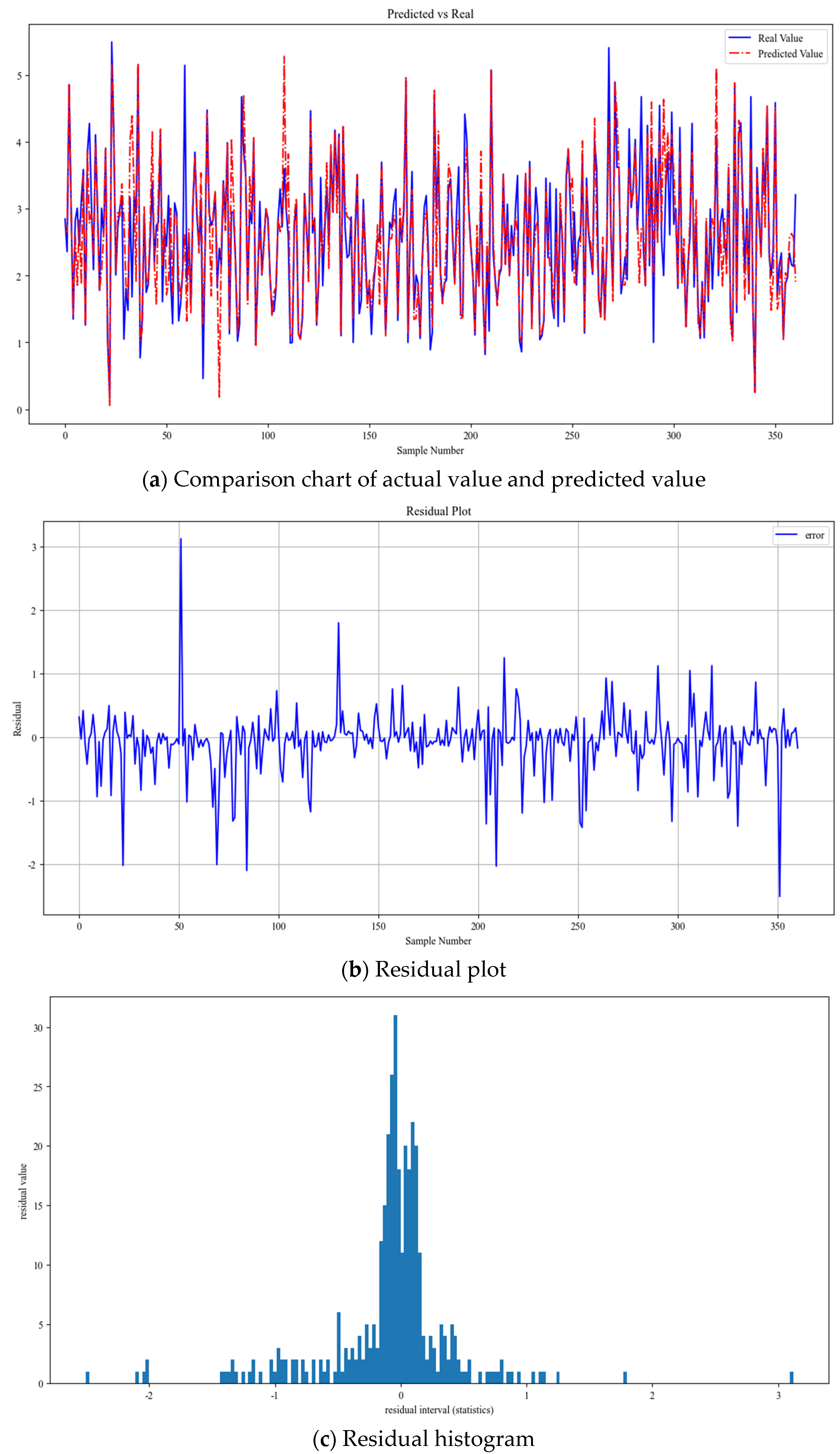
The mutual information method was used for feature selection, effectively extracting features highly related to yield. This optimized the model’s input and improved prediction accuracy and robustness. Compared with traditional methods, this approach significantly reduced feature dimensions and enhanced the model’s computational efficiency. Production capacity predictions were made using three machine learning models: XGBoost, random forest, and SVR, based on 11 contributing feature values. The R² values on the test set were 0.85, 0.83, and 0.77, respectively, indicating high prediction performance.

(3)

The SHAP value method was introduced to interpret the model, making the model’s output interpretable and enabling the clear identification of factors with the greatest impact on production. Compared with traditional black box models, this method provides more powerful guidance for engineering practice. According to the SHAP value results, the five factors of the starting time of wells, GLR, time to close the well, catcher well inclination angle, and shut-in tubing pressure were identified as the dominant factors affecting the gas production of plunger gas lift wells.

(4)

In future research, the feature selection method should be further studied and optimized, and more actual production data should be incorporated to enhance the scientificity and effectiveness of feature selection, thereby further improving the predictive ability and stability of the model. Additionally, the SHAP value method can be applied to other machine learning models to improve their interpretability, enabling the model to not only enhance prediction accuracy in practical applications, but also provide clear guidance for operations and decision-making. Moreover, it is necessary to compare more different types of machine learning models, evaluate their performance on various oil and gas field data sets, find the most suitable application scenario model, and improve the universality and wide applicability of the prediction.

(5)

In this numerical study, only the engineering factors and production factors of the wellbore part were considered, without obtaining the corresponding reservoir and other related data. Therefore, when this machine learning method is subsequently used for production prediction and influencing factor analysis, it is recommended that consideration be given to adding reservoir and other related information to make the prediction and influencing factor analysis of the model more complete.

References

1. Wenzhi, Z.; Ailin, J.; Yunsheng, W.; Junlei, W.; Hanqing, Z. Progress in shale gas exploration in China and prospects for future development. China Pet. Explor. 2020, 25, 31–44. [Google Scholar]
2. Caineng, Z.; Qun, Z.; Hongyan, W.; Qian, S.; Nan, S.; Zhiming, H.; Dexun, L. Theory and Technology of Unconventional Oil and Gas Exploration and Development Helps China Increase Oil and Gas Reserves and Production. Pet. Sci. Technol. Forum 2021, 40, 72–79. [Google Scholar]
3. National Energy Administration. China Natural Gas Development Report; Petroleum Industry Press: Beijing, China, 2023.
4. Bochun, L.; Jianhua, X.; Fan, X.; Linjuan, Z.; Kun, Z.; Mi, J.; Fan, Y. Large-Scale Application and Effect Analysis of Plunger Gas Lift Technology in Changning Shale Gas Reservoir. Drill. Prod. Technol. 2023, 46, 65–70. [Google Scholar]
5. Miao, J.; Niu, L. A survey on feature selection. Procedia Comput. Sci. 2016, 91, 919–926. [Google Scholar] [CrossRef]
6. Lea, J.F. Dynamic Analysis of Plunger Lift Operations. J. Pet. Technol. 1982, 34, 2617–2629. [Google Scholar] [CrossRef]
7. Gasbarri, S.; Wiggins, M.L. A Dynamic Plunger Lift Model for Gas Wells. SPE Prod. Fac. 2001, 16, 89–96. [Google Scholar] [CrossRef]
8. Ozkan, E.; Keefer, B.; Miller, M.G. Optimization of Plunger-Lift Performance in Liquid Loading Gas Wells. In Proceedings of the Canadian International Petroleum Conference, Denver, CO, USA, 5–8 October 2003. [Google Scholar] [CrossRef]
9. Ajay Singh Singh, A. Application of data mining for quick root-cause identification and automated production diagnostic of gas wells with plunger lift. SPE Prod. Oper. 2017, 32, 279–293. [Google Scholar]
10. Ranjan, A.; Verma, S.; Singh, Y. Gas lift optimization using artificial neural network. In SPE Middle East Oil & Gas Show and Conference; OnePetro: Richardson, TX, USA, 2015. [Google Scholar]
11. Nandola, N.N.; Kaisare, N.S.; Gupta, A. Online optimization for a plunger lift process in shale gas wells. Comput. Chem. Eng. 2018, 108, 89–97. [Google Scholar] [CrossRef]
12. Shi, J.; Chen, S.; Zhang, X.; Zhao, R.; Liu, Z.; Liu, M.; Zhang, N.; Sun, D. Artificial lift methods optimising and selecting based on big data analysis technology. In Proceedings of the International Petroleum Technology Conference, IPTC, Beijing, China, 26–28 March 2019; p. D011S010R003. [Google Scholar]
13. Ounsakul, T.; Sirirattanachatchawan, T.; Pattarachupong, W.; Yokrat, Y.; Ekkawong, P. Artificial lift selection using machine learning. In Proceedings of the International Petroleum Technology Conference, IPTC, Beijing, China, 26–28 March 2019; p. D021S042R003. [Google Scholar]
14. Chaodong, T.; Wenrong, S.; Loulou, L.; Peng, Q.; Zhaomin, G.; Wu, H. Research on Optimization Decision of Plunger Gas Lift Operation Based on Data Driven. In Proceedings of the 2019 IEEE Eurasia Conference on IOT, Communication and Engineering (ECICE), Yunlin, Taiwan, 3–6 October 2019; IEEE: Piscataway, NJ, USA, 2019; pp. 263–266. [Google Scholar]
15. Akhiiartdinov, A.; Pereyra, E.; Sarica, C.; Severino, J. Data Analytics Application for Conventional Plunger Lift Modeling and Optimization. In SPE Artificial Lift Conference and Exhibition—Americas; OnePetro: Richardson, TX, USA, 2020. [Google Scholar]
16. Sami, N.A. Application of machine learning algorithms to predict tubing pressure in intermittent gas lift wells. Pet. Res. 2022, 7, 246–252. [Google Scholar] [CrossRef]
17. Xie, Y.; Ma, S.; Wang, H.; Li, N.; Zhu, J.; Wang, J. Unsupervised clustering for the anomaly diagnosis of plunger lift operations. Geoenergy Sci. Eng. 2023, 231, 212305. [Google Scholar] [CrossRef]
18. Petch, J.; Di, S.; Nelson, W. Opening the black box: The promise and limitations of explainable machine learning in cardiology. Can. J. Cardiol. 2022, 38, 204–213. [Google Scholar] [CrossRef] [PubMed]
19. Narwaria, M. Does explainable machine learning uncover the black box in vision applications? Image Vis. Comput. 2022, 118, 104353. [Google Scholar] [CrossRef]
20. Aas, K.; Jullum, M.; Løland, A. Explaining individual predictions when features are dependent: More accurate approximations to Shapley values. Artif. Intell. 2021, 298, 103502. [Google Scholar] [CrossRef]
21. Lubo-Robles, D.; Devegowda, D.; Jayaram, V.; Bedle, H.; Marfurt, K.J.; Pranter, M.J. Machine learning model interpretability using SHAP values: Application to a seismic Facies classification task. In SEG Technical Program Expanded Abstracts 2020; Society of Exploration Geophysicists: Houston, TX, USA, 2020. [Google Scholar] [CrossRef]
22. Tran, N.L.; Gupta, I.; Devegowda, D.; Jayaram, V.; Karami, H.; Rai, C.; Sondergeld, C.H. Application of Interpretable Machine-Learning Workflows to Identify Brittle, Fracturable, and Producible Rock in Horizontal Wells Using Surface Drilling Data. SPE Reserv. Eval. Eng. 2020, 23, 1328–1342. [Google Scholar] [CrossRef]
23. Cross, T.; Sathaye, K.; Darnell, K.; Niederhut, D.; Crifasi, K. Predicting water production in the williston basin using a machine learning model. In Proceedings of the 8th Unconventional Resources Technology Conference, Virtual, 20–22 July 2020; American Association of Petroleum Geologists: Houston, TX, USA, 2020. [Google Scholar]
24. Ma, X.; Zhou, D.; Cai, W.; Li, X.; He, M. An Interpretable Machine Learning Approach to Prediction Horizontal Well Productivity. J. Southwest Pet. Univ. Sci. Technol. Ed. 2022, 44, 81–90. [Google Scholar] [CrossRef]
25. Lu, X.; Zhao, Y.; Peng, J. Analysis of Influencing Factors of Plunger Gas Lift Technology. Mech. Electr. Eng. Technol. 2022, 51, 141–144. [Google Scholar]
26. Kong, Q.; Ye, C.; Sun, Y. Research on data preprocessing methods for big data. Comput. Technol. Dev. 2018, 28, 1–4. [Google Scholar] [CrossRef]
27. Shannon, C.E. A mathematical theory of communication. SIGMOBILE Mob. Comput. Commun. Rev. 2001, 5, 3–55. [Google Scholar] [CrossRef]
28. Chen, T.; Guestrin, C. XGBoost: A scalable tree boosting system. In Proceedings of the 22nd ACM SIGKDD International Conference on Knowledge Discovery and Data Mining, San Francisco, CA, USA, 13–17 August 2016; pp. 785–794. [Google Scholar]
29. Shapley, L.S. Contributions to the Theory of Games (AM-28); Kuhn, H.W., Tucker, A.W., Eds.; Princeton University Press: Princeton, NJ, USA, 1953; pp. 307–318. [Google Scholar]
30. Saifulizan, S.S.B.H.; Busahmin, B.; Prasad, D.M.R.; Elmabrouk, S. Evaluation of Different Well Control Methods Concentrating on the Application of Conventional Drilling Technique. ARPN J. Eng. Appl. Sci. 2023, 18, 1851–1857. [Google Scholar]
31. Profillidis, V.A.; Botzoris, G.N. Econometric, Gravity, and the 4-Step Methods. In Modeling of Transport Demand; Elsevier: Amsterdam, The Netherlands, 2019; pp. 271–351. [Google Scholar] [CrossRef]
32. Li, Q.; Han, Y.; Liu, X.; Ansari, U.; Cheng, Y.; Yan, C. Hydrate as a by-product in CO2 leakage during the long-term sub-seabed sequestration and its role in preventing further leakage. Environ. Sci. Pollut. Res. 2022, 29, 77737–77754. [Google Scholar] [CrossRef]
33. Li, Q.; Wang, F.; Wang, Y.; Forson, K.; Cao, L.; Zhang, C.; Chen, J. Experimental investigation on the high-pressure sand suspension and adsorption capacity of guar gum fracturing fluid in low-permeability shale reservoirs: Factor analysis and mechanism disclosure. Environ. Sci. Pollut. Res. 2022, 29, 53050–53062. [Google Scholar] [CrossRef] [PubMed]
Figure 1. Workflow diagram.
Processes 12 01888 g001
Figure 2. Entropy diagram.
Processes 12 01888 g002
Figure 3. Mutual information diagram.
Processes 12 01888 g003
Figure 4. Sixfold cross-validation schematic diagram.
Processes 12 01888 g004
Figure 5. Proportion of missing data values.
Processes 12 01888 g005
Figure 6. Histogram of characteristic data and gas production.
Processes 12 01888 g006aProcesses 12 01888 g006b
Figure 7. Pearson correlation heatmap.
Processes 12 01888 g007
Figure 8. Mutual information values of 11 gas production values relative to plunger gas lift wells.
Processes 12 01888 g008
Figure 9. Prediction graph and error statistics graph of XGBoost model.
Processes 12 01888 g009
Figure 10. Prediction graph and error statistics graph of random forest model.
Processes 12 01888 g010
Figure 11. Prediction graph and error statistics graph of SVR model.
Processes 12 01888 g011
Figure 12. XGBoost model SHAP value global interpretation.
Processes 12 01888 g012
Figure 13. XGBoost model SHAP value local interpretation.
Processes 12 01888 g013
Figure 14. Global interpretation of SHAP values of Random Forest model.
Processes 12 01888 g014
Figure 15. Local interpretation of SHAP values of random forest model.
Processes 12 01888 g015