Reservoir Porosity Construction Based on BiTCN-BiLSTM-AM Optimized by Improved Sparrow Search Algorithm

Abstract

To evaluate reservoir porosity accurately, a method based on the bidirectional temporal convolutional network (BiTCN), bidirectional long short-term memory network (BiLSTM), and attention mechanism (AM) optimized by the improved sparrow search algorithm (ISSA) is proposed. Firstly, the sparrow search algorithm improved by a phased control step size strategy and dynamic random Cauchy mutation is introduced. Secondly, the superiority of the ISSA is confirmed by the test functions of Congress on Evolutionary Computation in 2022 (CEC-2022). Furthermore, the experimental findings are assessed using the Wilcoxon test, which provides additional evidence of the ISSA’s superiority against the competing algorithms. Finally, the BiTCN-BiLSTM-AM is optimized by the ISSA, and the ISSA-BiTCN-BiLSTM-AM was applied to reservoir porosity construction in the Midlands basin. The results showed that the RMSE and MAE of the proposed model were 0.4293 and 0.5696, respectively, which verified the effectiveness and success rate of reservoir parameter construction by addressing the shortcomings in the capabilities shown by conventional interpretation procedures.

1. Introduction

Logging is an essential method to identify the characteristics of subsurface rocks and fluids using devices that monitor physical information [1]. Nevertheless, because logging and coring only provide a small amount of reservoir information, the assessment of reservoir parameters is inadequate. To calculate the reservoir parameters effectively, the empirical formula or simplified geologic model are constructed. However, this prediction is not very good due to the very heterogeneous reservoirs [2]. The amount of logging data is increasing exponentially, reaching a significant volume and exhibiting traits like mass, multiple-scale, and constant shifting. Because of the extreme heterogeneity of today’s petroleum reservoirs and the abundance of wells, a vast amount of diverse logging data is available. The abundance of geological information contained in these logging data can be successfully mined for valuable information that is needed to identify petroleum reserves [3].

Conventional logging interpretation techniques are very taxing. Recently, machine learning has drawn a lot of attention for the ability to solve intricate pattern recognition problems. Its benefits include great portability, robust learning capacity, and coverage of a high data-driven ceiling. Machine learning techniques have been widely used by researchers to solve a range of logging-related problems, such as calculating reservoir parameters [4], acquiring chromatographic information [5], and resolving the issue of missing logging data [6]. The foundation of the temporal convolutional network (TCN) is a methodical assessment of general convolutional and recursive structures intended for sequence modeling. It is regarded as a foundational approach for implementing deep networks on sequences. Nonetheless, the unidirectional TCN fails to consider the impact of prior knowledge on the outcome of prediction, resulting in inadequate feature extraction from logging data. The bidirectional temporal convolutional network (BiTCN) can be utilized to get around this restriction and improve feature extraction performance by combining both forward and backward information [7]. Recursive neural networks (RNNs) are designed for learning tasks that need to process sequential information [8]. However, the question of disappearance or diffusion of gradients has troubled its use. The long short-term memory network (LSTM) significantly reduces the training issues of RNNs by utilizing memory states and gating units. Nevertheless, the correlation of logging data information can only be utilized by the LSTM in a single direction. The constraint that the states of the LSTM propagate in a single way from back to front is addressed by the proposal of the BiLSTM [9,10]. It works well for activities in which the current moment’s output is connected to both the past and the future states. The attention mechanism (AM) is initially postulated in the domain of visual images [11]. It is noted that the AM can be used to maximize the conventional visual search technique [12]. The integration of the AM with a deep network enables the selective processing of data by determining how each piece of information contributes to the prediction goal.

The earlier section summarizes the BiTCN, BiLSTM, and AM. The constraints of the standard logging models in interpreting large and complex logging data are addressed in this study by proposing a hybrid deep learning model called the BiTCN-BiLSTM-AM, which primarily takes advantage of the BiTCN, BiLSTM, and AM’s benefits in handling time-series information. Temporal information in features can be effectively extracted by the BiTCN. The contextual relationship between the features can be obtained by the BiLSTM. To more accurately depict the distant relationships between features, the AM is offered. Additionally, the prediction performance can be considerably enhanced by optimizing the BiTCN-BiLSTM-AM using the improved sparrow search algorithm (ISSA).

The following is a summary of the principal contributions:

The BiTCN is applied to extract the implied relationship between input and output features, and the resulting data are then fed into the BiLSTM for prediction. Then, the AM is employed to enhance the impact of significant data on the BiLSTM output to further improve the prediction accuracy.

The phased control step size strategy and dynamic random Cauchy mutation are introduced to improve the SSA’s optimization capability. The prediction performance is enhanced by optimizing the BiTCN-BiLSTM-AM’s hyperparameters using the ISSA.

The ISSA-BiTCN-BiLSTM-AM considerably surpasses the rival models in complex reservoir parameter construction in engineering practice, can effectively address the needs of the actual industry, and has practical ramifications.

2. Principle and Modeling

2.1. Principle of the BiTCN-BiLSTM-AM

2.1.1. BiTCN

The TCN is made up of identical input and output length dilated causal convolutional layers. However, the TCN ignores the implicit back information and can just extract the forward features. To better acquire the long-time dependence of logging data, the BiTCN is employed to capture the hidden characteristics both forward and backward. Figure 1 depicts the bidirectional dilated causal convolutional network.

Causal convolution relies on the principles of time series to presume that the output information depends on the backward input. Causal convolution needs more layers or a broader receptive field to capture long-time properties. The BiTCN uses dilated convolution, which preserves the dimensionality of feature mapping while achieving a bigger receptive field with fewer layers.

When the input time series is $X=(x_1,x_2,\dots , x_T), X\in R^n$ and the filter is $F=(f_1, f_2,\dots , f_k)$, the output of $x_T$ after dilated convolution is expressed by Equation (1):

$$Y(T)=\sum _{i=0}^{k-1}F\left(i\right)·x_{T-d·i}$$

(1)

where $k$ is the filter size, and $T-d·i$ is the backward direction. The dilation factor $d$ controls the number of zero vectors put in between two convolution kernels that are next to each other. The factor $d$ increases rapidly after every layer of the input series’ convolution. A bigger receptive field is obtained by the BiTCN. However, issues like gradient disappearance and sluggish convergence arise when the BiTCN’s receptive field is expanded. To avoid these issues, the residual module is introduced, which is shown in Figure 2.

2.1.2. BiLSTM

The LSTM is a classical model with nodes including the forget gates, output gates, and input gates. The LSTM can avoid the problem of vanishing gradients and perform admirably in situations where long-term linkages between input and output are needed. The idea of the BiLSTM addresses the restriction that the states of the LSTM propagate in a single direction from back to front. It functions well for tasks where the output of the present is related to both the past and future. In the BiLSTM, the final output is generated by combining the forward and backward hidden outputs.

The structure of the BiLSTM is displayed in Figure 3.

The attention mechanism (AM) amplifies the impact of significant data on the prediction outcomes by using training weights to provide varying weights to the input data. The weight of the attention layer can be calculated by Equations (2)–(4):

$$e_t=utanh\left(w{h}_t\right)$$

(2)

$${\alpha }_t={\displaystyle \frac{\mathrm{e}\mathrm{x}\mathrm{p}\left(e_t\right)}{{\sum }_{j=1}^t{e}_j}}$$

(3)

$$y_{attention}=\sum _{t=1}^i{\alpha }_t{h}_t$$

(4)

where $e_t$ is the attention probability distribution; $u$ and $w$ are the weights; $y_{attention}$ is the final output; $x_t$ is the input of the BiLSTM; $h_t$ is the output of the hidden layer; and ${\alpha }_t$ is the attention probability distribution.

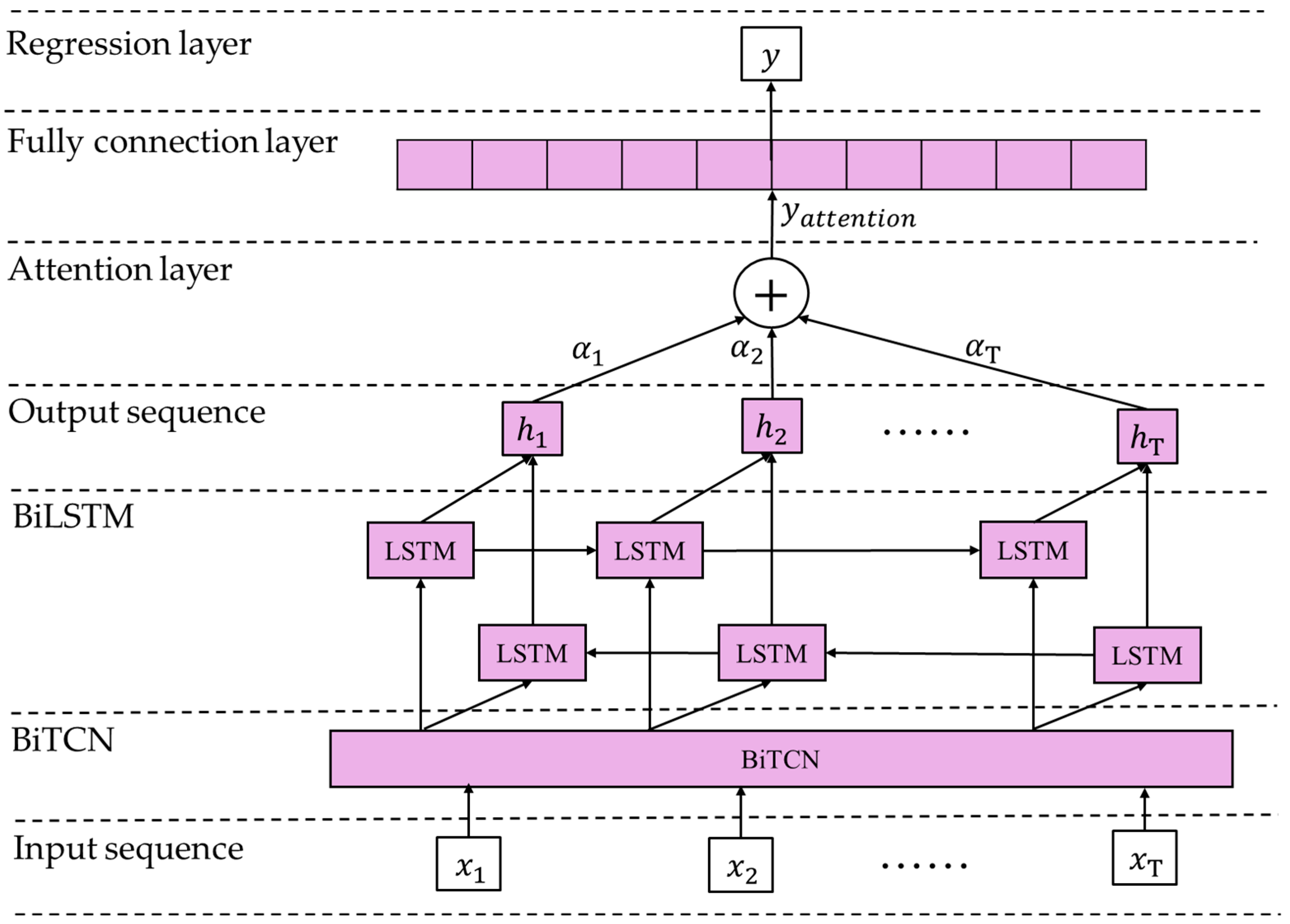
2.1.3. BiTCN-BiLSTM-AM

The structure of the BiTCN-BiLSTM-AM is shown in Figure 4. The whole structure is composed of six parts including the input, BiTCN, BiLSTM, AM, full connection, and output.

2.2. Principle of the SSA

The sparrow search algorithm (SSA) is inspired by the group wisdom, foraging, and anti-predation behaviors of sparrows [13].

The producer’s position can be calculated by Equation (5):

$$x_{i,j}^{t+1}=\left\{\begin{array}{c}{x}_{i,j}^t·\mathit{exp}\left({\displaystyle \frac{-i}{\alpha ·{iter}_{max}}}\right), R_2<S_T\\ x_{i,j}^t+Q·L, R_2\ge S_T\end{array}\right.$$

(5)

where $x_{i,j}^t$ is the $j$th dimensional position of the $i$th individual in the $t$th iteration; ${iter}_{max}$ is the maximum value of the iterations; $\alpha$ is a random value in $[0, 1]$; $Q$ is a random value with the normal distribution; $L$ is a $1\times d$ matrix where each value is 1; $S_T$ is the alert threshold in $[0.5, 1]$; and $R_2$ is the warning value in $[0, 1]$.

When $R_2<S_T$, which indicates that there are no predators around, the producer switches to the extended hunt mode. $R_2\ge S_T$ indicates that some sparrows have spotted the predator. If this is the case, all sparrows need to take off right away for safer locations.

Scroungers follow producers who can provide the best food. Some may compete for food while keeping a watchful eye on the producers. The scrounger’s position can be calculated by Equation (6):

$$x_{i,j}^{t+1}=\left\{\begin{array}{c}Q·\mathit{exp}\left({\displaystyle \frac{x_{worst}^t-x_{i,j}^t}{i^2}}\right), i>n/2\\ x_p^{t+1}+\left|x_{i,j}^t-x_p^{t+1}\right|·A^{+}·L, i\le n/2\end{array}\right.$$

(6)

where $x_{worst}^t$ is the current global worst location; $x_p^{t+1}$ is the optimal position; $A^{+}=A^T{\left({AA}^T\right)}^{-1}$, where $A$ is a $1\times d$ matrix where each element is randomly assigned 1 or −1; $n$ is the size of the sparrow population; and $i>n/2$ indicates that the $i$th scrounger with the worse fitness is probably famished.

When a threat is detected, the sparrows around the group’s edge quickly go toward the safe area to take up a better position, while the sparrows in the group’s core flit around aimlessly to remain near to one another. The model can be calculated by Equation (7):

$$x_{i,j}^{t+1}=\left\{\begin{array}{c}{x}_{best}^t+\beta ·\left|x_{i,j}^t-x_{best}^t\right|, f_i>f_g\\ x_{i,j}^t+K·\left({\displaystyle \frac{\left|x_{i,j}^t-x_{worst}^t\right|}{\left(f_i> f_w\right)+\epsilon }}\right), f_i=f_g\end{array}\right.$$

(7)

where $x_{best}$ is the current global optimal position; $\beta$ is a random value with normal distribution; $K$ is a random value in $[-1, 1]$; $f_i$ is the present fitness value; $f_g$ and $f_w$ represent the global best and worst fitness values, respectively; $\epsilon$ is the tiniest constant to eliminate the case of zero-division error; $f_i>f_g$ indicates that a sparrow is at the group’s periphery; and $f_i=f_g$ indicates that the sparrows in the middle are aware of the threat and should get closer to each other.

2.3. Improvement of the SSA

2.3.1. Phased Control Step Size Strategy

In the SSA, there is no effective control of step size. When $R_2<S_T$, the producer adopts a spiral search strategy, which brings the problem of insufficient search accuracy. Therefore, the nonlinear attenuation factor $u$ is introduced search widely in different regions in the early stage, and focus on developing known regions in the middle and late stages, so as to improve the search accuracy and convergence speed.

The producer’s position can be calculated by Equations (8)–(11):

$$x_{i,j}^{t+1}=\left\{\begin{array}{c}{x}_{best}^t+\beta ·\left|x_{i,j}^t-x_{best}^t\right|·e^l·cos\left(2\pi l\right), R_2<0.5\\ x_{i,j}^t·\mu , {0.5\le R}_2<\acute{S_T}\\ x_{i,j}^t+Q, R_2\ge \acute{S_T}\end{array}\right.$$

(8)

$$l=(\alpha -1)·rand+1$$

(9)

$$\alpha =(-{\displaystyle \frac{t}{{iter}_{max}}})-1$$

(10)

$$\mu ={\displaystyle \frac{1}{e^{w·\frac{t}{{iter}_{max}}}}}$$

(11)

where $\acute{S_T}\in [0.8, 1]$ is the safe value; $rand$ is a random value in $[0, 1]$; $w$ is a constant, which can be taken to be 5.5; and $\mu$ is the attenuation factor.

In the process of iterative updating, the attenuation factor $\mu$ has a larger weight in the early stage and a faster change rate, and the producer can keep exploring the unknown region to avoid premature convergence in the early stage. In the later iterations, the weight of the attenuation factor $\mu$ is small and the change rate is slow, so the producer can maintain strong local development ability, narrow the search scope, and accelerate the algorithm convergence.

2.3.2. Dynamic Random Cauchy Mutation

The Cauchy mutation has a better disturbance ability than the Gaussian distribution because it has a smoother trend and a lower peak value at the far point. The introduction of the Cauchy mutation in the updating process can significantly improve the global optimization ability. To synthetically balance the global search ability of the algorithm in the early stage and the convergence ability in the later stage, the dynamic mutation probability $P_e$ defined. The specific process of the dynamic random Cauchy mutation is as follows:

(1) Calculate the contemporary mutation probability $P_e$, which is calculated by the Equation (12):

$$P_e={(1-{\displaystyle \frac{t}{iter}})}^{10}+\epsilon$$

(12)

where $\epsilon$ is the adjustment parameter, which can be set as 0.06, and $iter$ is the maximum iterations.

(2) The individual is randomly selected for Cauchy variation according to Equation (13):

$$X^{t+1}=X^t\left(1+tan\left(\pi \right(\mu -0.5\left)\right)\right)$$

(13)

where $X^t$ and $X^{t+1}$ are the individuals’ positions before and after Cauchy mutation, respectively, and $\mu$ is a random value between 0 and 1.

(3) The greedy rule is introduced to compare the individual fitness before and after mutation to determine whether to perform the mutation operation. The greed rules are calculated by Equation (14):

$$X_{best}=\left\{\begin{array}{c}{X}^{t+1}, f\left(X^{t+1}\right)<f\left(X_{best}\right)\\ X_{best},f\left(X^{t+1}\right)\ge f\left(X_{best}\right)\end{array}\right.$$

(14)

By employing the Cauchy mutation to disturb individuals in the sparrows’ position updating, the SSA’s search scope is increased and its capacity to break out of the local optimum is enhanced. As a result, the dynamic random Cauchy mutation can take the place of the original scroungers’ position update formula.

2.3.3. ISSA Calculation Flow

The outline of the fundamental steps of the ISSA is shown in Algorithm 1.

Algorithm 1: The framework of the ISSA.

Input:

$G$: the maximum iterations

$PD$: the quantity of producers

$SD$: the quantity of sparrows sensing danger

$R2$: the alarm value

$n$: the quantity of sparrows

Initialize the population and define the relevant parameters.

Output:$X_{best}$, $f_g$.

1: while ($t<G$)

2: Determine which is currently the best and worst fit by ranking the fitness values.

3: $R2=rand\left(1\right)$

4: for $i=1 : PD$

5:  Update the position with Equations (8)–(11);

6: end for

7: for $i=(PD+1) : n$

8:  Update the position with Equations (12)–(14);

9: end for

10: for $i=1 : SD$

11:  Update the position with Equation (7);

12: end for

13: Get the current position;

14: Update if the new position is better.

15: $t=t+1$

16: end while

17: return $X_{best}$, $f_g$

3. ISSA Performance Test

In this section, CEC-2022 functions are used to test the performance of the ISSA and the rival algorithms including the SSA [13], pelican optimization algorithm (POA) [14], dung beetle optimizer (DBO) [15], and whale optimization algorithm (WOA) [16].

3.1. Analysis of Convergence Curves

The convergence curves for the ISSA and other algorithms on CEC-2022 functions are shown in Figure 5. The quantitative results are shown in

Table 1. Results of the ISSA and the rival algorithms on CEC-2022 functions. The best are bolded, and the standard deviations are shown in parentheses.

Function	ISSA	SSA	POA	DBO	WOA
F1	3.12 × 102	2.21 × 103	8.75 × 102	6.83 × 103	1.12 × 103
	(5.17 × 100)	(1.59 × 103)	(8.89 × 102)	(2.87 × 103)	(6.34 × 102)
F2	4.23 × 102	4.31 × 102	4.29 × 102	4.64 × 102	4.59 × 102
	(3.15 × 101)	(2.51 × 101)	(3.19 × 101)	(3.28 × 101)	(7.27 × 101)
F3	6.14 × 102	6.20 × 102	6.27 × 102	6.26 × 102	6.46 × 102
	(7.39 × 100)	(1.09 × 101)	(1.07 × 101)	(1.12 × 101)	(1.01 × 101)
F4	8.12 × 102	8.28 × 102	8.21 × 102	8.48 × 102	8.33 × 102
	(5.06 × 100)	(6.17 × 100)	(6.88 × 100)	(8.74 × 100)	(9.88 × 100)
F5	1.16 × 103	1.14 × 103	1.10 × 103	1.02 × 103	1.48 × 103
	(2.61 × 102)	(1.83 × 102)	(1.33 × 102)	(1.09 × 102)	(1.86 × 102)
F6	3.51 × 103	4.48 × 103	3.76 × 103	4.95 × 104	6.63 × 103
	(2.08 × 103)	(2.16 × 103)	(2.38 × 103)	(2.72 × 104)	(4.62 × 103)
F7	2.01 × 103	2.06 × 103	2.04 × 103	2.10 × 103	2.09 × 103
	(1.91 × 101)	(2.84 × 101)	(1.09 × 101)	(4.14 × 101)	(3.39 × 101)
F8	2.20 × 103	2.20 × 103	2.20 × 103	2.24 × 103	2.21 × 103
	(2.86 × 100)	(3.47 × 100)	(1.94 × 101)	(2.39 × 101)	(1.02 × 101)
F9	2.51 × 103	2.52 × 103	2.52 × 103	2.65 × 103	2.62 × 103
	(5.04 × 100)	(3.27 × 101)	(2.09 × 101)	(4.45 × 101)	(4.84 × 101)
F10	2.54 × 103	2.56 × 103	2.51 × 103	2.55 × 103	2.56 × 103
	(6.98 × 101)	(6.89 × 101)	(5.76 × 101)	(1.82 × 102)	(1.31 × 102)
F11	2.71 × 103	2.88 × 103	2.76 × 103	3.15 × 103	2.72 × 103
	(1.15 × 102)	(2.09 × 102)	(1.78 × 102)	(2.40 × 102)	(1.10 × 102)
F12	2.81 × 103	2.85 × 103	2.84 × 103	2.85 × 103	2.89 × 103
	(2.47 × 100)	(1.71 × 101)	(1.30 × 101)	(1.27 × 101)	(5.00 × 101)

. It can be found that the ISSA has a faster convergence rate and a smaller average fitness value.

3.2. Statistical Analysis of ISSA

To make further comparisons, the Wilcoxon test is applied to determine whether the ISSA has a significant performance difference when compared to the rival algorithms at a significance threshold of 5% confidence. Additionally, each algorithm’s ranking is established by the Friedman test.

The results of the Wilcoxon test are shown in

Table 2. Pairwise comparison of the ISSA and the rival algorithms. When $p<0.05$, the ISSA is superior; when $p>0.05$, the ISSA is inferior.

Function	ISSA vs. SSA		ISSA vs. POA		ISSA vs. DBO		ISSA vs. WOA
	p	h	p	h	p	h	p	h
F1	3.13 × 10−11	+	3.13 × 10−11	+	3.13 × 10−11	+	3.13 × 10−11	+
F2	3.52 × 10−2	+	3.13 × 10−2	+	8.14 × 10−5	+	1.98 × 10−2	+
F3	2.02 × 10−7	+	1.71 × 10−8	+	3.34 × 10−8	+	4.51 × 10−11	+
F4	4.72 × 10−4	+	1.81 × 10−4	+	2.16 × 10−7	+	6.14 × 10−4	+
F5	4.56 × 10−1	−	9.48 × 10−1	−	5.47 × 10−1	−	5.94 × 10−5	+
F6	2.70 × 10−2	+	7.50 × 10−2	+	3.02 × 10−11	+	3.75 × 10−4	+
F7	3.31 × 10−6	+	1.19 × 10−2	+	8.09 × 10−10	+	2.46 × 10−9	+
F8	7.08 × 10−8	+	2.61 × 10−3	+	6.68 × 10−11	+	2.16 × 10−8	+
F9	2.03 × 10−10	+	2.29 × 10−6	+	2.30 × 10−11	+	3.39 × 10−11	+
F10	3.46 × 10−1	−	8.41 × 10−1	−	7.59 × 10−7	+	4.92 × 10−5	+
F11	8.89 × 10−6	+	1.66 × 10−2	+	5.36 × 10−11	+	4.34 × 10−6	+
F12	4.05 × 10−2	+	4.80 × 10−2	+	3.62 × 10−8	+	3.17 × 10−10	+

. The ISSA is significantly different from the rival algorithms in the functions F1–F4, F6–F9, and F11–F12. For F5, the ISSA is similar to the SSA, POA, and DBO. For F10, the ISSA is similar to the SSA and POA.

The results of the Friedman test are shown in

Table 3. Results of the Friedman test.

Friedman Test	ISSA	SSA	POA	DBO	WOA
Mean	2.4112	3.1431	4.5624	4.0432	7.0856
Rank	1	2	4	3	5

. The mean ranking value (Mean) of the ISSA is 2.4112, which is lower than the rival algorithms. It can be seen that the ISSA’s optimization ability is superior to the rival algorithms on the whole.

4. Practical Application and Result Analysis

4.1. ISSA-BiTCN-BiLSTM-AM Prediction Flow

It is challenging to create the ideal model in traditional model training since parameter selection is done by hand based on experience, which is heavily influenced by subjective considerations. Therefore, the ISSA can be applied to find the ideal parameters of the BiTCN-BiLSTM-AM, including the number of nodes in the hidden layer, initial learning rate, and L2 regularization coefficient.

The specific steps of the ISSA-BiTCN-BiLSTM-AM are as follows:

Step 1: Divide the input data set into the training set and test set. Additionally, the Kolmogorov-Smirnov Two-Sample Test is used to compare whether two samples come from the same continuous distribution. Then, the data set is normalized to [0, 1] using the max-min normalization method.

Step 2: Establish an objective function model. The objective function is the root mean square error (RMSE), which is expressed as in Equation (15):

$$\mathrm{R}\mathrm{M}\mathrm{S}\mathrm{E}=\sqrt{{\displaystyle \frac{1}{N}}{\sum }_{i=1}^N{\left(y_k-{\widehat{y}}_k\right)}^2}$$

(15)

where $y_k$ and ${\widehat{y}}_k$ are the true value and predicted value, respectively.

Step 3: The ISSA is used to optimize the parameters in the BiTCN-BiLSTM-AM under the cross-validation.

Step 4: Apply the BiTCN-BiLSTM-AM with the optimal parameters to the estimation.

4.2. Data Preparation

It is challenging to quantify porosity in complicated lithologies with traditional well logging. Since NMR-derived porosity is determined without taking into account mineralogy and matrix, it is regarded as the “gold standard” for total porosity. Unfortunately, most wells lack these data since NMR techniques are still relatively new technology and because they incur additional costs for logging runs and rig time. To reduce inaccuracy in petrophysical models, the ability to reliably predict NMR-derived porosity using conventional logs is very valuable. The data set of well A used to model for NMR-derived porosity is from the Haliburton MRIL logging drilled by Devon Energy in the Midlands basin. Additionally, the interest interval is the Wolfcamp formation (2140–2300 m). Figure 6 displays the logging graph.

4.3. Analysis of Forecast Results

The data set in well A at depths ranging from 2140 to 2260 m is used as the training data set and the rest is used as the validation data set. Additionally, the data sets in the training and validation parts have passed the Kolmogorov-Smirnov test. This ensures that they come from the same continuous distribution. The training data set can be utilized to train the ISSA-BiTCN-BiLSTM-AM and rival models (BPNN, BiTCN, and BiLSTM) under five-fold cross-validation. The input parameters are the following: DT, RT, GR, NPHI, DEPTH, and CAL. The output parameter is NMR porosity.

The search range of the parameters needed to be optimized by the ISSA is restricted to avoid a large search space impacting optimization efficiency. In particular, there is a 10 to 100 limit on the number of nodes in the hidden layer, a 10⁻⁴ to 10⁻³ limit on the initial learning rate, and a 10⁻⁸ to 10⁻² limit on the L2 regularization coefficient. Figure 7 displays the fitness decline rate during the BiTCN-BiLSTM-AM training phase. It is evident that the ISSA converges faster than the rival algorithms and that its ultimate error is smaller than that of rival algorithms.

The parameter optimization results of the ISSA are as follows: the number of nodes in the hidden layer is 58, the initial learning rate is 0.0021, and the L2 regularization coefficient is 0.0029. The “missing” porosity of well A at depths between 2260 and 2300 m can be anticipated by the trained model.

Table 4. Quantitative results of prediction in well A at depths ranging from 2260 to 2330 m.

Models	MAE	RMSE
BPNN	1.1327	1.0658
BiTCN	0.8712	0.8925
BiLSTM	0.7661	0.6981
ISSA-BiTCN-BiLSTM-AM	0.5696	0.4293

displays the rival models’ and ISSA-BiTCN-BiLSTM-AM’s quantitative prediction results. The least successful model is the BPNN. It can be inferred that a model based on time series is superior to an ordinary model for the porosity prediction scenario. The most effective model is the ISSA-BiTCN-BiLSTM-AM. This is because it uses the BiTCN-BiLSTM-AM to process the time series features and applies the ISSA to acquire the optimal weights.

Figure 8 displays the contrast of the trained models’ estimated porosity and NMR porosity for well A at depths ranging from 2260 to 2300 m. The ISSA-BiTCN-BiLSTM-AM‘s prediction results match the measured porosity better than the competing models. It can be demonstrated that the ISSA-BiTCN-BiLSTM-AM is more successful at reservoir parameter construction.

5. Conclusions

A combined model named the ISSA-BiTCN-BiLSTM-AM is proposed for reservoir porosity construction. The following three conclusions can be drawn:

(1) The ISSA reduces the tendency to settle into the local optimal region during the search process and increases search efficiency with its phased control step size strategy and dynamic random Cauchy mutation.

(2) The BiTCN-BiLSTM-AM integrates the network structure of the BiTCN, BiLSTM and AM. In addition to handling complicated time dependencies, this hybrid design enhances the processing flexibility for time series’ dynamic features.

(3) The ISSA can improve prediction performance by fine-tuning the model’s hyperparameters. By optimizing the relevant parameters, overfitting of the model is effectively prevented and the generalization ability of the model is increased. The ISSA-BiTCN-BiLSTM-AM predictive model performs better than the rival models.

To summarize, the performance of the ISSA-BiTCN-BiLSTM-AM is outstanding. It can satisfy real-world engineering requirements. However, the ISSA-BiTCN-BiLSTM-AM has limitations that make it difficult to execute on mobile terminal devices, including high model complexity and large model size due to the large number of components. Upcoming research will focus on highly accurate lightweight networks.

References

1. Wang, P.; Peng, S. A New Scheme to Improve the Performance of Artificial Intelligence Techniques for Estimating Total Organic Carbon from Well Logs. Energies 2018, 11, 747. [Google Scholar] [CrossRef]
2. Nikolaos, C.K.; Athanassios, C.M.; Michail, C. The Contribution of Virtual Reality in Awareness and Preparedness of Oil and Gas Professionals. J. Eng. Sci. Technol. Rev. 2022, 15, 9–12. [Google Scholar]
3. Kok, M.V.; Gokcal, B.; Ersoy, G. Reservoir Analysis by Well Log Data. Energy Sources 2005, 27, 399–404. [Google Scholar] [CrossRef]
4. Yang, W.; Xia, K.W.; Fan, S. Oil Logging Reservoir Recognition Based on TCN and SA-BiLSTM Deep Learning Method. Eng. Appl. Artif. Intell. 2023, 121, 105950. [Google Scholar] [CrossRef]
5. Vaferi, B.; Eslamloueyan, R.; Ayatollahi, S. Automatic recognition of oil reservoir models from well testing data by using multi-layer perceptron networks. J. Pet. Sci. Eng. 2011, 77, 254–262. [Google Scholar] [CrossRef]
6. Geng, Z.; Hu, X.; Ding, N.; Zhao, S.; Han, Y. A pattern recognition modeling approach based on the intelligent ensemble classifier: Application to identification and appraisal of water-flooded layers. Proc. Inst. Mech. Eng. 2019, 233, 737–750. [Google Scholar] [CrossRef]
7. Zhang, D.; Chen, B.; Zhu, H.; Goh, H.H.; Dong, Y.; Wu, T. Short-term wind power prediction based on two-layer decomposition and BiTCN-BiLSTM-attention model. Energy 2023, 285, 128762. [Google Scholar] [CrossRef]
8. Hochreiter, S.; Schmidhuber, J. Long short-term memory. Neural Comput. 1997, 9, 1735–1780. [Google Scholar] [CrossRef] [PubMed]
9. Wang, Y.; Jia, P.; Peng, X. BinVulDet: Detecting vulnerability in binary program via decompiled pseudo code and BiLSTM-attention. Comput. Secur. 2023, 125, 103023. [Google Scholar] [CrossRef]
10. Wang, G.; Teng, H.; Qiao, L.; Yu, H.; Cui, Y.; Xiao, K. Well Logging Reconstruction Based on a Temporal Convolutional Network and Bidirectional Gated Recurrent Unit Network with Attention Mechanism Optimized by Improved Sand Cat Swarm Optimization. Energies 2024, 17, 2710. [Google Scholar] [CrossRef]
11. Zhang, C.; Chen, P.; Jiang, F.; Xie, J.; Yu, T. Fault Diagnosis of Nuclear Power Plant Based on Sparrow Search Algorithm Optimized CNN-LSTM Neural Network. Energies 2023, 16, 2934. [Google Scholar] [CrossRef]
12. Qiao, L.; He, N.; Cui, Y.; Zhu, J.; Xiao, K. Reservoir Porosity Prediction Based on BiLSTM-AM Optimized by Improved Pelican Optimization Algorithm. Energies 2024, 17, 1479. [Google Scholar] [CrossRef]
13. Awadallah, M.A.; Al-Betar, M.A.; Doush, I.A. Recent Versions and Applications of Sparrow Search Algorithm. Arch. Comput. Methods Eng. 2023, 30, 2831–2858. [Google Scholar] [CrossRef] [PubMed]
14. Xue, J.; Shen, B. Dung beetle optimizer: A new meta-heuristic algorithm for global optimization. J. Supercomput. 2022, 79, 7305–7336. [Google Scholar] [CrossRef]
15. Trojovsk, P.; Dehghani, M. Pelican Optimization Algorithm: A Novel Nature-Inspired Algorithm for Engineering Applications. Sensors 2022, 22, 855. [Google Scholar] [CrossRef] [PubMed]
16. Seyedali, M.; Andrew, L. The Whale Optimization Algorithm. Adv. Eng. Softw. 2016, 95, 51–67. [Google Scholar]
Figure 1. Structure of the bidirectional dilated causal convolutional network.
Processes 12 01907 g001
Figure 2. Structure of the residual module in the BiTCN.
Processes 12 01907 g002
Figure 3. Structure of the BiLSTM.
Processes 12 01907 g003
Figure 4. Structure of the BiTCN-BiLSTM-AM.
Processes 12 01907 g004
Figure 5. Convergence curves of the ISSA and the rival algorithms.
Processes 12 01907 g005
Figure 6. Logging graph of well A at depths ranging from 2140 to 2300 m.
Processes 12 01907 g006
Figure 7. Fitness reduction rate for training the BiTCN-BiLSTM-AM.
Processes 12 01907 g007
Figure 8. Logging graph showing the estimated and measured porosity in well A at depths ranging from 2260 to 2300 m.
Processes 12 01907 g008