Monitoring and Predicting Air Quality with IoT Devices

Abstract

The growing concern about air quality and its influence on human health has prompted the development of sophisticated monitoring and forecast systems. This article gives a thorough investigation into forecasting the air quality index (AQI) with an Internet of Things (IoT) device that analyzes temperature, humidity, PM10, and PM2.5 levels. The dataset used for this analysis comprises 5869 data points across six critical parameters essential for accurate air quality prediction. The data from these sensors is sent to the ThingSpeak cloud platform for storage and preliminary analysis. The system forecasts AQI using a TensorFlow-based regression model, delivering real-time insights. The combination of IoT technology and machine learning improves the accuracy and responsiveness of air quality monitoring systems, making it a useful tool for environmental management and public health protection. This work presents comparatively the effectiveness of feedforward neural network models trained with the ‘adam’ and ‘RMSprop’ optimizers over different epochs, as well as the machine learning algorithm random forest with varying numbers of estimators to forecast AQI. The models were trained using both types of regression analysis: linear regression and random forest regression. The findings show that the model achieves a high degree of accuracy, with the predictions closely aligning with the actual AQI values, thus having the potential to significantly reduce the negative health impact associated with poor air quality, protecting public health and alerting users when pollution levels are higher than allowed. Specifically, the random forest model with 100 estimators delivers the best overall performance for both AQI 10 and AQI 2.5, achieving the lowest Mean Absolute Error (MAE) of 0.2785 for AQI 10 and 0.2483 for AQI 2.5. This integration of IoT technology and advanced predictive analysis addresses the significant worldwide issue of air pollution by identifying the pollution hotspots and allowing decision-makers for quick reactions, and the development of effective strategies to reduce pollution sources.

1. Introduction

Due to permanent degradation, environmental monitoring is mandatory both for industrial companies and for society to keep life parameters in a normal range. Ecological monitoring collects and analyses data on various environmental characteristics like temperature, humidity, gas, and dust concentrations. This action is critical in analyzing and maintaining ideal environmental conditions, particularly those related to indoor air quality, industrial processes, agriculture, and public health. Sensors are utilized in these applications to detect and quantify all types of environmental change. Businesses and government entities can use IoT devices to monitor and measure certain environmental factors in various settings [1]. The Internet of Things (IoT) is a network of actual objects, electronic devices, embedded systems, and other ‘things’ that gather and share data via the Internet using sensors and software applications to allow for remote monitoring and control. ‘Things’ are commonplace items that, regardless of the communication method used (RFID, Wi-Fi, Bluetooth, etc.), may be read, recognized, located, and addressed by information-sensing devices and/or controlled online anytime. The issue of air pollution is relevant and significant since it affects the entire natural ecosystem, and endangers people’s health, being also associated with infectious disease transmission [2]. According to the World Health Organization, polluted air causes millions of deaths each year, primarily due to diseases such as heart disease, stroke, chronic obstructive renal diseases, pulmonary disease, lung cancer, and acute respiratory infections [3]. To mitigate these consequences, it is critical to accurately assess air quality and anticipate its degradation in the short term caused by changes in wind directions and intensification, or other calamities. Platforms equipped with particle detectors may alert citizens to the rising quantities of pollen or dust. In such cases, it may be recommended that people avoid regions that may be hazardous to their health, take a different route, and find the nearest pharmacies where antihistamine medications may be purchased [4].

The urgent need for integrated IoT devices in environmental monitoring is highlighted due to the old and fixed infrastructure existing in some cities, the lack of advanced sensor technologies, optimized connectivity, and sustainable energy solutions. This hinders real-time data acquisition, processing, and analysis, limiting informed decision making and sustainable resource management [5]. Addressing these issues could be carried out by designing advanced IoT devices that revolutionize environmental data collection [6], ensure relevance across applications, and provide actionable insights for stakeholders [7].

This paper explores merging IoT systems and machine learning algorithms to predict air quality index, crucial for public health and environmental management. Machine learning (ML) is a subset of the artificial intelligence (AI) domain that involves training algorithms to recognize patterns and make predictions based on data, gradually improving its accuracy. The learning system of an ML algorithm is divided into three main parts: a decision process, an error function, and an iterative ‘evaluate and optimize’ process. In environmental monitoring, machine learning algorithms can analyze complex datasets generated by IoT devices, learning from past data to make accurate predictions about future air quality conditions. By processing large amounts of data, machine learning models can identify trends, detect anomalies, and provide early warnings, making them invaluable for forecasting pollution levels and helping to mitigate health risks. The study uses an IoT device to measure indoor environmental characteristics like temperature, humidity, PM10, and PM2.5. PM10 and PM2.5 refer to particulate matter with diameters less than 10 μm and 2.5 μm, respectively (e.g., allergens, like pollens, mold spores, dust mites, and cockroaches). PM2.5 is more harmful to human health than PM10 due to its smaller size and ability to penetrate deeper into the respiratory and renal system [8]. The data are stored on ThingSpeak for analysis. A TensorFlow-based regression model predicts air quality index (AQI), providing timely alerts and insights for preventive actions. This could help identify pollutants, highlight high concentrations, and predict future dangerous areas. Machine learning algorithms provide accurate and fast air quality estimates, crucial for public health responses and environmental policy development. These technologies detect complex environmental data patterns, increasing AQI forecast accuracy. Real-time information and forecasts limit exposure to harmful pollutants, minimizing health risks. Combining these technologies creates scalable, cost-effective air quality monitoring networks. This AIoT system (AI + IoT) is a prototype and in this stage, it was tested just in indoor conditions (private house). It can be applied in industrial shop floors, offices, and rooms of school classes, etc. Still, it is easily extendable to include other sensors and to be tested outdoors to help decision-makers from the city level or local environmental agencies. The machine learning algorithms are not affected by the place where the IoT system is applied.

Briefly, the research objectives are the following:

• RO1: Identifying hotspot areas from the air and noise pollution point of view by developing an IoT system (the hardware and software components) responsible for data gathering, reading sensors’ values, and uploading them on the cloud/web server;
• RO2: Developing the software application (data analytics level of IoT system) for continuous information about indoor and outdoor environment quality, possible threats, and advice;
• RO3: Implementing the prediction algorithms of weather parameters and pollutant trends;
• RO4: Implementing the module for data visualization and proposing suggestions for decision-makers.

The rest of this paper is structured as follows: Section 2 reviews previous work and challenges in the field; Section 3 describes the proposed solution—the hardware system implemented, the methodology of data collection, the metrics involved, and analysis processes; and Section 4 briefly highlights the results and significant findings. Section 5 reflect the limitations of this work and to provide a more comprehensive analysis and challenges of air quality monitoring in outdoor environment. Finally, the Section 6 summarizes the key points and suggests future research directions.

2. Related Work

In recent years, significant progress has been achieved in the ability to monitor and, in some situations, anticipate air quality. Government monitoring stations, on the other hand, are accurate but have a limited number of locations and high operational costs [9]. To address these restrictions, researchers have combined IoT devices to improve flexibility and cost-effectiveness in monitoring air quality [10]. The Internet of Things (IoT) and machine learning have significantly improved air quality monitoring and prediction systems. IoT-enabled systems collect real-time data on air pollutants, which are then evaluated using machine learning techniques to forecast air quality levels [11,12]. The rapid expansion of IoT technology has revolutionized industries with remote monitoring and sophisticated analytics [13]. Monitoring air quality is crucial for resolving health issues and mitigating the effects of poor air quality on public health [14]. The rapidly expanding field of IoT monitoring indoor parameters includes sensor technology, data administration, user experience, health consequences, calibration, validation, and integration [15].

For example, Kumar Sai et al. [16] proposed an inexpensive IoT-based air quality monitoring system based on Arduino and the MQ series (specifically MQ135 and MQ7). These sensors detect ammonia, carbon dioxide, alcohol, smoke, and carbon monoxide. This arrangement allows for the cost-effective and adaptable display of contaminants in the air. The system analyzes air quality using data obtained from several sensors, proving the feasibility of using low-cost sensors for environmental monitoring. This strategy not only improves the availability of air quality monitoring, but also ensures that IoT can be used to address environmental challenges. The authors emphasize the importance of accessible air quality monitoring to raise awareness and improve public health.

Karnati [17] assessed IoT-based air pollution monitoring systems focusing on big data and machine learning. They highlighted the need for smart devices and advanced analytics for effective air quality control plans.

Air pollution affects human health, plant life, and wildlife. Traditional methods like lab analysis and expensive models are no longer effective. Recent research focuses on smart devices using machine learning algorithms, big data technologies, and IoT to collect and analyze air data [18]. The aim is to improve air pollution models and address research challenges, focusing on data sources, monitoring, and forecasting models. Some of the shortcomings of the data collection systems are the fixed and aging infrastructure of the local environmental protection agencies and the change in traffic and the industrial pole in certain cities, which makes it ineffective to collect data from areas that are no longer relevant as they were 10–15 years ago [4].

Al horr et al.’s studies explore the impact of indoor factors such as temperature, humidity, air quality, and illumination on occupant health, well-being, and productivity [19]. Identifying the best parameter ranges for human comfort and performance is a research goal. Zhang et al. [20] assess indoor particulate matter in urban households, highlighting health hazards and practical ways to reduce exposure. They suggest improving ventilation, using air purifiers, using cleaner cooking methods, and reducing indoor PM-generating activities. Pope and Dockery’s [21] study highlights the severe health consequences of PM2.5 exposure, highlighting the link between fine particulate matter and increased risk of cardiovascular and respiratory disorders. They call for strict air quality standards and policies to protect public health and emphasize the need for ongoing research and effective treatments to reduce these risks. Gope, Dawn, and Das’ study [22] on the impact of COVID-19 lockdown measures on air quality found that these measures positively impacted the environment, resulting in lower air pollutant concentrations in cities worldwide. The study also found a significant decrease in PM2.5 and PM10 levels during lockdown periods, highlighting the effectiveness of lockout procedures in improving air quality. These findings contribute to a growing body of research on the environmental effects of pandemic-induced societal shifts.

The studies [23,24] examine the impact of COVID-19 on air quality in 87 major cities globally, highlighting the environmental impacts of reduced human activity. The authors suggest using the pandemic as a natural experiment to understand the relationship between human activities and air quality. They advocate for sustainable urban planning; promoting public transport, cycling, and walking; and accelerating the adoption of cleaner energy sources. They also suggest implementing air quality regulations to maintain lower pollution levels during lockdowns and raising public awareness about improved air quality. The study found a strong correlation between reduced human activity and improved air quality, suggesting that long-term improvements can be achieved through sustainable practices during the pandemic.

Monitoring indoor elements using IoT devices is driven by a desire to create healthier and more sustainable indoor environments [25]. Researchers intend to increase occupant well-being and productivity by addressing research questions on sensor technology, data management, user experience, health implications, calibration and validation, and integration and interoperability [19]. By solving these research concerns, progress can be achieved in monitoring indoor parameters with IoT devices, resulting in healthier and more sustainable indoor environments.

In [26], the authors developed a monitoring network in the city of Salerno (placed at the seaside in southern Italy) composed of three collection stations of air quality in relatively highly crowded areas. The stations combine information from sensors for PM10 detection, temperature, humidity, pressure, and wind direction in order to better evaluate the pollution degree. The authors applied an interpolation model to determine the areas of highest pollution concentration within the monitored area based on weather conditions, traffic speed and volume, and street geometry. Unfortunately, the applicability of the solution is limited due to the legal regulation of the location of IoT monitoring systems (data collection stations). At least in Romania, only city halls have the right of installing such monitoring systems in public spaces.

Most research studies do not simultaneously present information about developing an IoT system and applying machine learning algorithms on data (produced by their IoT system or obtained from other sources). Usually, the topics are split: either discussing from the hardware perspective development of the IoT system or discussing the machine learning algorithms (the software perspective). Unlike the previously mentioned papers, this work combines both topics in a holistic approach, targeting a social problem, namely air quality monitoring with an impact on human health and employee productivity in shop floors or offices. The novelty of this AIoT solution consists of developing a fully functional IoT system that produces real data regarding indoor air pollution which are then analyzed and used as input in machine learning algorithms for predicting air quality index based on indoor environmental characteristics like temperature, humidity, PM10, and PM2.5. The developed application can be used as a decision or warning tool for the population by employers (if is used indoors) or local authorities (if is used outdoors).

3. Proposed Solution

This article presents practical solutions for addressing challenges in air quality monitoring systems using IoT-based data acquisition and TensorFlow-based analysis. The strategy aims to enhance the effectiveness and efficiency of these systems, enabling better environmental monitoring and management to support healthier living conditions. Indoor parameters play a crucial role in occupant health, well-being, and productivity [27].

The project aims to collect natural environmental parameters such as temperature, humidity, and air quality, which are influenced by suspended particles such as PM10 and PM2.5, which are complex mixtures of very small particles and liquid droplets. The sensors used for collecting the data are high-precision sensors with low power consumption.

Figure 1 represents the system architecture, which reflects the flow of data from collection to prediction, integrating the export of data from ThingSpeak as a CSV file for analysis with TensorFlow. This provides a streamlined process for real-time air quality monitoring and forecasting.

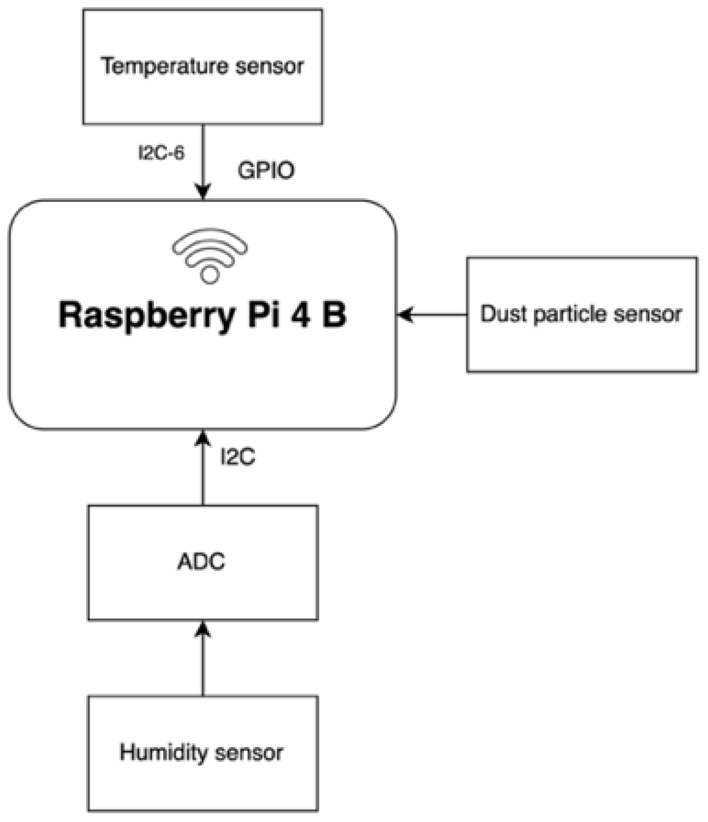
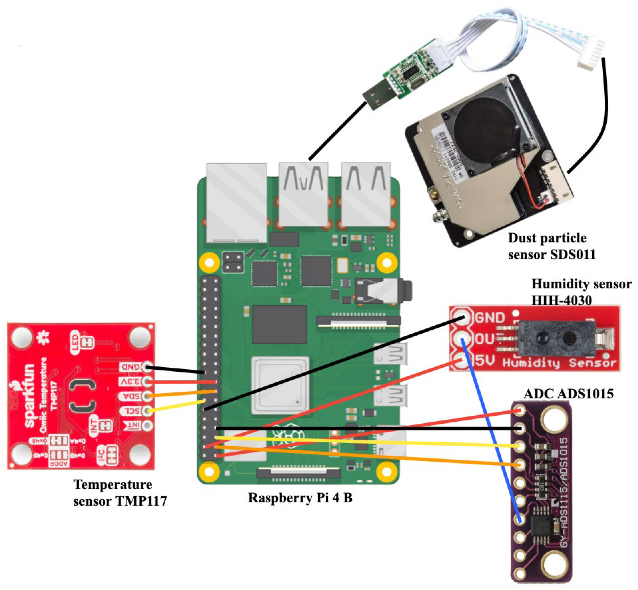
3.1. Hardware Part

Hardware represents the physical portion of a computer model, as opposed to software, which deals with the logical part.

Figure 2 presents the structure of the device. The processing unit with a Wireless Local Area Network (WLAN) module reads data from the connected sensors. The data are sent via HTTP to the cloud at configurable intervals (currently 1 min). The device has 3 sensors connected and is currently in use for temperature, humidity, and dust particles. The system could be easily extended with gas or other sensors.

3.1.1. Raspberry Pi 4 B

The Raspberry Pi 4 Model B offers enhanced multimedia capabilities, computing speed, memory, and networking with a 64-bit quad-core processor, dual displays, and PoE capability [28].

3.1.2. Temperature Sensor TMP117

TMP117 is a precise digital temperature sensor [29]. The temperature sensor uses digital data and Raspberry Pi’s GPIO pins for easy connection. To use the I2C communication protocol, SDA and SCL pins must be connected to microcontroller pins, requiring I2C-6 channel creation.

3.1.3. Humidity Sensor HIH-4030

The project utilized a SparkFun breakout board for Honeywell’s HIH-4030 humidity sensor, measuring relative humidity and providing an analog output voltage for easy data processing [30]. The analog sensor requires a converter from analog data into digital values for humidity calculation, influenced by ambient temperature using Formula (1).

$$True RH={\displaystyle \frac{SensorRH}{1.0546-0.00216T}} , T in °C,$$

(1)

3.1.4. Analog–Digital Converter ADS1015

ADS1015 is a precision 12-bit ADC with an on-board reference, oscillator, and I2C-compatible serial interface [31]. The converter uses the I2C communication protocol, so I connected it directly to the pins specific to this communication.

3.1.5. Dust Particle Sensor SDS011

SDS011 is an air quality sensor that measures dust particles and smoke concentrations, ensuring stability and security [32]. The sensor sends binary data on a serial port, which can be read directly using a UART controller or a USB serial connector. The SDS011 is connected to a Raspberry Pi using a serial adapter.

Figure 3 shows the electrical connection of each sensor to the microcontroller. To make this possible, mother–mother threads are used to connect the sensor to the development board. One end of the wire is connected to one of the sensor pins, and the other end to the corresponding pin of the plate.

Figure 4 depicts the electrical diagram and shows how each sensor is connected to the microcontroller. In the provided diagram, the color coding for the connections is as follows: red wires are used for power connections (3.3 V and 5 V), black wires are used for ground connections, yellow wires represent SDA (I2C data), orange wires are for SCL (I2C Clock), blue wires are used for the analog output from the HIH 4030 to A0 on the ADS 1015, and green wires are for the connections to the SDS011.

The flow diagram below indicates the process of data gathering and transmission via an IoT device and describes a data-gathering system based on a Raspberry Pi. The method begins with turning on the Raspberry Pi, and then running an application that activates the sensors to collect data. The system then looks for a Wi-Fi connection; if one is not available, the program terminates. If Wi-Fi is enabled, the system connects to a cloud database, and transfers and stores the collected data. After storing, the system waits for one minute before starting the next data collection cycle. The process comes to an end when the application is stopped (Figure 5).

3.2. Software Part

This component oversees gathering data, delivering it to a database, and predicting it. Software is a collection of instructions, data, or programs used to run machines and complete certain tasks.

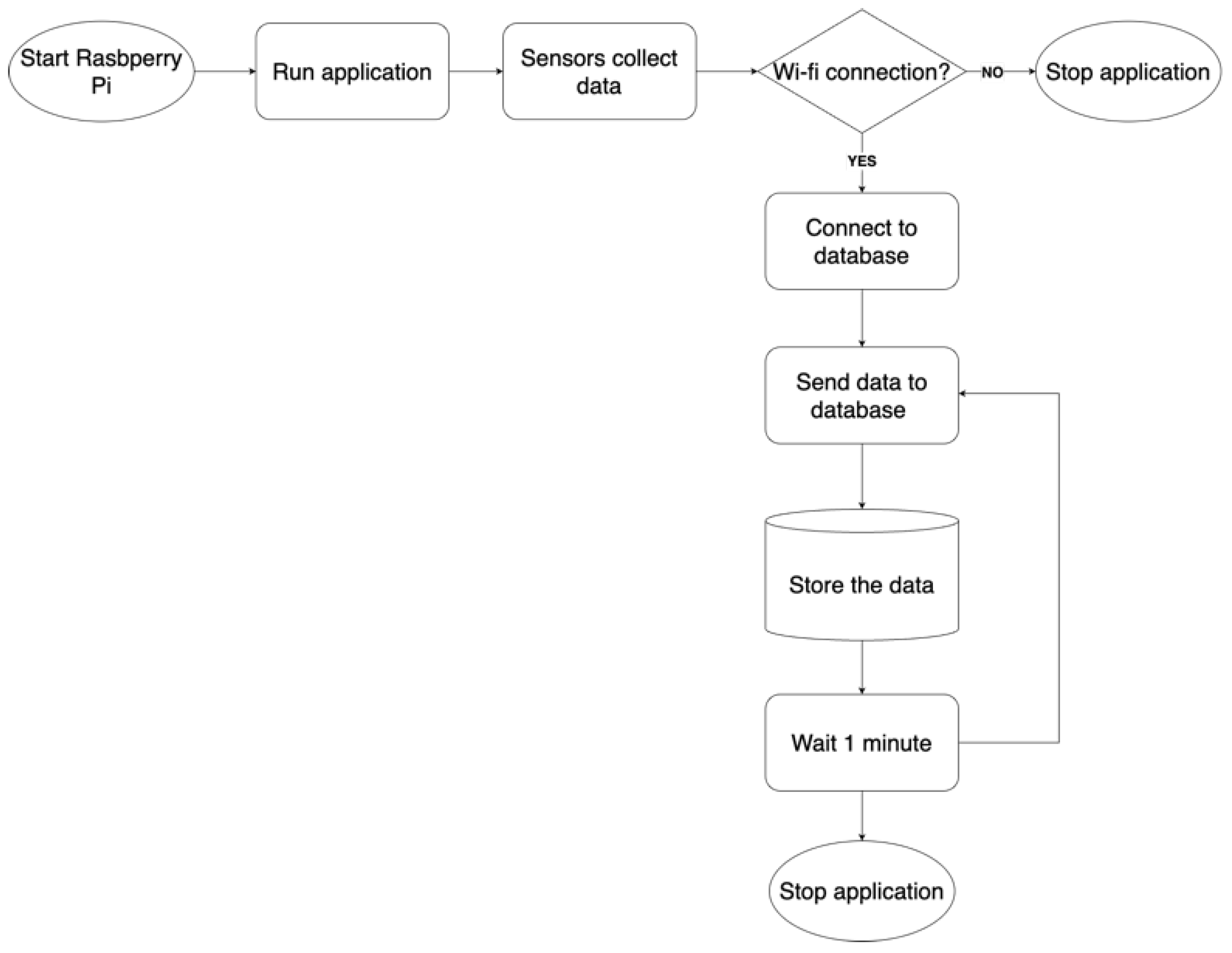
3.2.1. Acquisition of Data by Sensors

The Raspberry Pi microcontroller works by running an application developed using the Python 3.9 programming language.

Using the values from collected PM10 and PM2.5, AQI is calculated as in (2). To make this possible is required the installation of the python library python-aqi [33]. This library converts the AQI value to the pollutant concentration (µg/m³ or ppm) using the United States Environmental Protection Agency (EPA) algorithm [34,35] (Table 1).

$$I={\displaystyle \frac{I_{high}-I_{low}}{{BP}_{high}-{BP}_{low}}}·\left(C-{BP}_{low}\right)+I_{low},$$

(2)

where

I = the (Air Quality) index

C = the pollutant concentration

BP_low = the concentration breakpoint that is ≤C

BP_high = the concentration breakpoint that is ≥C

I_low = the index breakpoint corresponding to C_low

I_high = the index breakpoint corresponding to C_high

Table 1. AQI ranges.

Daily AQI Color	Levels of Concern	Values of Index	Description of Air Quality
Green			Air quality is satisfactory,
	Good	0 to 50	and air pollution poses
			little or no risk.
Yellow			Air quality is acceptable. However, there may be a risk for some people,
	Moderate	51 to 100	particularly those who are usually
			sensitive to air pollution.
Orange			Members of sensitive groups
	Unhealthy for Sensitive Groups	101 to 150	may experience health effects. The public is less likely to be affected.
Red			Some members of the general
	Unhealthy	151 to 200	public may experience health effects: members of sensitive groups may experience more serious health effects.
Purple			Health alert: The risk to health
	Very Unhealthy	201 to 300	effects is increased for everyone.
Maroon			Health warning of emergency
	Hazardous	301 and higher	conditions: everyone is more
			likely to be affected.

Table 1. AQI ranges.

Daily AQI Color	Levels of Concern	Values of Index	Description of Air Quality
Green			Air quality is satisfactory,
	Good	0 to 50	and air pollution poses
			little or no risk.
Yellow			Air quality is acceptable. However, there may be a risk for some people,
	Moderate	51 to 100	particularly those who are usually
			sensitive to air pollution.
Orange			Members of sensitive groups
	Unhealthy for Sensitive Groups	101 to 150	may experience health effects. The public is less likely to be affected.
Red			Some members of the general
	Unhealthy	151 to 200	public may experience health effects: members of sensitive groups may experience more serious health effects.
Purple			Health alert: The risk to health
	Very Unhealthy	201 to 300	effects is increased for everyone.
Maroon			Health warning of emergency
	Hazardous	301 and higher	conditions: everyone is more
			likely to be affected.

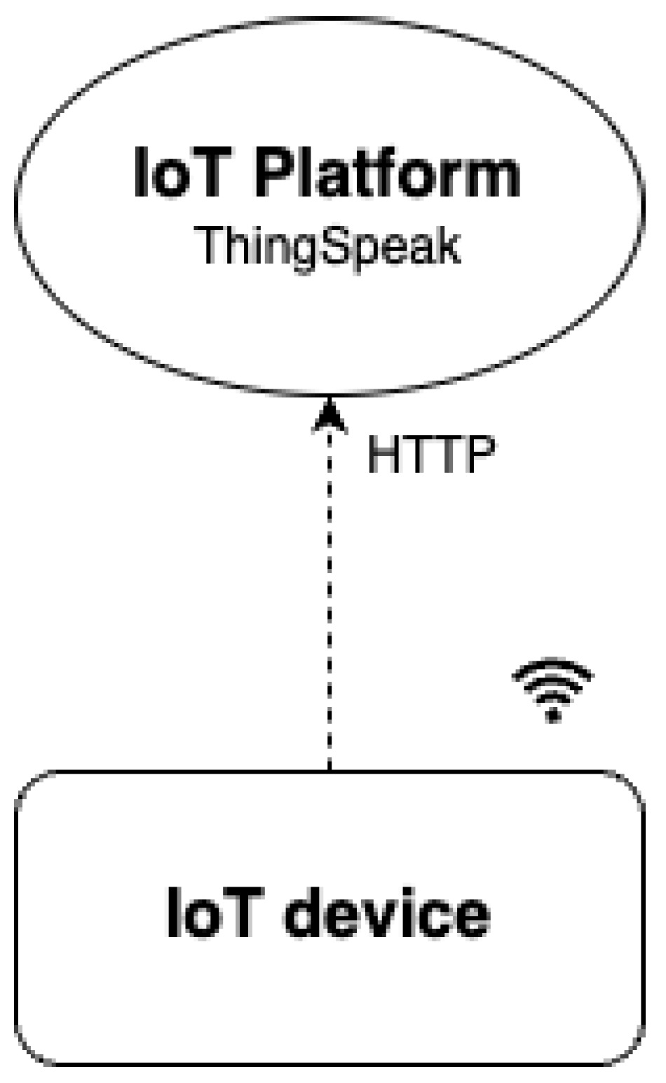
3.2.2. ThingSpeak Cloud Computing Platform

The collected data are sent to ThingSpeak, which is an ‘Application Programming Interface’ (API) and web service for the ‘Internet of Things’ (IoT) [36]. ThingSpeak serves as a valuable tool for displaying and analyzing the environmental data collected through the IoT-based monitoring system implemented in the study. A new channel is created on ThingSpeak and data is sent to it using an HTTP GET request. The URL was constructed with the Write API Key and the appropriate field values, enabling the transmission of data to the ThingSpeak platform for visualization and analysis.

The communication between the collecting stations and the central node is wireless. At 1 min intervals, samples of data are collected and sent to the device. In order to connect and send data to the ThingSpeak platform, the device is connected to a Wireless Local Area Network (WLAN) and Hyper-Text Transfer Protocol (HTTP) is used, as can be seen in Figure 6.

ThingSpeak offers 4 channels for free, where each channel can contain a maximum of 10 fields. As the implemented IoT system collects 6 factors, only 6 fields are required. After creating the channel, it is accessible through an API key. Having only 1 collecting device, this channel is enough for this IoT system. Uploading data to ThingSpeak is made with HTTP requests. A GET method is called to the ThingSpeak platform’s URL with the parameters—the API key and the values for the 6 fields (e.g., url):

$$\begin{array}{cc}URL& =f^{\prime }https://api.thingspeak.com/update?api\_key=““\&field1\hfill \\ & \hspace{1em}\hspace{1em}\hspace{1em}\hspace{1em}=\{temp\_db\}\&field2=\{hum\_db\}\&field3=\{pm\_ten\_db\}\&field4\\ & \hspace{1em}\hspace{1em}\hspace{1em}\hspace{1em}=\{pm\_twofive\_db\}\&field5=\{aqi\_ten\_db\}field6\\ & \hspace{1em}\hspace{1em}\hspace{1em}\hspace{1em}=\{aqi\_twofive\_db{\}}^{\prime }\end{array}$$

The method of uploading data from the device was chosen due to the fact that connecting the collecting station to the internet would increase the power consumption of the microcontroller. In this way, the running time of the device increases.

The data are precisely read by the sensors, which include the temperature sensor, humidity sensor, dust sensor, and index quality, as illustrated in Figure 7, and thus, no human intervention is required in the sensing process. The IoT device is responsible for collecting the environmental parameters, for processing the raw data and calculating the air quality index based on the particle matter data, and for transmitting the data to the cloud database using Wi-Fi.

The second component represents the cloud database, and it oversees storing the transmitted data securely for real-time and historical analysis. It also provides functionality to export the stored data as a CSV file for further analysis.

The last part is represented by the data analysis and prediction model. Firstly, the dataset must be imported for analysis. Then, the prediction model would be created using TensorFlow-based analysis. In the end, the resulting data will be displayed and visualized for easy interpretation by the user.

3.2.3. Making Predictions

The proposed system imports the air quality dataset into Google Collab, saving it in CSV format for easy computer analysis. These data are easily analyzed using the TensorFlow (version 2.17.0) package included with the Google Collab program. TensorFlow [37] is an open-source machine learning library developed by Google that offers two modes of execution: the eager mode and graph mode.

The dataset includes 6 critical parameters that aid in air quality prediction. Initially, the dataset is preprocessed using appropriate approaches to remove inconsistent and missing valued data, and the necessary features from the dataset are chosen to improve the outcomes. The dataset is then divided into two parts: training and testing to evaluate the model’s performance.

Regression analysis [38] is a type of predictive modeling technique that examines the relationship between a dependent and an independent variable. This technique is used for forecasting or predicting, time series modeling, and determining the causal relationship between variables.

• Air quality dataset collection

The project uses an air quality dataset from the ThingSpeak cloud, available in CSV format. The data, spanning 5 days from 17 to 21 May 2024, and taken from an office with two people, offers information on the average minute reactions of air components. The dataset has 5869 rows and 8 columns.

2.

Data preprocessing

This is a data mining method that converts raw data into a comprehensible format by cleansing it, filling in missing values, smoothing noisy data, resolving inconsistencies, and converting decimal values to suitable floats.

The errors or inconsistencies in the data are identified and corrected. This involves removing duplicates, handling outliers, and correcting data entry errors. The missing values are handled. The data are normalized or standardized by converting them to a consistent scale, which is often necessary for algorithms that require normalized input data. Decimal values are converted to suitable floats to maintain precision and ensure consistent analysis.

In detail, the following preprocessing steps have been performed:

• Handling Missing Values: The method dropna(inplace = True) addresses missing values by removing the rows with any missing data. This ensures that the dataset used for training and testing does not contain null or missing entries.
• Outlier Detection and Removal using IQR: Outliers are detected using the Interquartile Range (IQR) method. The IQR is calculated by subtracting the first quartile (Q1) from the third quartile (Q3). Outliers are defined as values that lie below Q1−1.5IQR or above Q3 + 1.5IQR. These rows are removed from the dataset.
• Data Transformation: The PowerTransformer with the yeo–johnson method [39] is used to transform the selected numeric columns (temperature, humidity, pm10, and pm25). The Yeo–Johnson transformation is suitable for data that include both positive and negative values. It adjusts the distribution to be more Gaussian-like without losing information. By making the data more Gaussian-like, it can often improve the performance and stability of the machine learning models.
• Converting Data Types to Float: To ensure consistency in the data format, the numeric columns are converted to float. This is crucial for accurate computations, especially in machine learning models, which often require numeric input data in the float format.
• Normalization or Standardization: The code uses the StandardScaler method to standardize the feature values. This scales the data so that it has a mean of 0 and a standard deviation of 1, which helps certain machine learning models perform better, especially those that are sensitive to the scale of input data.

3.

Splitting training and test dataset

Separating datasets into training and testing sets is a crucial step in evaluating data mining methods. Most data are used for training, while a smaller amount is used for testing. Create a model using training data and test it against the test set to minimize data discrepancies and improve model properties.

The data are split as follows: 80% was used to train the model and 20% was used for testing it. By training the model on one subset and testing it on another, it can be assessed how well the model generalizes to new data, helping to identify and minimize overfitting or underfitting.

4.

Feature selection

Machine learning models’ performance is heavily influenced by the data features used to train them. Irrelevant or partially relevant features may have a negative impact on the model performance. In this project, attributes such as ‘temperature’, ‘humidity’, ‘pm10′, and ‘pm25′ were chosen for better results. The relevance of a feature is measured as the entire reduction in criteria caused by that characteristic.

The feature importance is measured using various techniques, such as the following:

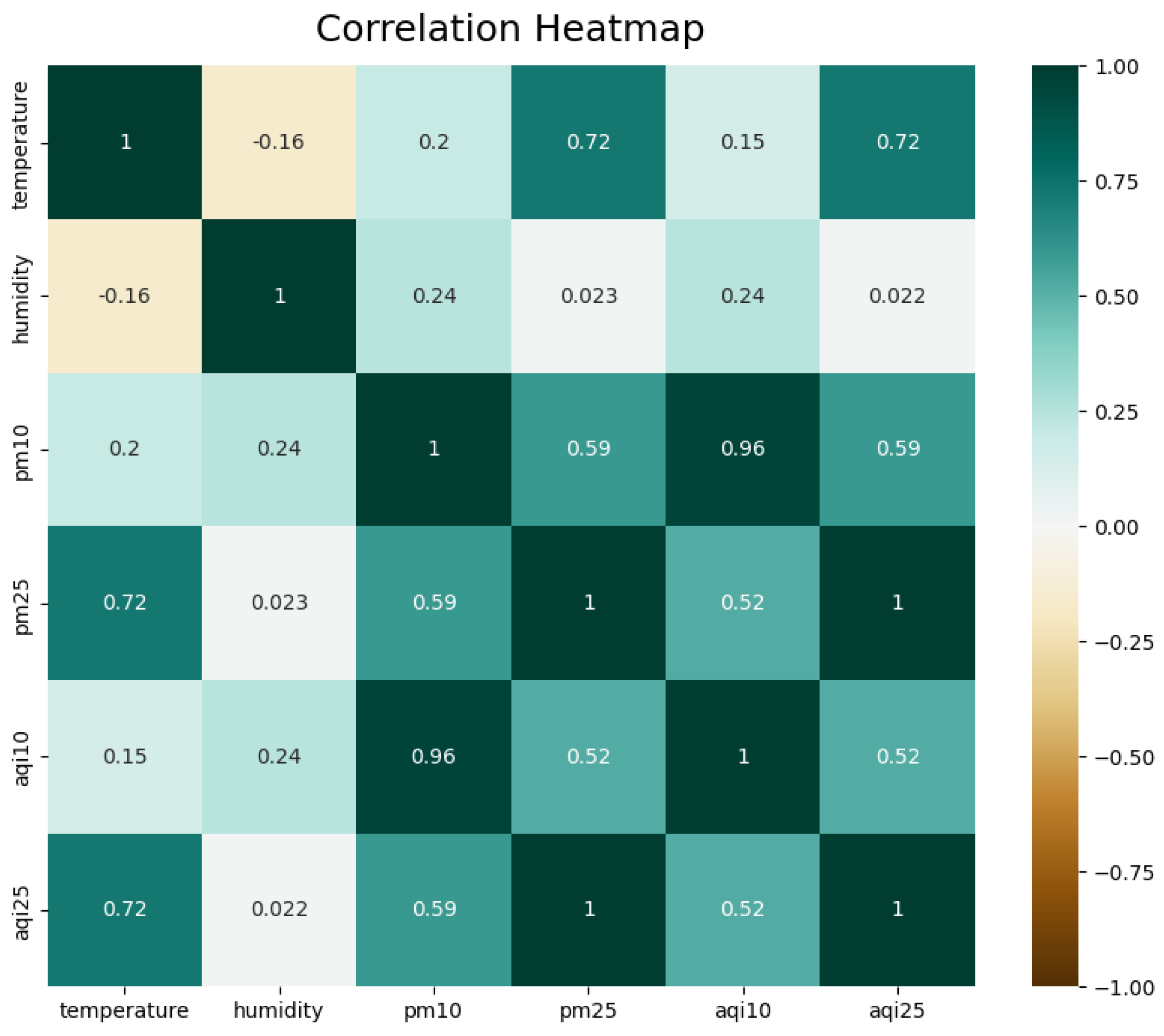
• Correlation Analysis: Evaluating the correlation between each feature and the target variable.
• Feature Importance Scores: Using algorithms like random forests to rank feature importance.

5.

Regression analysis

The processed datasets are used to generate a function that plots training and validation data for a sequential neural network with backpropagation learning. This model is designed for regression tasks, where the goal is to predict a continuous numerical value.

Linear regression is a widely used predictive analysis method that assesses the effectiveness of a group of predictor variables in predicting an outcome and identifies the most significant predictor variables. It is a statistical technique utilized to analyze the correlation between a dependent variable (y—which is the target prediction) and one or more independent variables (x) [40].

Consider the model function (3) which describes a line with slope β and y-intercept α.

$$y=\alpha +\beta x,$$

(3)

The scientific literature reveals the following benefits of using linear regression:

• Simplicity and Interpretability: Linear regression is a computationally efficient, simple, and easy-to-understand technique. The correlation between the variables is easily understood because the coefficients show the precise influence of each predictor.
• Low Variance: Compared to more complex models, linear regression is less prone to overfitting because it is based on a single model.
• Helpful for Small Datasets: It works effectively with smaller datasets with a linear relationship.

There are also disadvantages of linear regression:

• Assumption of Linearity: Linear regression assumes a linear relationship between the independent and dependent variables, which limits its effectiveness in capturing complex patterns.
• Sensitivity to Outliers: Linear regression is sensitive to outliers, which can distort the model and affect its prediction accuracy.
• Limited in Handling Multicollinearity: Multicollinearity among predictor variables can impact the stability of the model coefficients.

Backpropagation is a fundamental technique for training neural networks involving the backward propagation of mistakes. It involves computing the difference between the expected output and the actual target value and adjusting the weights based on this gradient. This technique helps the model learn from past failures and improve its predictions over time, thereby enhancing performance.

Random forest regression is a machine learning technique for predicting continuous outcomes by aggregating the predictions of numerous decision trees. It operates by building a ‘forest’ of decision trees during training, with each tree employing a random part of the training data and a random subset of the characteristics [41]. In random forest regression, the final prediction is obtained by averaging the predictions of all the individual trees in the forest, resulting in a more accurate and stable forecast than a single decision tree model. This strategy reduces the variance of regression predictors using bagging while keeping the bias largely constant.

Random forest (RF) regression overcomes some shortcomings of linear regressions. Thus, the main advantages of RF are as follows:

• Robustness to Outliers and Noise: RF models are resilient to outliers and noise due to their ensemble approach, which averages out extreme predictions from individual trees.
• Ability to Capture Non-Linear Relationships: Unlike linear regression, random forests can model complex, non-linear relationships between the predictor and response variables.
• Feature Importance: RF can rank the importance of variables, providing insights into which predictors have the most influence on the outcome.

However, there are some disadvantages specific to random forest regression:

• Complexity and Interpretability: Unlike linear regression, RF models are complex and less interpretable, making it difficult to understand how individual predictions are made.
• Higher Computational Cost: RF requires more computational resources and time, especially with large datasets and many trees.
• Tendency to overfit: Although reduced by bagging, random forests can still overfit, particularly when too many trees are used or if not properly tuned.

Judging from practical reasons, linear regression is suitable for simple, small-scale problems where interpretability and low variance are crucial. Instead, random forest regression is better suited for complex tasks with larger datasets, high dimensionality, and where capturing non-linear interactions among variables is essential.

In this work, we preferred both linear regression due to its simplicity and small dataset produced by the IoT system, but also random forest regression for its benefit of robustness to outliers and noise and the ability to capture non-linear relationships between the predictor and response variables.

6.

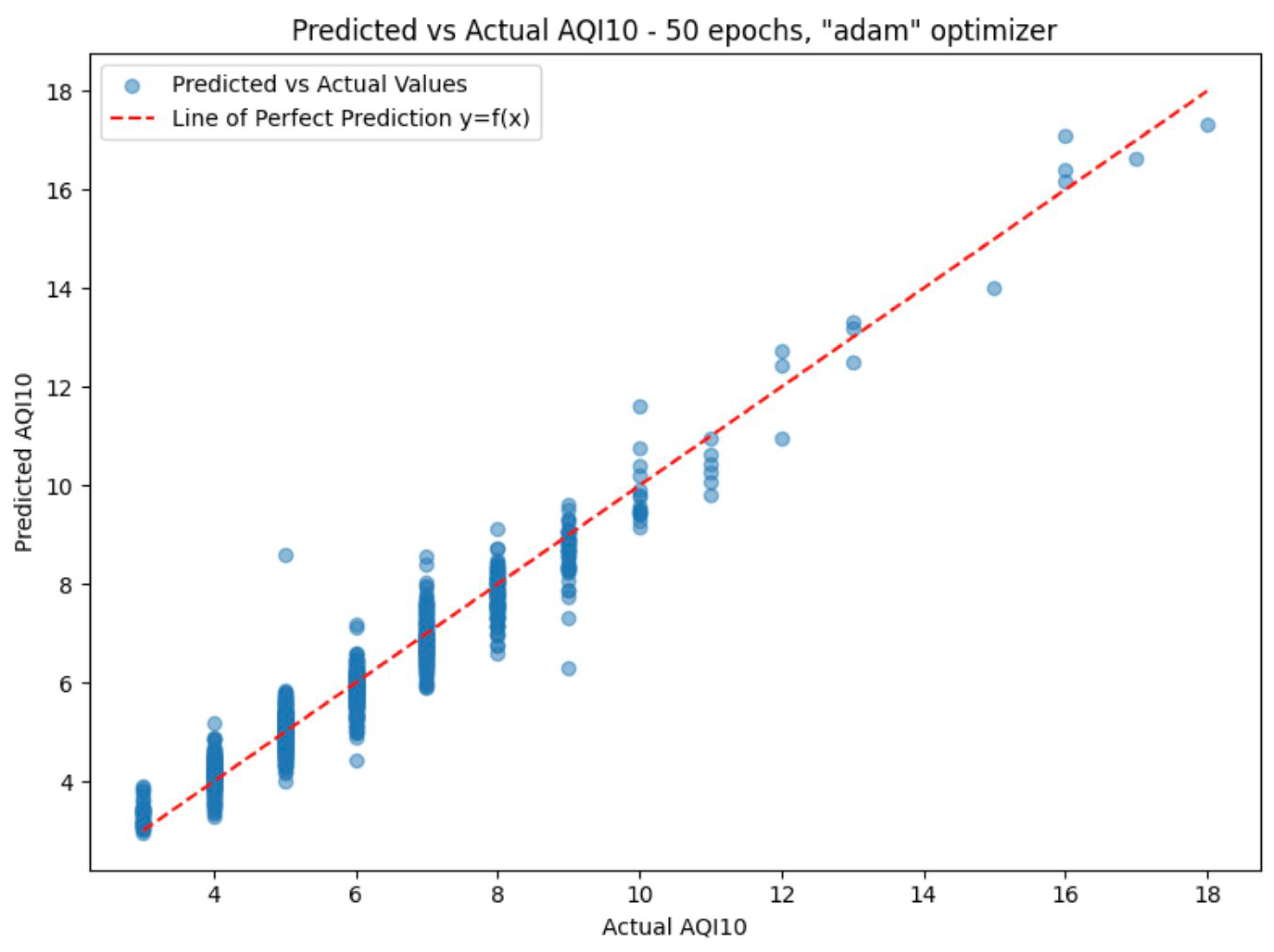
Air quality prediction metrics

The Mean Absolute Error (MAE) is a statistical measure used to evaluate the performance of a regression model, calculating the average difference (4) between the model’s predicted and actual data values. It is also known as the L1 loss function and is calculated by dividing the number of observations by the predicted value.

$$MAE={\displaystyle \frac{{\sum }_{i=1}^n\left|y_i-{\widehat{y}}_i\right|}{n}},$$

(4)

where

n is the number of observations in the dataset.

y_i is the true value.

ŷ_i is the predicted value.

R-squared, also known as the coefficient of determination, is the proportion of variance in the dependent variable that can be predicted from the independent variables in a regression model (5). It has a value between 0 and 1, with 1 indicating that the model accounts for all the variability in the data and 0 indicating that none of it does [42].

$$R^2=1-{\displaystyle \frac{{SS}_{RES}}{{SS}_{TOT}}}=1-{\displaystyle \frac{{\sum }_i{\left(y_i-{\widehat{y}}_i\right)}^2}{{\sum }_i{\left(y_i-\overline{y}\right)}^2}},$$

(5)

where

${SS}_{RES}$ is the sum of the squares of the residual errors (the difference between the observed and predicted values).

${SS}_{TOT}$ is the total sum of squares (the difference between the observed values and their mean, squared).

Mean squared error (MSE) is a statistical measure that quantifies the average squared difference between the observed and predicted values (6). After calculating the squared difference for each data point, the average of those squared differences is calculated. MSE is more prone to outliers than MAE since it allocates higher weights to errors [43].

$$MSE={\displaystyle \frac{\sum {\left(y_i-{\widehat{y}}_i\right)}^2}{n}},$$

(6)

The square root of MSE is referred to as the root mean squared error (RMSE). This measure is frequently used since it is simple to read and has the same unit as the dependent variable. It gives an indicator of the average error magnitude [44].

The root mean squared error (RMSE) is one of two primary performance measures for a regression model. It calculates the average difference between the values predicted by a model and the actual values. It estimates the model’s ability to predict the target value (7).

$$RMSE=\sqrt{MSE}=\sqrt{{\displaystyle \frac{\sum {\left(y_i-{\widehat{y}}_i\right)}^2}{n}}},$$

(7)

The model performs better when the root mean squared error decreases. A perfect model (a hypothetic model that consistently predicts the precise expected value) would have a root mean squared error of zero.

In statistics, the Mean Absolute Percentage Error (MAPE), sometimes referred to as mean absolute percentage deviation (MAPD), is a metric of forecasting method prediction accuracy. MAPE is the average of Absolute Percentage Errors (APEs). Let A_t and F_t denote the actual and forecast values at data point t, respectively [45]. It typically expresses accuracy as a ratio specified by the following Formula (8), where N is the number of data points:

$$MAPE={\displaystyle \frac{1}{N}}\sum _{t=1}^N\left|{\displaystyle \frac{A_t-F_t}{A_t}}\right|\times 100,$$

(8)

However, MAPE has one big drawback: it generates infinite or undefined results when the actual values are 0 or close to zero, which is typical in particular domains. If the real values are very tiny (often less than one), MAPE produces extraordinarily large percentage mistakes (outliers), whereas zero actual values produce endless MAPEs.

The Root Mean Squared Logarithmic Error (RMSLE) is determined by applying the log function to the actual and predicted values and then subtracting them. RMSLE is resistant to outliers when both minor and large errors are considered [46].

$$RMSLE=\sqrt{{\displaystyle \frac{1}{N}}\sum _{i=0}^N{(\log \left(y_i+1\right)-\log \left({\widehat{y}}_i+1\right))}^2},$$

(9)

Symmetric Mean Absolute Percentage Error (SMAPE) is a modified version of MAPE that accounts for symmetry, providing a balanced measure of prediction error relative to both the actual and predicted values [47]. SMAPE is a modified MAPE where the divisor is half the sum of the actual and forecast values, addressing MAPE’s issue with outliers by providing a symmetric measure of forecast accuracy. It is usually defined as follows (10):

$$SMAPE={\displaystyle \frac{100}{N}}\sum _{t=1}^N{\displaystyle \frac{\left|F_t-A_t\right|}{\frac{\left|A_t\right|+\left|F_t\right|}{2}}},$$

(10)

The absolute difference between $A_t$ and $F_t$ is calculated by dividing the sum of the absolute values of the actual and predicted values by half. The result of this calculation is added for each fitted point t and then divided by the number of fitted points N.

Mean Directional Accuracy (MDA) measures how often the predicted direction of change matches the actual direction of change. It is useful for time series and directional forecasts. It compares the forecast direction (upward or downward) to the actual realized direction. It is defined by the following Formula (11), where $y_i$ is the actual value at time i and ${\widehat{y}}_i$ is the forecast value at time i. Variable N represents the number of forecasting points and I[⋅] is the indicator function that equals 1 if the condition inside is true and 0 otherwise.

$$MDA={\displaystyle \frac{1}{N}}\sum _{i=2}^N\mathsf{{\rm I}} [\left(y_i-y_{i-1}\right)·\left({\widehat{y}}_i-{\widehat{y}}_{i-1}\right)>0]$$

(11)

The Median Absolute Error (MedAE) is a robust statistical measure used to evaluate the accuracy of predictions, particularly in the presence of outliers. It is defined as the median of the absolute differences between the predicted and actual values, making it less sensitive to extreme values compared to other metrics like Mean Absolute Error (MAE) or Root Mean Square Error (RMSE).

The loss is calculated by taking the median of all the absolute differences between the target and the prediction, by following Formula (12):

$$MedAE=median \left|y_i-{\widehat{y}}_i\right|,$$

(12)

In the source code, we easily changed the methods depending on the needs (e.g., from ‘tf.keras.metrics.MeanSquaredError’ to ‘tf.keras.metrics.MeanAbsolutePercentageError’) when compiling the model.

4. Results

The graphs presented below were generated in the ThingSpeak platform based on the data collected by the implemented IoT device. Figure 8 and Figure 9 represent the charts that contain all the entries of AQI 10 and AQI 2.5, respectively, in the database.

The simple method of graphing and calculating using a machine learning methodology is discussed below.

Figure 10 depicts a heat map of the air quality dataset’s properties in a graphical format. The color scale runs from −1 to 1, with dark green indicating stronger positive correlations (closer to 1), brown indicating stronger negative correlations (closer to −1), and white or light green expressing no correlation (closer to zero).

Based on the provided heatmap, AQI 2.5 shows a strong positive correlation with temperature and PM2.5, indicating that as these parameters increase, AQI 2.5 also increases significantly. Additionally, AQI 2.5 has moderate positive correlations with PM10 and AQI10, suggesting a moderate relationship with these parameters. However, AQI 2.5 does not exhibit strong correlations with temperature or humidity, as indicated by their lower correlation values. On the other hand, AQI 10 demonstrates moderate positive correlations with both PM10 and PM2.5, but it does not show strong correlations with temperature or humidity. This analysis highlights that while AQI 2.5 and AQI 10 are influenced by particulate matter levels, they are not significantly affected by temperature and humidity.

The model is trained using both types of regression analysis: linear regression and random forest regression. For linear regression are used different numbers of epochs (50, 100, 500, and 1000), and for random forest, two values for the number of decision trees (100 and 1000). The following figures represent the accuracy of the predictions by 50 epochs.

The following 5 figures (Figure 11, Figure 12, Figure 13, Figure 14, Figure 15 and Figure 16) compare the actual AQI 10 or AQI 2.5 with the predicted one. Each scatter plot used displays the actual values of AQI along the X-axis, and displays the predicted values along the Y-axis. Each point represents individual data entries, and the dashed red line indicates the ideal relationship where the predicted values exactly match the actual measurements. Correlating the results from Figure 11, Figure 12, Figure 13, Figure 14, Figure 15 and Figure 16 with the previous charts (Figure 8 and Figure 9—Graph generated in ThingSpeak web application for AQI), it is easier to understand why for a single value on the X-axis (taken at different times in the measurement interval) there are more (predicted) values on the Y-axis. To some extent, this is also the purpose of machine learning algorithms to reduce the prediction error over multiple iterations.

The results in Figure 11 are obtained after the dataset was trained using the ‘adam’ optimizer for the prediction model while Figure 12 contains the results using the ‘RMSprop’ optimizer. It can be observed that this model is more accurate than the other one.

The following diagrams compare the actual with the predicted value of AQI 2.5. Most of the data points which can be seen in the Figure 13 cluster more closely around the red dashed line than the ones from the diagram represented in Figure 14, suggesting that the first model’s predictions are more accurate than the other one.

The values obtained indicate that our model prediction is performing well and according to Figure 11 and Figure 13, our data fits into the ‘good’ range from the AQI categories, which can be seen in the Table 1 [35]. However, the low values of AQI can be due to the rather high temperatures (above 22 degrees Celsius) from the time of data collection—May 2024, because it is known that PM ratios decrease with increasing temperature [2]. On the other hand, the particular context of the analyzed environment with less household activities like cooking on stoves and indoor smoking positively affected the less indoor particulate emissions.

The Figure 15 and Figure 16 represent the accuracy of the predictions by 1000 epochs using random forest regression.

Table 2. AQI measurements resulted after evaluating the model with MAE, MSE, RMSE and R2.

Prediction Model	Epochs	AQI 10				AQI 2.5
		MAE	MSE	RMSE	R2	MAE	MSE	RMSE	R2
‘adam’ optimizer	50	0.3289	0.1968	0.4437	0.9383	0.3205	0.1557	0.3946	0.9953
	100	0.3276	0.1972	0.4440	0.9382	0.3211	0.1573	0.3966	0.9952
	500	0.3246	0.2032	0.4508	0.9363	0.3247	0.1622	0.4028	0.9951
	1000	0.3174	0.2102	0.4585	0.9341	0.3145	0.1494	0.3865	0.9955
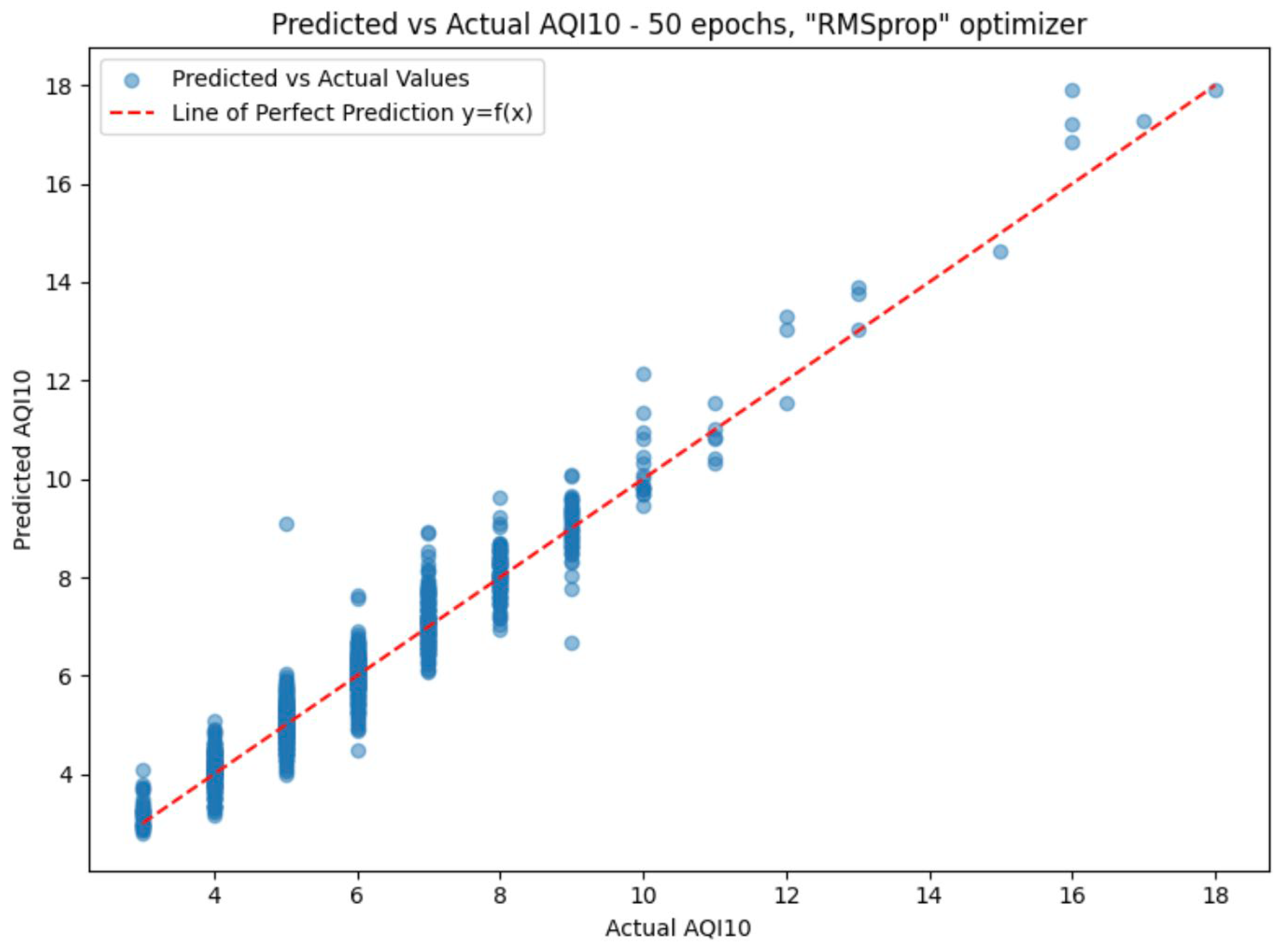
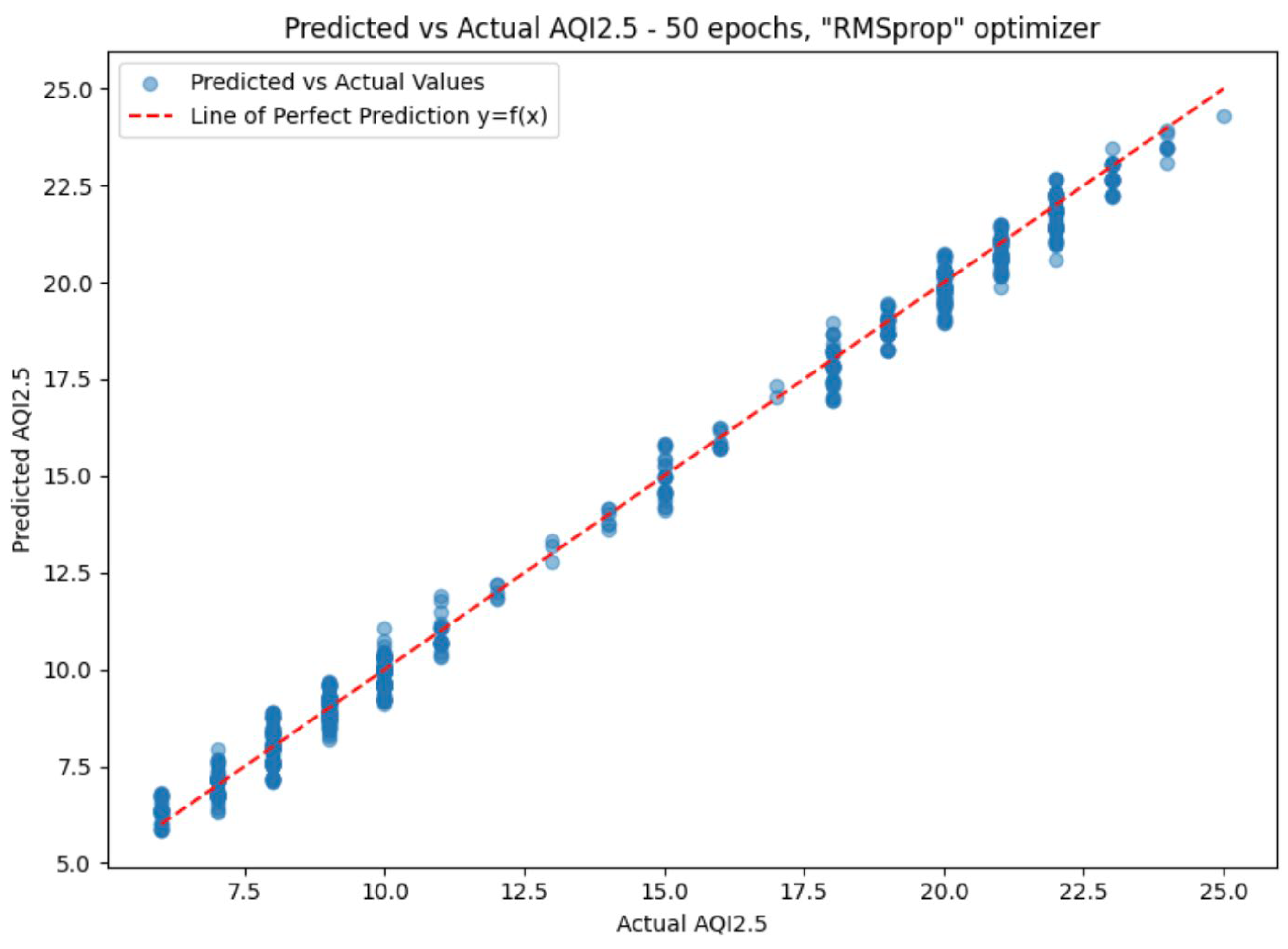
‘RMSprop’ optimizer	50	0.3550	0.2202	0.4693	0.9309	0.3283	0.1678	0.4096	0.9949
	100	0.3142	0.1901	0.4360	0.9404	0.3432	0.1795	0.4237	0.9946
	500	0.3145	0.1995	0.4467	0.9374	0.3222	0.1581	0.3976	0.9952
	1000	0.3088	0.2018	0.4492	0.9367	0.3361	0.1690	0.4111	0.9949
	n_estimator
Random Forest	100	0.2785	0.2095	0.4577	0.9343	0.2483	0.1516	0.3894	0.9954
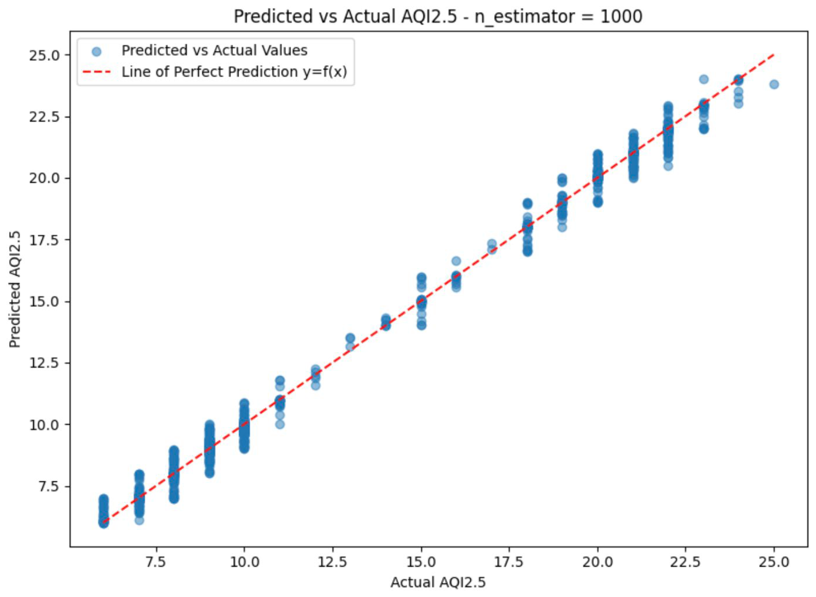
	1000	0.2778	0.2086	0.4568	0.9346	0.2482	0.1503	0.3877	0.9955

reflect the results generated by the Mean Absolute Error, Mean Squared Error, Root Mean Squared Error, and R-squared metrics.

The ‘adam’ optimizer’s performance improves with increasing epochs, with a slight decrease in the Mean Absolute Error (MAE) for AQI 10 and a similar trend for AQI 2.5. The root mean squared error (RMSE) also decreases with more epochs, suggesting better predictions. The R-squared values are consistently high for both AQI 10 and AQI 2.5, indicating that the model explains a significant portion of the data’s variance. This suggests that the ‘adam’ optimizer is effective in predicting data.

The ‘RMSprop’ optimizer significantly improves the MAE for AQI 10 from 0.35508 to 0.30883 at 1000 epochs, while the MAE for AQI 2.5 initially increases but decreases to 0.33618 at 1000 epochs. The RMSE for both AQI 10 and AQI 2.5 follows a similar trend, improving with more epochs. The R2 values remain high, indicating the optimizer effectively explains data variance, though slightly lower than the ‘adam’ optimizer.

The random forest model with 100 estimators has a lower MAE for AQI 10 and AQI 2.5 compared to the neural network models using the ‘adam’ and ‘RMSprop’ optimizers. Increasing the number of estimators slightly reduces the MAE, indicating a marginal improvement. The RMSE values are comparable to the neural network models, and the R2 values are high, indicating a strong fit to the data.

Table 3. AQI measurements resulted after evaluating the model with MAPE, RMSLE, SMAPE, MDA and MedAE.

Prediction Model	Epochs	AQI 10					AQI 2.5
		MAPE	RMSLE	SMAPE	MDA	MedAE	MAPE	RMSLE	SMAPE	MDA	MedAE
‘adam’ optimizer	50	5.8233	0.0641	2.8391	0.8181	0.2574	2.9556	0.0350	1.4827	0.8973	0.3009
	100	5.7407	0.0651	2.8698	0.8172	0.2519	3.0036	0.0349	1.4933	0.8973	0.2807
	500	5.6104	0.0639	2.7885	0.8163	0.2472	2.8540	0.0335	1.4272	0.9019	0.2716
	1000	5.5584	0.0643	2.7145	0.8154	0.2268	2.8293	0.0333	1.4046	0.9001	0.2645
‘RMSprop’ optimizer	50	5.7068	0.0644	2.8106	0.8154	0.2501	3.0410	0.0360	1.5331	0.8992	0.3048
	100	5.9537	0.0656	2.8735	0.8145	0.2581	3.0137	0.0357	1.4772	0.8973	0.2952
	500	5.5275	0.0633	2.7228	0.8127	0.2385	3.0861	0.0357	1.5194	0.9001	0.2990
	1000	5.6649	0.0665	2.7507	0.8108	0.2193	3.0040	0.0357	1.5155	0.9000	0.3023
	n_estimator
Random Forest	100	4.8627	0.0662	4.7675	0.8151	0.1300	2.3673	0.0351	2.3568	0.8997	0.1100
	1000	4.8703	0.0662	4.7767	0.8099	0.1340	2.3608	0.0348	2.3490	0.8971	0.1140

summarizes the findings generated by the Mean Absolute Percentage Error, Root Mean Squared Log Error, Symmetric Mean Absolute Percentage Error, Mean Directional Accuracy, and Median Absolute Error metrics.

For the ‘adam’ optimizer, as the epochs increase from 50 to 1000, there is a noticeable improvement in the accuracy metrics for both AQI PM10 and PM2.5. For instance, the MAPE for AQI PM10 decreases from 5.8233 at 50 epochs to 5.5584 at 1000 epochs, while the SMAPE drops from 2.8391 to 2.7145, indicating a reduction in error.

Similarly, for AQI PM2.5, the MAPE reduces from 2.9556 at 50 epochs to 2.8293 at 1000 epochs, and the MedAE decreases from 0.3009 to 0.2645, demonstrating enhanced prediction accuracy with more training.

In contrast, the ‘RMSprop’ optimizer exhibits fluctuating results across epochs; for example, the MAPE for AQI PM10 varies from 5.7068 to 5.6649, while the MDA slightly decreases from 0.8154 to 0.8108. AQI PM2.5 performance remains relatively stable, with the MDA around 0.9000 but some inconsistencies in other metrics like the SMAPE and MedAE.

The random forest model, evaluated with 100 and 1000 estimators, shows consistent performance, maintaining a lower MAPE of around 4.8627 for AQI PM10 and 2.3673 for AQI PM2.5 compared to the optimizers. However, the SMAPE values are higher, such as 4.7675 for AQI PM10, highlighting differences in how errors are distributed.

Overall, the ‘adam’ optimizer demonstrates gradual improvement with more epochs, the ‘RMSprop’ optimizer shows mixed stability, and random forest provides consistent but distinct error dynamics, especially in the MAPE and SMAPE comparisons.

5. Discussions

One limitation of our study is that the IoT system has been tested indoors. Even if from a physical point of view the IoT system can be relatively easily adapted for outdoor environments, in the following is provided a more comprehensive analysis from a holistic view (physical, economical, authorization and legislation, etc.).

Outdoor air quality monitoring comes with some challenges besides adding sensors. First of all, it is about powering the IoT systems, developed and placed on poles, to voltage sources (either for direct connection to the city network power grid or using solar batteries) but the latest will offer a different lifetime from one area to another, from a season to another, and variability including in the collection of data from the sensors. Another challenge consists of transmitting data to the cloud and ensuring the level of connectivity of the IoT system (wired networks, Wi-Fi, RFID, GSM, etc.). These constraints, besides the number of systems implemented and arranged on poles approximately 200 m apart, will have an economic impact. Another impediment in outdoor implementation is the agreement of local or county authorities to place IoT systems in the city for monitoring as well as ensuring their maintenance in the case of malfunctions. The system implemented in this phase and support for the scientific paper is only a prototype with the aim of generating data that can then be used in the application of artificial intelligence algorithms for prediction. The IoT system was tested internally to avoid some of the previously mentioned challenges.

However, in 2017, one of the co-authors had such a development for outdoor air quality monitoring using a prototype connected to cars, GSM for data transmission using mobile phones, and GPS sensors to identify the geographic position with impact in the case of changes in weather conditions [4]. Sensors that must be added for outdoor monitoring are a gas sensor for measuring CO₂ and NOX (e.g., SainSmart MQ135 Sensor Air Quality Sensor and Hazardous Gas Detection Module) and barometric pressure (e.g., BMP085 Digital Barometric Pressure Measurement Sensor). For communication could be used either a combined GPS/GSM unit for location and communication or a Wi-Fi connectivity and GPS unit. Another limitation consists of the relatively small dataset and using machine learning algorithms with fixed parameters. For any kind of optimization problem, the hyperparameters can be tuned and varied in a design space exploration process. An automatic design space exploration process based on genetic algorithms or other evolutionary algorithms consumes a lot of execution time and was not the initial scope of this work. However, the idea will be investigated by the authors as a further development.

Despite these limitations, the current work has succeeded in presenting an integrated AIoT system in which the physical IoT system is functional and produces real data regarding air pollution which are then analyzed and used as input in machine learning algorithms (AI component of the system) for the implementation of prediction algorithms. The random forest model expresses the best performance exploiting the robustness to outliers and noise and the ability to capture non-linear relationships between the predictor and response variables.

6. Conclusions and Further Work

This study presents an integrated IoT system developed by the authors for evaluating the performance of different machine learning models in predicting air quality indices (AQI 10 and AQI 2.5) based on various features such as temperature, humidity, PM10, and PM2.5 concentrations.

Specifically, it compared the effectiveness of neural network models trained with the ‘adam’ and ‘RMSprop’ optimizers over different epochs with a random forest model with varying numbers of estimators. The key metrics used for evaluation included the Mean Absolute Error (MAE), mean squared error (MSE), root mean squared error (RMSE), and R-squared (R2).

Both the ‘adam’ and ‘RMSprop’ optimizers show improvements in the MAE and RMSE with increasing epochs. However, the random forest model outperforms the neural network models for both AQI 10 and AQI 2.5 in terms of the MAE. The random forest model with 100 or 1000 estimators provides the best performance.

Finally, monitoring indoor parameters using IoT devices is motivated by a desire to build healthier and more sustainable interior environments. Researchers intend to improve occupant well-being and productivity by addressing research issues such as sensor technology, data management, user experience, health implications, calibration and validation, integration, and interoperability.

In a longer perspective, our aim is to further develop the device by incorporating more diverse sensors (like gas detection, barometric pressure, etc.) to measure other pollutants (nitrogen dioxide, nitric oxide, carbon monoxide, carbon dioxide, sulfur dioxide) or to extend the applicability of the IoT system in agriculture (soil moisture sensors and light intensity sensors). This would provide a more comprehensive understanding of environmental quality monitoring. Applying advanced machine learning methods such as deep learning models and tuning the model hyperparameters into an automatic design space exploration process could lead to better forecast accuracy. Another future work direction consists of creating a network of monitoring stations to have multiple data collection points and combining them with traffic information and vane anemometer sensors (wind speed and direction) to create a lively map of air quality and understand the combined effects of distributed and concentrated sources.

This article, in addition to the physical implementation of the IoT system for air quality monitoring and the successful prediction of the quality index (AQI) based on history using different machine learning algorithms, illustrates the fine details of a technical nature (hardware related to the sensors used) and software (regarding the importance of the dataset and their characteristics, the choice of suitable regression algorithms) but also emphasizes the importance of the holistic approach of the environmental monitoring problem. For this, the cooperation between engineering specialists (to develop AIoT solutions), those from the national meteorological agency (providing real-time data), medical doctors (for specialized recommendations), local environmental protection agencies, and local authorities that can ensure the legal framework for the implementation and operation of such solutions is necessary.

References

- Fahmi, N.; Prayitno, E.; Musri, T.; Supria, S.; Ananda, F. An Implementation Environmental Monitoring Real-time IoT Technology. In Proceedings of the 2022 International Conference on Electrical, Computer and Energy Technologies (ICECET), Prague, Czech Republic, 20 July 2022; pp. 1–4. [Google Scholar] [CrossRef]
- Li, H.; Xu, X.L.; Dai, D.W.; Huang, Z.Y.; Ma, Z.; Guan, Y.J. Air pollution and temperature are associated with increased COVID-19 incidence: A time series study. Int. J. Infect. Dis. 2020, 97, 278–282. [Google Scholar] [CrossRef] [PubMed]
- HEPA (Health and Energy Platform of Action). Call to Action to Increase Climate Resilience of Health Care Facilities & Air Quality Through Sustainable Energy. 2022. Available online: https://www.who.int/publications/m/item/call-to-action-to-increase-climate-resilience-of-health-care-facilities---air-quality-through-sustainable-energy (accessed on 10 June 2024).
- Florea, A.; Berntzen, L.; Johannessen, M.R.; Stoica, D.; Naicu, I.S.; Cazan, V. Low cost mobile embedded system for air quality monitoring. In Proceedings of the Sixth International Conference on Smart Cities, Systems, Devices and Technologies (SMART), Venice, Italy, 25–29 June 2017; pp. 25–29. [Google Scholar]
- Ullo, S.L.; Sinha, G.R. Advances in Smart Environment Monitoring Systems Using IoT and Sensors. Sensors 2020, 20, 3113. [Google Scholar] [CrossRef] [PubMed]
- Laha, S.R.; Pattanayak, B.K.; Pattnaik, S. Advancement of Environmental Monitoring System Using IoT and Sensor: A Comprehensive Analysis. AIMS Environ. Sci. 2022, 9, 771–800. [Google Scholar] [CrossRef]
- Hassan, M.N.; Islam, M.R.; Faisal, F.; Semantha, F.H.; Siddique, A.H.; Hasan, M. An IoT based Environment Monitoring System. In Proceedings of the 2020 3rd International Conference on Intelligent Sustainable Systems (ICISS), Thoothukudi, India, 3–5 December 2020; pp. 1119–1124. [Google Scholar] [CrossRef]
- Sun, Y.; Xue, Y.; Jiang, X.; Jin, C.; Wu, S.; Zhou, X. Estimation of the PM2.5 and PM10 Mass Concentration over Land from FY-4A Aerosol Optical Depth Data. Remote Sens. 2021, 13, 4276. [Google Scholar] [CrossRef]
- Mokrani, H.; Lounas, R.; Bennai, M.T.; Salhi, D.E.; Djerbi, R. Air Quality Monitoring Using IoT: A Survey. In Proceedings of the 2019 IEEE International Conference on Smart Internet of Things (SmartIoT), Tianjin, China, 9–11 August 2019; pp. 127–134. [Google Scholar]
- Tran, Q.; Dang, Q.; Le, T.; Nguyen, H.-T.; Tan, L. Air Quality Monitoring and Forecasting System using IoT and Machine Learning Techniques. In Proceedings of the 2022 6th International Conference on Green Technology and Sustainable Development (GTSD 2022), Nha Trang City, Vietnam, 29 July 2022; pp. 786–792. [Google Scholar]
- Lalitha, K.V.; Naveen, A.V.; Supriya, A.S.V.; Nagalakshmi, P.S.R.; Kantham, P.S. Realtime Air Quality Evaluator Using Iot and Machine Learning. Int. J. Eng. Res. Technol. 2024, 13. [Google Scholar] [CrossRef]
- Khanna, A.; Kaur, S. Internet of Things (IoT), Applications and Challenges: A Comprehensive Review. Wirel. Pers Commun. 2020, 114, 1687–1762. [Google Scholar] [CrossRef]
- Saini, J.; Dutta, M.; Marques, G. Indoor Air Quality Monitoring Systems Based on Internet of Things: A Systematic Review. Int. J. Environ. Res. Public Health 2020, 17, 4942. [Google Scholar] [CrossRef] [PubMed]
- Abdulmalek, S.; Nasir, A.; Jabbar, W.A.; Almuhaya, M.A.M.; Bairagi, A.K.; Khan, M.A.; Kee, S.H. IoT-Based Healthcare-Monitoring System towards Improving Quality of Life: A Review. Healthcare 2022, 10, 1993. [Google Scholar] [CrossRef] [PubMed]
- Gangwar, A.; Singh, S.; Mishra, R.; Prakash, S. The State-of-the-Art in Air Pollution Monitoring and Forecasting Systems Using IOT, Big Data, and Machine Learning. Wirel. Pers. Commun. 2023, 130, 1699–1729. [Google Scholar] [CrossRef]
- Sai, K.B.K.; Mukherjee, S.; Sultana, H.P. Low Cost IoT Based Air Quality Monitoring Setup Using Arduino and MQ Series Sensors with Dataset Analysis. Procedia Comput. Sci. 2019, 165, 322–327. [Google Scholar] [CrossRef]
- Karnati, H. IoT-Based Air Quality Monitoring System with Machine Learning for Accurate and Real-time Data Analysis. arXiv 2023, arXiv:2307.00580. [Google Scholar] [CrossRef]
- Cincinelli, A.; Martellini, T. Indoor Air Quality and Health. Int. J. Env. Res. Public Health 2017, 14, 1286. [Google Scholar] [CrossRef] [PubMed] [PubMed Central]
- Al Horr, Y.; Arif, M.; Katafygiotou, M.; Mazroei, A.; Kaushik, A.; Elsarrag, E. Impact of indoor environmental quality on occupant well-being and comfort: A review of the literature. Int. J. Sustain. Built Environ. 2016, 5, 1–11. [Google Scholar] [CrossRef]
- Zhang, L.; Ou, C.; Magana-Arachchi, D.; Vithanage, M.; Vanka, K.S.; Palanisami, T.; Masakorala, K.; Wijesekara, H.; Yan, Y.; Bolan, N.; et al. Indoor Particulate Matter in Urban Households: Sources, Pathways, Characteristics, Health Effects, and Exposure Mitigation. Int. J. Environ. Res. Public Health 2021, 18, 11055. [Google Scholar] [CrossRef]
- Pope, C.A., 3rd; Dockery, D.W. Health effects of fine particulate air pollution: Lines that connect. J. Air Waste Manag. Assoc. 2006, 56, 709–742. [Google Scholar] [CrossRef] [PubMed]
- Gope, S.; Dawn, S.; Das, S.S. Effect of Covid-19 Pandemic on Air Quality: A Study Based on Air Quality Index. Environ. Sci. Pollut. Res. 2021, 28, 35564–35583. [Google Scholar] [CrossRef] [PubMed]
- Sarmadi, M.; Rahimi, S.; Rezaei, M.; Sanaei, D.; Dianatinasab, M. Air quality index variation before and after the onset of COVID-19 pandemic: A comprehensive study on 87 capital, industrial and polluted cities of the world. Environ. Sci. Eur. 2021, 33, 134. [Google Scholar] [CrossRef]
- Vadrevu, K.P.; Eaturu, A.; Biswas, S.; Lasko, K.; Sahu, S.; Garg, J.K.; Justice, C. Spatial and temporal variations of air pollution over 41 cities of India during the COVID-19 lockdown period. Sci. Rep. 2020, 10, 16574. [Google Scholar] [CrossRef]
- Li, C.; Wang, J.; Wang, S.; Zhang, Y. A review of IoT applications in healthcare. Neurocomputing 2024, 565, 127017. [Google Scholar] [CrossRef]
- Sofia, D.; Giuliano, A.; Gioiella, F.; Barletta, D.; Poletto, M. Modeling of an air quality monitoring network with high space-time resolution. Comput. Aided Chem. Eng. 2018, 43, 193–198. [Google Scholar]
- Himeur, Y.; Elnour, M.; Fadli, F.; Meskin, N.; Petri, I.; Rezgui, Y.; Bensaali, F.; Amira, A. AI-big data analytics for building automation and management systems: A survey, actual challenges and future perspectives. Artif. Intell. Rev. 2023, 56, 4929–5021. [Google Scholar] [CrossRef] [PubMed]
- Raspberry Pi Trading Ltd. Raspberry Pi 4 Computer Model B. Available online: https://www.raspberrypi.com/products/raspberry-pi-4-model-b/specifications/ (accessed on 11 June 2024).
- Texas Instruments. TMP117 High-Accuracy, Low-Power, Digital Temperature Sensor with SMBusTM- and I2C-Compatible Interface. Available online: https://pdf1.alldatasheet.com/datasheet-pdf/view/1083213/TI1/TMP117.html (accessed on 16 September 2022).
- Honeywell. HIH-4030 Datasheet(PDF). Available online: https://pdf1.alldatasheet.com/datasheet-pdf/view/1242920/HONEYWELL/HIH-4030.html (accessed on 12 June 2024).
- Texas Instruments. “ADS1015 Datasheet(PDF)”. Available online: https://pdf1.alldatasheet.com/datasheet-pdf/view/541221/TI1/ADS1015.html (accessed on 12 June 2024).
- Microcontrollerslab. Nova PM SDS011 Dust Particle Sensor for Air Quality Measurement. Available online: https://microcontrollerslab.com/nova-pm-sds011-dust-sensor-pinout-working-interfacing-datasheet/#2D_Model (accessed on 12 June 2024).
- Pypi. Python-aqi 0.6.1. Available online: https://pypi.org/project/python-aqi/ (accessed on 12 June 2024).
- United States Environmental Protection Agency. Technical Assistance Document for the Reporting of Daily Air Quality—The Air Quality Index (AQI). EPA 454/B-18-007. 2018. Available online: https://www.airnow.gov/sites/default/files/2020-05/aqi-technical-assistance-document-sept2018.pdf (accessed on 13 June 2024).
- United States Environmental Protection Agency. Final Reconsideration of the National Ambient Air Quality Standards for Particulate Matter. 2024. Available online: https://www.epa.gov/pm-pollution/final-reconsideration-national-ambient-air-quality-standards-particulate-matter-pm (accessed on 13 June 2024).
- Maureira, M.A.G.; Oldenhof, D.; Teernstra, L. ThingSpeak—An API and Web Service for the Internet of Things. 2014. Available online: https://staas.home.xs4all.nl/t/swtr/documents/wt2014_thingspeak.pdf (accessed on 13 June 2024).
- Ahlawat, S. Introduction to TensorFlow. In Reinforcement Learning for Finance; Apress: Berkeley, CA, USA, 2023; pp. 5–137. [Google Scholar] [CrossRef]
- Aarthi, A.; Gayathri, P.; Gomathi, N.R.; Kalaiselvi, S.; Gomathi, V. Air quality prediction through regression model. Int. J. Sci. Technol. Res. 2020, 9, 923–928. Available online: http://www.ijstr.org/final-print/mar2020/Air-Quality-Prediction-Through-Regression-Model.pdf (accessed on 14 June 2024).
- Weisberg, S. Yeo-Johnson Power Transformations; Department of Applied Statistics, University of Minnesota: St. Paul, MN, USA, 2001. [Google Scholar]
- Aityan, S.K. Linear Regression. In Business Research Methodology; Springer: Berlin/Heidelberg, Germany, 2022; pp. 359–394. [Google Scholar] [CrossRef]
- Chen, L.; Gamage, P.W.; Ryan, J. Debias random forest regression predictors. J. Stat. Res. 2023, 56, 115–131. [Google Scholar] [CrossRef]
- Chicco, D.; Warrens, K.J.; Jurman, G. The coefficient of determination R-squared is more informative than SMAPE, MAE, MAPE, MSE and RMSE in regression analysis evaluation. PeerJ Comput. Sci. 2021, 7, e623. [Google Scholar] [CrossRef]
- Foong, N.; Chin, L.H.; Hoe, Q.S. Mean squared error—A tool to evaluate the accuracy of parameter estimators in regression. J. Qual. Meas. Anal. 2008, 4, 71–80. [Google Scholar]
- Hodson, T.O. Root-mean-square error (RMSE) or mean absolute error (MAE): When to use them or not. Geosci. Model Dev. 2022, 15, 5481–5487. [Google Scholar] [CrossRef]
- Kim, S.; Kim, H. A new metric of absolute percentage error for intermittent demand forecasts. Int. J. Forecast. 2016, 32, 669–679. [Google Scholar] [CrossRef]
- Jadon, A.; Patil, A.; Jadon, S. A Comprehensive Survey of Regression-Based Loss Functions for Time Series Forecasting. In Data Management, Analytics and Innovation, Proceedings of the International Conference on Data Management, Analytics & Innovation, Vellore, India, 19–21 January 2024; Springer: Singapore, 2024; Volume 998, pp. 117–147. [Google Scholar]
- Kreinovich, V.; Nguyen, H.T.; Ouncharoen, R. How to Estimate Forecasting Quality: A System-Motivated Derivation of Symmetric Mean Absolute Percentage Error (SMAPE) and Other Similar Characteristics; University of Texas at El Paso: El Paso, TX, USA, 2014. [Google Scholar]