Computational Fluid Dynamics (CFD) Investigation of NREL Phase VI Wind Turbine Performance Using Various Turbulence Models

Abstract

This study presents a detailed computational fluid dynamics (CFD) investigation into the aerodynamic performance of the NREL Phase VI wind turbine, focusing on torque and power generation under different turbulence models. The primary objective was to analyse the effect of various turbulence models and their responses in wind turbine torque generation. Furthermore, it also investigates the distance effect on wind velocity deficit. The research utilizes 2D and 3D simulations of the S809 airfoil and the full rotor, examining the predictive capabilities of the k-epsilon, k-omega, and k-omega SST turbulence models. The study incorporates both experimental validation and wake analysis using the Gaussian wake model to assess wind velocity deficits. Simulations were conducted for a wind speed range of (6–10 m/s), with results indicating that the k-epsilon model provided the closest match to experimental data, particularly at higher wind speeds within the targeted range. Even though k-epsilon results had better agreement when validated with experimental data, theoretically k-omega (SST) should perform better as it combines k-epsilon and k-omega advantages in predicting the flow regardless of its farness from the wall. However, in simulations using the k-omega (SST), the separation of flow and the shear stress transients were only visible at wind speeds of 10 m/s or higher. Wake effects, on the other hand, were found to cause significant velocity deficits behind the turbine, following an exponential decay pattern. The findings offer valuable insights into improving wind turbine performance through turbulence model selection and wake impact analysis, providing practical guidelines for future wind energy optimizations.

1. Introduction

Contemporary advancements in wind power design and configuration have greatly contributed to the substantial progress in wind turbine technology [1,2]. Nevertheless, key metrics such as the angle of attack, wake effect, rotor diameter, turbulence, and aerofoil shape continue to be crucial in evaluating wind turbine performance, since they have a direct influence on power generation [3,4]. The main approach used to model and analyse these intricate dynamics is computational fluid dynamics (CFD). The computational fluid dynamics (CFD) method allows for the modelling of fluid flow in complex geometries under various conditions, offering a comprehensive representation of flow patterns that are challenging to capture only by experimental approaches [5,6,7]. The main objective of computational fluid dynamics (CFD) analysis in wind turbine design is to forecast the performance of the turbine, with a specific emphasis on torque and power generation. This is achieved by simulating the flow around the blades and assessing the impact of turbulence.

The primary aim of this work is to evaluate the torque generation of the NREL Phase VI wind turbine using computational fluid dynamics (CFD) with various turbulence models. Specifically, torque production and power generation of the turbine are assessed employing different turbulence models, namely the k-epsilon, k-omega, and k-omega SST models. Furthermore, an analysis of the wake effects behind the turbine is conducted to ascertain their impact on the total wind velocity deficit. The computational fluid dynamics (CFD) results are verified by an extensive comparison with experimental data obtained from the National Renewable Energy Laboratory (NREL). This study makes a valuable contribution to the continuous endeavour of optimizing turbine performance by investigating the most efficient turbulence models for simulating wind turbine aerodynamics. Moreover, the examination of wake properties using the Gaussian wake model provides valuable information for enhancing power production efficiency and comprehending the flow dynamics surrounding wind turbine operations.

The wake of a wind turbine is commonly classified into distinct areas, namely the near wake, which is near the rotor and is subject to significant influence from its geometry and blade aerodynamics, and the far wake, where the vortex system has mostly dispersed. The analysis of wake losses in wind farms has become increasingly significant as research on wind energy has advanced, requiring the creation of more rigorous models [8,9]. The models available vary from rapid analytical models to efficient CFD-based models and high-fidelity LES models, with the latter demanding significant computational resources [10,11]. Although computational fluid dynamics (CFD) models offer a comprehensive understanding of wake effects, their high computational cost renders it unfeasible for optimizing wind farm layouts, which necessitates the assessment of multiple configurations. Although they may be less precise, analytical models offer quicker results and are generally favoured for optimization problems. Thus, one of the main objectives of this work is to examine analytical Wake Loss Models (WLMs) as a pragmatic method to tackle these uncertainties.

The primary advantage of computational fluid dynamics (CFD), as employed in this work, is its capacity to provide comprehensive understanding of fluid movement within intricate geometries across a broad spectrum of circumstances that would be challenging or unfeasible to quantify through experimental means [12]. This work validates the computational fluid dynamics (CFD) results by comparing them with experimental data from the NREL report, which employed the identical turbine configuration. The methodologies used to evaluate wake loss in wind energy applications differ based on the outcomes derived from aerodynamic and performance analysis, which may be conducted through experimental or numerical means.

The Jensen model [13,14], a widely used analytical model, offers an equation for wake deficit, which quantifies the decrease in wind speed within the wake of a turbine. This model posits that the wake undergoes symmetrical expansion downstream and quantitatively describes the wake deficit based on the axial distance from the turbine located upstream [15,16,17]. Larsen developed a semi-analytical model [18,19] based on asymptotic formulas from Prandtl’s rotating symmetric turbulent boundary layer equations. Frandsen’s model [20], used in Starmark’s analytical model, is designed to predict the wind speed deficit in large offshore wind farms, particularly in rectangular sites with equal turbine spacing.

Contemporary models, such as the Gaussian-like models employed in this work, assume a wake that has a Gaussian shape and expands uniformly in both vertical and horizontal directions [21]. Alternative models, such as Xie and Archer’s, suggest varying rates of expansion for the wake in both horizontal and vertical dimensions. The Geometric Model developed by Ghaisas et al. [22] is a hybrid method that directly incorporates fundamental geometric characteristics of a wind farm to forecast the relative power generation of downwind turbines.

A widely used computational fluid dynamics (CFD) model [23], the Eddy Viscosity Model (EVM) solves the time-averaged Navier–Stokes equations for axially symmetric flows by employing an eddy viscosity closure. Nevertheless, studies suggest that computational fluid dynamics (CFD) models for wake loss often underestimate the extent of wake losses in large wind farms. This is because these models often assume that wind turbines have no impact on the average parameters of the average atmospheric boundary layer [10,24,25,26]. To tackle this problem, several correction techniques have been devised, including the Large Array Wind Farm (LAWF) model in Wind-Farmer and the Deep-Array Wake Model (DAWM) in Open Wind. These approaches have shown different levels of effectiveness.

The research gap of this work lies in the detailed investigation of the NREL Phase VI wind turbine in comparison with experimentally validated results, particularly in assessing velocity deficits. The S809 airfoil was selected due to its widespread use in wind turbine blade designs, particularly in research associated with the National Renewable Energy Laboratory (NREL) Phase VI. Its aerodynamic properties have been well-documented and validated in both experimental and simulation studies, making it an ideal candidate for comparison in CFD simulations. Additionally, the generation of the airfoil points and coordinates were obtained from airfoil tools. The specific geometry of the S809 airfoil have been described in detail in Section 3. Furthermore, the S809 airfoil was modified by cutting the trailing edge to reduce drag and delay airflow separation. This study aims to evaluate the NREL Phase VI turbine’s power output, torque, and the wake effects generated by the interaction of wind with the blades.

2. Turbulence Models

Selecting the right turbulence model in CFD is essential to ensure that the simulation accurately represents real-world flow conditions. It impacts the accuracy, efficiency, and relevance of CFD results, and is a critical consideration in various engineering and research applications. The choice of turbulence model should be based on a thorough understanding of the specific flow problem and its characteristics as detailed in the coming subsections.

2.1. k-ω Shear-Stress Transport (SST) Model

The basic k-ω model was established by Menter [23,27] and combined to create the k-ω shear stress transport model, commonly abbreviated as k-ω SST or the SST k-ω model. The baseline (BSL) for the k-ω model is improved upon by the k-ω SST model, in which the k-ω SST model also considers the turbulent shear stress and the BSL model changes between the k-ω and k-ε models in a nearly linear fashion. By first converting the k-ε model into k-ω formulation, Menter was able to combine the k-ω and k-ε model equations, as shown in Equation (1) below, where $\mathsf{\rho }$ is the density of the air and $\mathsf{\omega }$ is the rotational speed in rad/s.

$$\mathsf{\rho }{\displaystyle \frac{\partial \mathsf{\omega }}{\partial \mathrm{t}}}+\mathsf{\rho }{\overline{\mathrm{u}}}_{\mathrm{j}}{\displaystyle \frac{\partial \mathsf{\omega }}{\partial {\mathrm{x}}_{\mathrm{j}}}}={\mathsf{\alpha }}^{\mathsf{\omega }\mathsf{\epsilon }}{\displaystyle \frac{\mathsf{\omega }}{\mathrm{k}}}{\mathsf{\tau }}_{\mathrm{ij}}{\displaystyle \frac{\partial {\overline{\mathrm{u}}}_{\mathrm{i}}}{\partial {\mathrm{x}}_{\mathrm{j}}}}-{\mathsf{\beta }}_2^{\mathsf{\omega }\mathsf{\epsilon }}\mathsf{\rho }{\mathsf{\omega }}^2+{\displaystyle \frac{\partial }{\partial {\mathrm{x}}_{\mathrm{j}}}}\left[\left(\mathsf{\mu }+{\mathsf{\sigma }}_2^{\mathsf{\omega }\mathsf{\epsilon }}{\mathsf{\mu }}_{\mathrm{T}}\right){\displaystyle \frac{\partial \mathsf{\omega }}{\partial {\mathrm{x}}_{\mathrm{j}}}}\right]+\mathsf{\rho }{\mathsf{\sigma }}_2^{\mathsf{\omega }\mathsf{\epsilon }}{\displaystyle \frac{1}{\mathsf{\omega }}}{\displaystyle \frac{\partial \mathrm{k}}{\partial {\mathrm{x}}_{\mathrm{j}}}}{\displaystyle \frac{\partial \mathsf{\omega }}{\partial {\mathrm{x}}_{\mathrm{j}}}}$$

(1)

2.2. k-ε Model

The most often used model and frequently the default model is the k-ε model. It includes equations for the dissipation per unit mass (ε), sometimes known as the dissipation, and the specific turbulence kinetic energy (k) [28]. It was initially created by Jones and Launder [29], and later enhanced by Launder and Sharma [30]. Due to its widespread usage, the model is frequently referred to as the standard k-e model or simply as the k-ε model. The model uses Equation (2) to define k, and Equation (3) to define ε.

$$\mathsf{\rho }{\displaystyle \frac{\partial \mathrm{k}}{\partial \mathrm{t}}}+\mathsf{\rho }{\overline{\mathrm{u}}}_{\mathrm{j}}{\displaystyle \frac{\partial \mathrm{k}}{\partial {\mathrm{x}}_{\mathrm{j}}}}={\mathsf{\tau }}_{\mathrm{ij}}{\displaystyle \frac{\partial {\overline{\mathrm{u}}}_{\mathrm{i}}}{\partial {\mathrm{x}}_{\mathrm{j}}}}-\mathsf{\rho }\mathsf{\epsilon }+{\displaystyle \frac{\partial }{\partial {\mathrm{x}}_{\mathrm{j}}}}\left[\left(\mathsf{\mu }+{\displaystyle \frac{{\mathsf{\mu }}_{\mathrm{T}}}{{\mathsf{\sigma }}_1^{\mathsf{\epsilon }}}}\right){\displaystyle \frac{\partial \mathrm{k}}{\partial {\mathrm{x}}_{\mathrm{j}}}}\right]$$

(2)

$$\mathsf{\rho }{\displaystyle \frac{\partial \mathsf{\epsilon }}{\partial \mathrm{t}}}+\mathsf{\rho }{\overline{\mathrm{u}}}_{\mathrm{i}}{\displaystyle \frac{\partial \mathsf{\epsilon }}{\partial {\mathrm{x}}_{\mathrm{j}}}}={\mathsf{\alpha }}^{\mathsf{\epsilon }}{\displaystyle \frac{\mathsf{\epsilon }}{\mathrm{k}}}{\mathsf{\tau }}_{\mathrm{ij}}{\displaystyle \frac{\partial {\overline{\mathrm{u}}}_{\mathrm{i}}}{\partial {\mathrm{x}}_{\mathrm{j}}}}-{\mathsf{\beta }}^3\mathsf{\rho }{\displaystyle \frac{{\mathsf{\epsilon }}^2}{\mathrm{k}}}+{\displaystyle \frac{\partial }{\partial {\mathrm{x}}_{\mathrm{j}}}}\left[\left(\mathsf{\mu }+{\displaystyle \frac{{\mathsf{\mu }}_{\mathrm{T}}}{{\mathsf{\sigma }}_2^{\mathsf{\epsilon }}}}\right){\displaystyle \frac{\partial \mathsf{\epsilon }}{\partial {\mathrm{x}}_{\mathrm{j}}}}\right]$$

(3)

2.3. k-ω Model

Numerous techniques employ the dissipation rate “ω”. The Wilcox k-ω model or the standard k-ω model are two terms that are frequently used to describe the most popular k-ω model [31,32,33]. Equations (4) and (5) are used to define “k” and “ ω “ in this model [33], where k is the specific turbulence kinetic energy, xi, j is the Cartesian coordinate system, “$\mathit{\rho }$” is density, “μ” is the viscosity, “ω” is the specific dissipation rate, α, β, and σ are closure coefficients, and i, j represent components in the i, jth direction.

$${\displaystyle \frac{\partial }{\partial \mathrm{t}}}\left(\mathsf{\rho }\mathrm{k}\right)+{\displaystyle \frac{\partial }{\partial {\mathrm{x}}_{\mathrm{j}}}}\left(\mathsf{\rho }{\mathrm{u}}_{\mathrm{j}}\mathrm{k}\right)={\mathsf{\rho }\mathsf{\tau }}_{\mathrm{i}\mathrm{j}}{\displaystyle \frac{\partial {\mathrm{u}}_{\mathrm{i}}}{\partial {\mathrm{x}}_{\mathrm{j}}}}-\mathsf{\beta }*\mathsf{\rho }\mathrm{k}\mathsf{\omega }+{\displaystyle \frac{\partial }{\partial {\mathrm{x}}_{\mathrm{j}}}}\left[\left(\mathsf{\mu }+\mathsf{\sigma }*{\displaystyle \frac{\mathsf{\rho }\mathrm{k}}{\mathsf{\omega }}}\right){\displaystyle \frac{\partial \mathrm{k}}{\partial {\mathrm{x}}_{\mathrm{j}}}}\right]$$

(4)

$${\displaystyle \frac{\partial }{\partial \mathrm{t}}}\left(\mathsf{\rho }\mathsf{\omega }\right)+{\displaystyle \frac{\partial }{\partial {\mathrm{x}}_{\mathrm{j}}}}\left(\mathsf{\rho }{\mathrm{u}}_{\mathrm{j}}\mathsf{\omega }\right)=\mathsf{\alpha }{\displaystyle \frac{\mathsf{\omega }}{\mathrm{k}}}{\mathsf{\rho }\mathsf{\tau }}_{\mathrm{i}\mathrm{j}}{\displaystyle \frac{\partial {\mathrm{u}}_{\mathrm{i}}}{\partial {\mathrm{x}}_{\mathrm{j}}}}-\mathsf{\beta }\mathsf{\rho }{\mathsf{\omega }}^2+{\mathsf{\sigma }}_{\mathrm{d}}{\displaystyle \frac{\mathsf{\rho }}{\mathsf{\omega }}}{\displaystyle \frac{\partial \mathrm{k}}{\partial {\mathrm{x}}_{\mathrm{j}}}}{\displaystyle \frac{\partial \mathsf{\omega }}{\partial {\mathrm{x}}_{\mathrm{j}}}}+{\displaystyle \frac{\partial }{\partial {\mathrm{x}}_{\mathrm{j}}}}\left[\left(\mathsf{\mu }+\mathsf{\sigma }{\displaystyle \frac{\mathsf{\rho }\mathrm{k}}{\mathsf{\omega }}}\right){\displaystyle \frac{\partial \mathsf{\omega }}{\partial {\mathrm{x}}_{\mathrm{j}}}}\right]$$

(5)

2.4. Gaussian Model

The equation for the Gaussian wake model is as follows in Equation (6) where U is the wind speed at the distance x from the downstream from the rotor upstream of the turbine, U₀ is the undistributed wind speed (free stream wind speed) before encountering the turbine, and D is the diameter of the turbine. Furthermore, The Gaussian wake model and similar wake models are typically used to assess the wind speed reduction at distances that are significantly greater than the diameter of the turbine (D). This is because these models are based on assumptions about how the wake spreads and interacts with the surrounding flow, and those assumptions might not hold for distances very close to the turbine.

$${\displaystyle \frac{\mathrm{U}}{{\mathrm{U}}_0}}=\exp \left(-{\displaystyle \frac{0.5\mathrm{x}}{\mathrm{D}}}\right)$$

(6)

3. Design and Method

For the NREL Phase VI wind turbine simulation, the S809 airfoil was selected because of its established aerodynamic efficiency and stability, as well as its well-established lift-to-drag ratios and stall characteristics. Extensive theoretical, analytical, and practical work was done to build this airfoil and optimize it for high-performance wind turbine blades by the NREL. The NREL Phase VI turbine design criteria are aligned with the S809 airfoil, which guarantees conformity with previous research and allows for accurate comparison with experimental data.

The importance of analysing airfoils using CFD lies in several key areas such as optimizing the aerodynamic performance of airfoils, including lift, drag, and other aerodynamic characteristics, under various conditions. This enables the design of more efficient airfoils with improved performance. The NREL S809 shown in Figure 1 is an airfoil that is used as a geometry in the NREL Phase VI rotor which is a two-bladed 10.058 diameter (Radius = 5.029 m) wind turbine has been chosen in this study for an easily validated comparison. The airfoil geometry coordinates were obtained from the NREL airfoil specialized website in which the coordinates form the shape shown in Figure 1. The leading edge, trailing edge, upper surface or suction side, and lower surface or pressure side are the four distinct parts of a typical airfoil. The connecting line or the chord line is defined as the line connecting both the leading edge and a trailing edge. The turbine has a fixed constant rotation speed at 72 RPM as described and depicted in Figure 2a,b. The mean camber line is the curve that runs through the centre of an airfoil’s upper surface and lower surfaces, all of which are shown in Figure 2c.

To determine the power output of a certain wind turbine, it is crucial to comprehend the aerodynamic principles of airfoils. The input parameters of the NREL S809 airfoil are tabulated in

Table 1. Two-dimensional case list of considered parameters and their values.

Parameter	Value/Type
Angle of attack	${10}^{\circ }$
Kinematic viscosity	$1.7894\times {10}^{-5}$
Angle of attack	${10}^{\circ }$
Kinematic viscosity	$1.7894\times {10}^{-5}$
Number of Iterations	500
Solution method	Second order upwind
Length	1 m
Solver type	Pressure-based
Density of fluid	$1.225\mathrm{k}\mathrm{g}/{\mathrm{m}}^3$
Viscous model	k-epsilon
Operating pressure	0 gauge (1 atm)
Operating temperature	288.16 K
Velocity flow	30 m/s
Time	Steady

. To study the NREL S809 airfoil, two domains were designed (inner and outer domains) as shown in Figure 3. The purpose of an inner domain around the airfoil is to densify higher grid resolutions and turns according to the designated angle of attack to maintain the meshing concentration between the inner domain and the airfoil. On the other hand, the outer domain is meant to have a radius of 20 m and a length of 30 m.

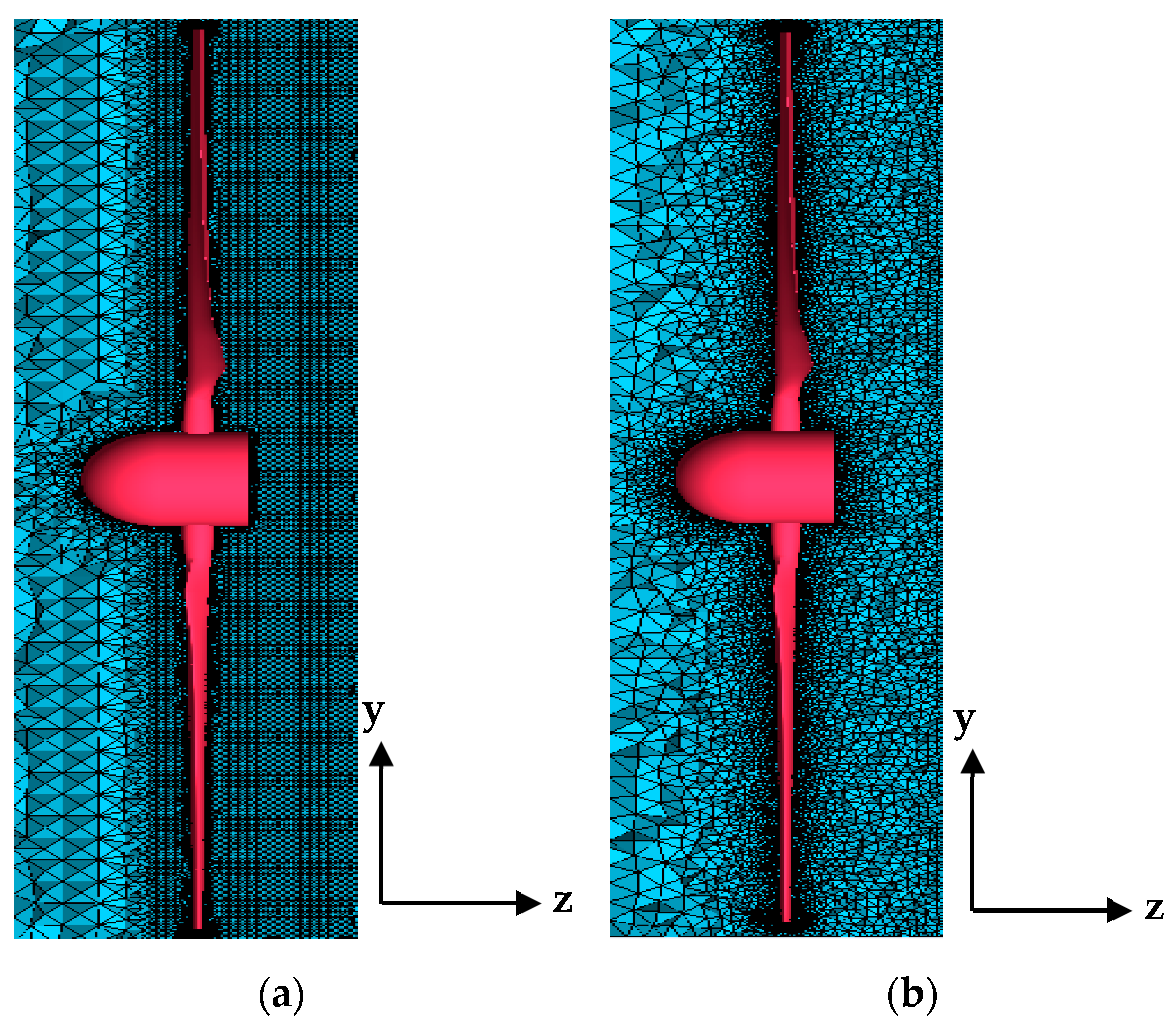
3.1. Mesh Parameters and Sizing

At the first stage of the meshing process, sizing parameters were set using the advanced sizing function option in ANSYS 2023 R2 Meshing window software as proximity and curvature, aiming to densify the proximity and small proximity with fine relevance with high smoothing and minimum size 1.4599 × 10⁻². To avoid non-conformal mesh and negative volumes in which the nodes from inner and outer domains do not connect or match to each other, a new part was defined that combines the inner and outer domains with connections and contacts. To densify the nodes around the airfoil, since it experiences the highest disturbance, it is mandatory to conduct an edge sizing along the upper and lower edges of the airfoil based on the number of divisions chosen to be 200 with hard behaviour and activated bias option of 3. Furthermore, inflation is necessary in this process which adds structural layers along the edges and performs a gross rate to resolve the boundary layer. The inflation shown in Figure 4 is done along the three edges of the airfoil with first layer height (y+) obtained from the Pointwise CFD tool and determined by 1.23 × 10⁻⁵ m with low y+. In this step, a single y+ value of 33 was chosen for all turbulence models, including k-epsilon and k-omega, based on practical considerations. While lower y+ values are ideal for some models (e.g., y+ < 1 for k-omega), using a higher y+ value like 33 is often acceptable for capturing flow behaviour, particularly in the context of the k-epsilon model, which performs well with y+ values in the range of 30–500 [34].

To verify the relationship between growth rate and meshing quality, various growth rates were used as presented in

Table 2. Meshing growth rate and meshing quality.

Skewness		Orthogonal Quality
Growth Rate	Meshing Metrics	Growth Rate	Meshing Metrics
1.05	0.43	1.05	0.67
1.04	0.38	1.04	0.71
1.03	0.31	1.03	0.78
1.02	0.24	1.02	0.86

and compared in

Table 3. Skewness and orthogonal quality meshing statistics references.

Skewness
Excellent	Very Good	Good	Acceptable	Bad	Unacceptable
0–0.25	0.25–0.50	0.50–0.80	0.80–0.94	0.94–0.97	0.97–1.00
Orthogonal Quality
Unacceptable	Bad	Acceptable	Good	Very Good	Excellent
0–0.001	0.001–0.14	0.14–0.20	0.20–0.64	0.64–0.95	0.95–1.00

. It is observed that the validation of the growth rate and statistical parameters such as skewness are crucial in defining the meshing quality. Furthermore, it was validated that the meshing qualities obtained were excellent and very good in skewness and orthogonal quality meshing statistics, respectively, as shown in Table 2. Hence, a 1.02 growth rate was selected in this case.

3.2. Mesh Topological Tolerence

The Robust Octree algorithm, while efficient and consistent in its mesh creation, frequently lacks the appropriate level of detail required for complex geometries, resulting in reduced topological tolerance. By contrast, the Quick Delaunay approach exhibits greater topological tolerance by producing a more precise mesh that closely matches the curved surfaces of the airfoil. By accurately capturing the intricate geometric features, this approach enables improved resolution of the boundary layer and crucial aerodynamic processes like flow separation and vortex development. The implementation of smoother mesh transitions, where the gradual ratio is set at 1.2, allows the mesh to adjust to variations in geometry while maintaining the precision of the simulation. By increasing topological tolerance, the Quick Delaunay approach greatly decreases skewness and enhances orthogonal quality, guaranteeing that the computational fluid dynamics (CFD) simulations yield dependable and precise results that align with experimental predictions.

Figure 5 depicts the topological tolerance implemented in two distinct meshing algorithms, namely Robust Octree and Quick Delaunay, within the framework of mesh generation. Topological tolerance pertains to the capacity of the mesh to adjust to the fundamental geometry, precisely capturing important surface details and flow characteristics while preserving the integrity of the mesh structure. Ensuring surface accuracy and correct boundary layer resolution is crucial when simulating intricate geometries like the S809 airfoil. For more case details,

Table 4. Three-dimensional case list of considered parameters and their values.

Input Parameter	Value/Type
Angle of attack	$3^{\circ }$
Kinematic viscosity	$1.7894\times {10}^{-5}$
Solution method	Second order upwind
Length	1 m
Solver type	Pressure-based
Turbulent intensity	5%
Input parameter	Magnitude
Density of fluid	1.225 $\mathrm{k}\mathrm{g}/{\mathrm{m}}^3$
Viscous model	k-omega SST
Operating pressure	0 gauge (1 atm)
Operating temperature	288.16 K
Velocity flow	5–10 m/s
Time	Steady
Turbulent viscosity ratio	10

tabulates the considered parameters in the three-dimensional case.

3.3. Mesh Independence Study

The mesh independence study, as illustrated in Figure 6 and

Table 5. Meshing number of cells and torque generation.

Mesh No.	No. Cells (Millions)	Torque (N-m)	Error (%)
M1	11.010	780.25	29.09
M2	11.280	829.30	24.61
M3	11.985	917.60	16.58
M4	13.027	1023.15	6.99
M5	12.662	973.80	11.50
Exp. [35]	ــــــــــــــــــ	1100	ــــــــــــ

, investigates the influence of different mesh densities on the projected torque for the NREL Phase VI rotor. The objective of the study is to determine the most effective arrangement of mesh that achieves a balance between accuracy and computational efficiency. Figure 6 displays five mesh configurations (M1 to M5) with cell counts that increase gradually. The evaluation of these configurations is based on their capacity to forecast the torque at a wind speed of 8 m/s, with a specific emphasis on the precision of the outcomes in comparison to experimental data. The data emphasize that using finer meshes, particularly M4 and M5, results in lower error percentages, indicating enhanced accuracy in capturing the intricate flow dynamics around the rotor blades, such as boundary layer separation and vortex shedding.

Additionally, the error percentage was calculated by comparing the simulated torque values with the experimental torque value of 1100 N-m [35]. Table 4 presents a comprehensive analysis of the mesh configurations, including the number of cells, torque predictions, and error percentages in relation to the experimental torque of 1100 N-m. The mesh with the finest resolution, M4, consisting of 13.027 million cells, exhibits the lowest error rate of 6.99%. In contrast, coarser meshes such as M1 and M2 yield significantly higher error rates of 29.09% and 24.61%, respectively. This highlights the significance of mesh refinement in attaining dependable and accurate computational fluid dynamics (CFD) forecasts, especially in accurately representing aerodynamic forces. The results validate that the density of the mesh is crucial in determining the accuracy of computational fluid dynamics (CFD) simulations. Despite the increased computational costs, the use of finer meshes, specifically M4 and M5, is justified by their enhanced accuracy in predicting torque. In order to achieve precise evaluations of wind turbine aerodynamic performance, it is imperative to use meticulously developed meshes. This ensures that the simulation results closely match the experimental data, thereby increasing the study’s reliability.

4. Results and Discussion

In this section, the results of the 2D and 3D simulations are presented. Furthermore, the wake effect is also addressed and assessed using the Gaussian model which assumes the highest wind velocity deficit occurs always directly behind the turbine’s blade at an x = 0. The Gaussian model shapes a normal distribution or bell shape of statistics in which the wake occurs from the centreline of the shape to the rightward which is shown in Figure 7.

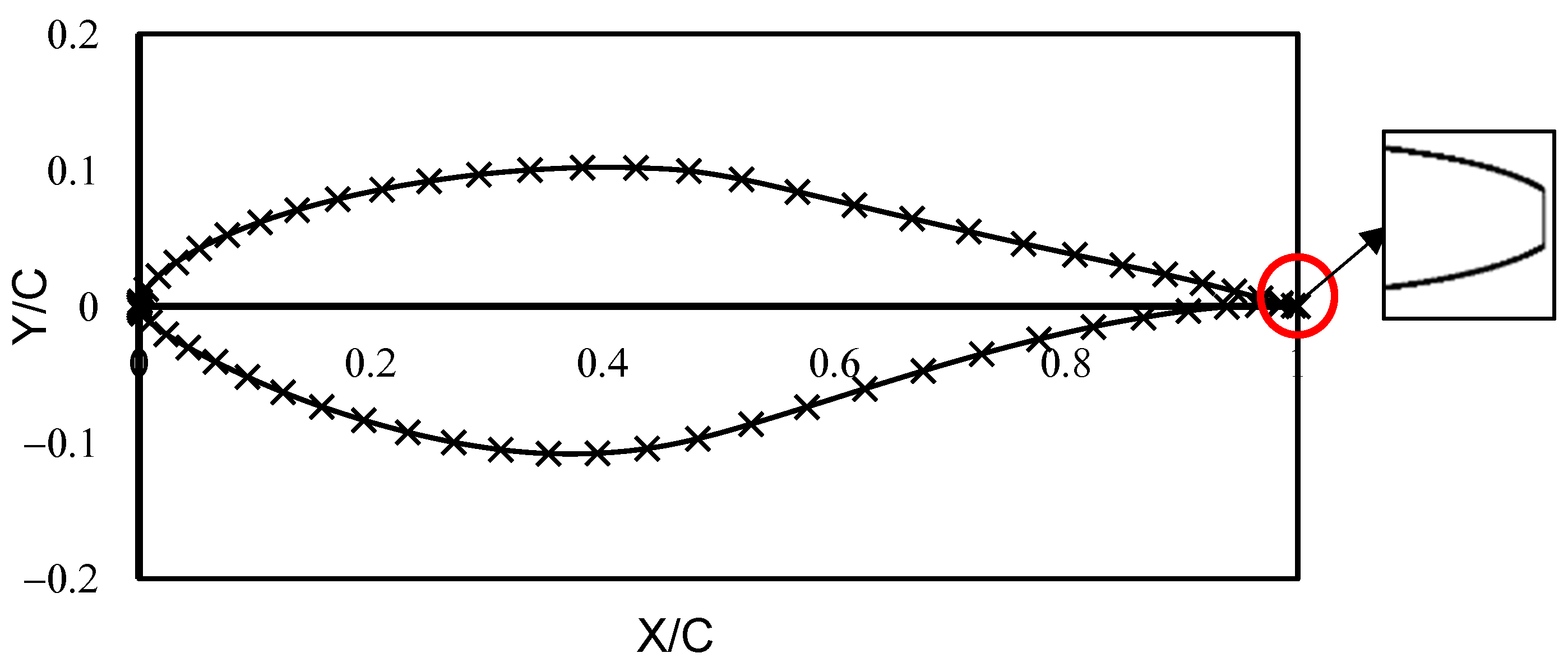
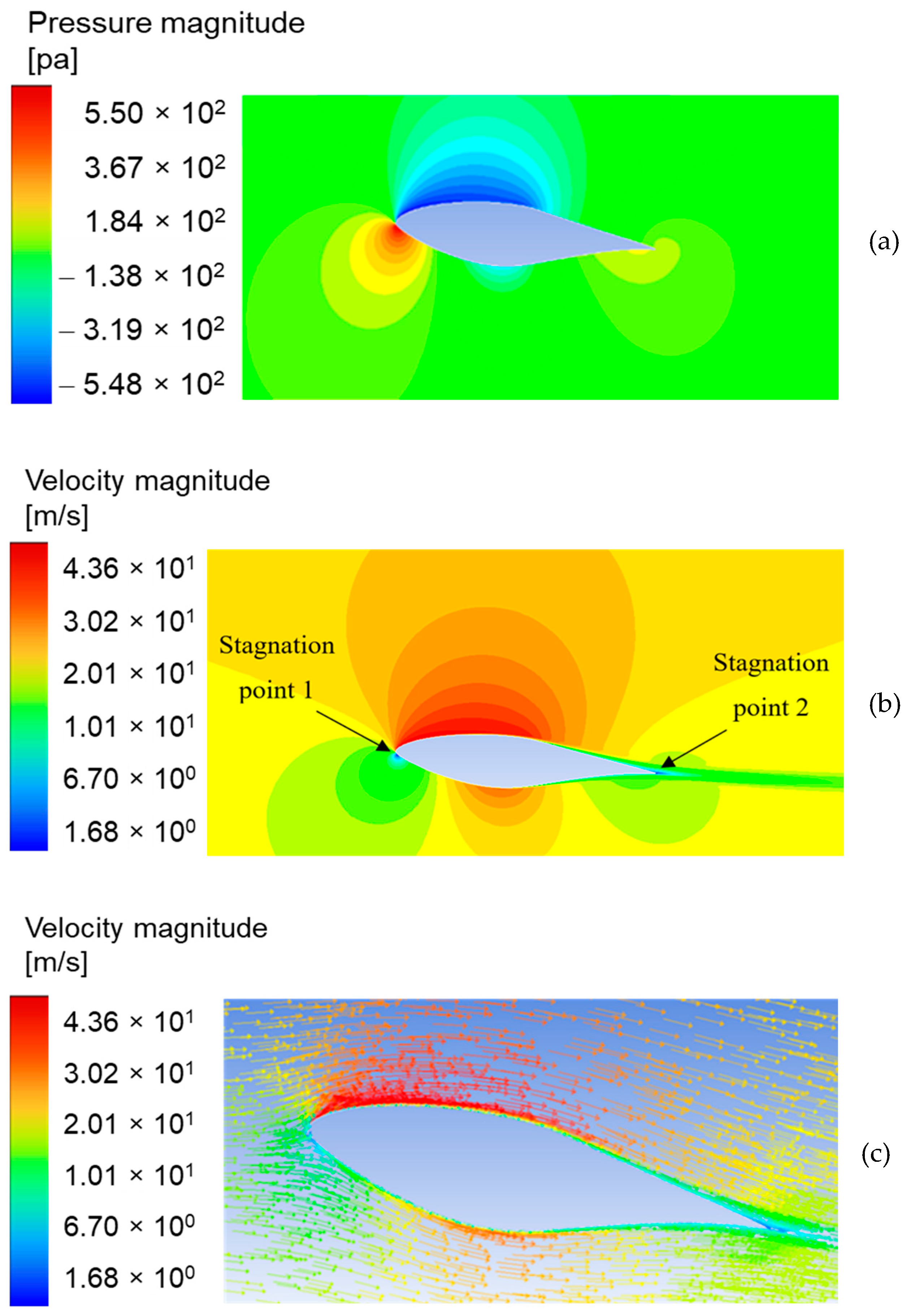
4.1. Two-Dimensional Analysis of S809 Airfoil

In the analysis of the S809 airfoil, Figure 8 in the analysis of the S809 aerofoil displays the pressure contours, velocity contours, and airflow vectors obtained from the two-dimensional computational fluid dynamics (CFD) simulation. These visualisations are crucial for comprehending the aerodynamic efficiency of the aerofoil. The pressure contours depicted in Figure 8a illustrate the distribution of pressure across the surface of the aerofoil. The regions near the stagnation point at the leading-edge exhibit higher pressure, while the upper surface displays lower pressure areas. This pattern is in line with the generation of lift. Figure 8b displays the velocity contours, which reveal areas of increased flow on the upper surface and decreased flow on the lower surface. This disparity in flow rates contributes to the necessary pressure difference for generating lift. The airflow vectors in Figure 8c clearly illustrate the direction and strength of the flow around the aerofoil, indicating regions where flow separation and recirculation may happen, which can affect the drag properties.

Expanding on this analysis, Figure 9 provides a numerical representation of the forces exerted on the aerofoil. It reveals a calculated lift force of 2492 N and a drag force of 120.6 N. The force values are directly correlated with the thrust and aerodynamic efficacy of the wind turbine blade. The lift force, propelled by the pressure differential illustrated in Figure 8, plays a crucial role in the overall performance, while the drag force affects the efficiency of energy conversion. The findings depicted in Figure 9 align with the anticipated outcomes for an aerofoil functioning under comparable circumstances, thereby strengthening the importance of the observed flow patterns illustrated in Figure 8. Precise forecasting of lift and drag is crucial for dependable thrust force computations, which aid in optimising rotor design to enhance energy capture. By substituting the values in Equation (5), the thrust force is found to be 2476.07 N. On the other hand, the thrust coefficient which represents the ratio of the axial force (thrust) produced by the turbine to the available kinetic energy in the wind stream, was approximated using Equation (7) below, where C_T is the thrust coefficient, while $\mathsf{\rho }$, A, and V are the density of air, swept area of the turbine, and wind speed, respectively. The thrust coefficient C_T of 1.696, calculated by combining Equations (7) and (8), reflects the axial force on the rotor blades and indicates efficient energy extraction. This value falls within the typical range of 0.8 to 2.0 for high-performance wind turbines, confirming the rotor’s effective power generation [36]. Additionally, the C_T value helps assess structural loads and validates the accuracy of the CFD model by comparing it with experimental data, supporting both the aerodynamic performance and the reliability of the simulations.

This choice balances accuracy with computational efficiency, a common trade-off in engineering simulations. Given the grid independence achieved in this study and the minimal impact of further mesh refinement on the results, the selected y+ value is justified as it ensures reliable results while optimizing computational resources; such moderate values are often sufficient for practical simulations. Additionally, the grid independence achieved in the study confirms the reliability of the chosen y+, as further mesh refinement did not significantly affect the results, supporting the use of this approach for the wind turbine analysis.

$${\mathrm{F}}_{\mathrm{T}}={\mathrm{F}}_{\mathrm{L}}\cos \left(\mathrm{\varnothing }\right)+{\mathrm{F}}_{\mathrm{d}}\mathrm{s}\mathrm{i}\mathrm{n}\left(\mathrm{\varnothing }\right)$$

(7)

$${\mathrm{C}}_{\mathrm{T}}={\displaystyle \frac{{\mathrm{F}}_{\mathrm{T}}}{\left(0.5\right)\left(\mathsf{\rho }\right)\left(\mathrm{A}\right)\left({\mathrm{V}}^2\right)}}$$

(8)

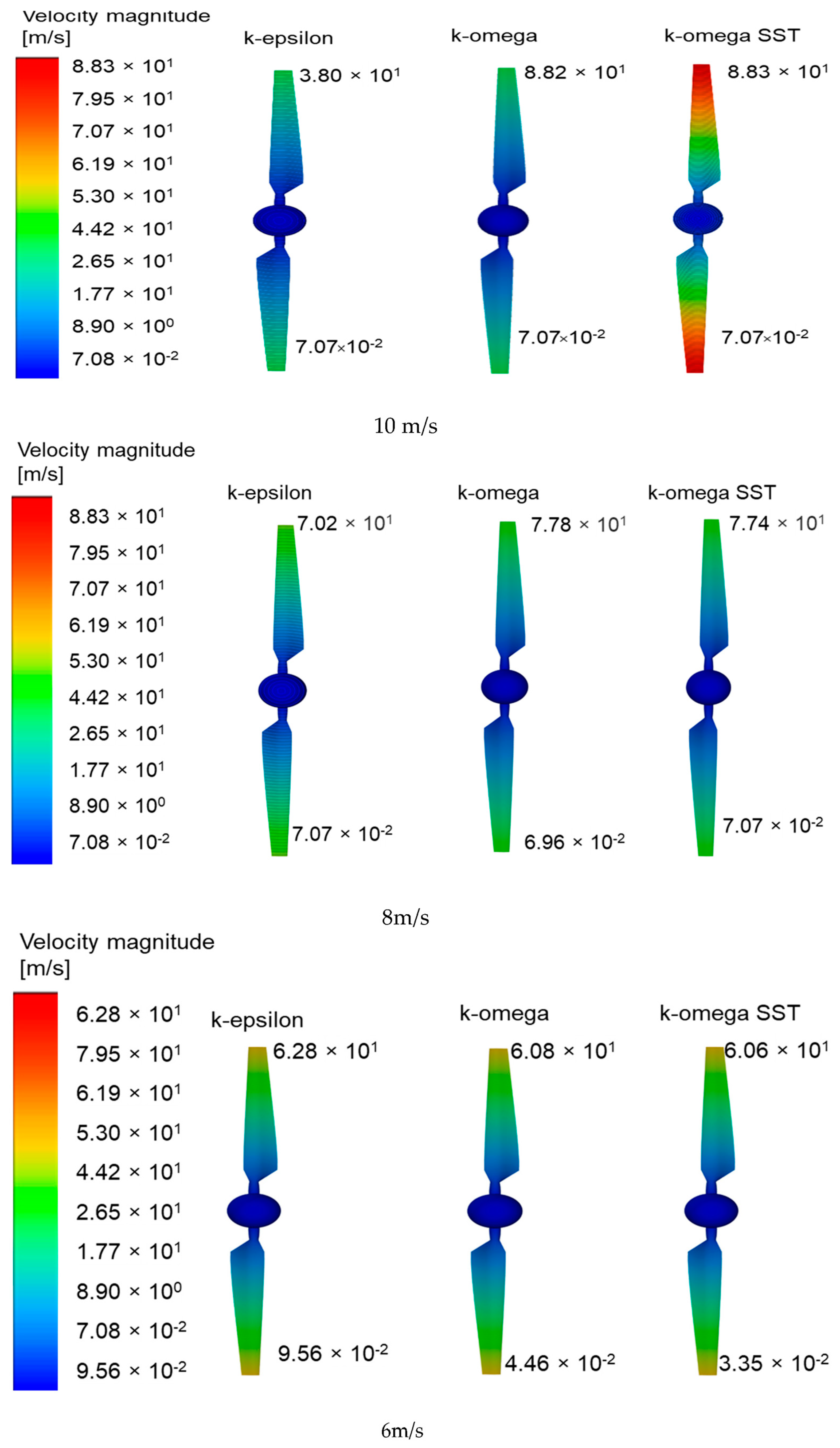
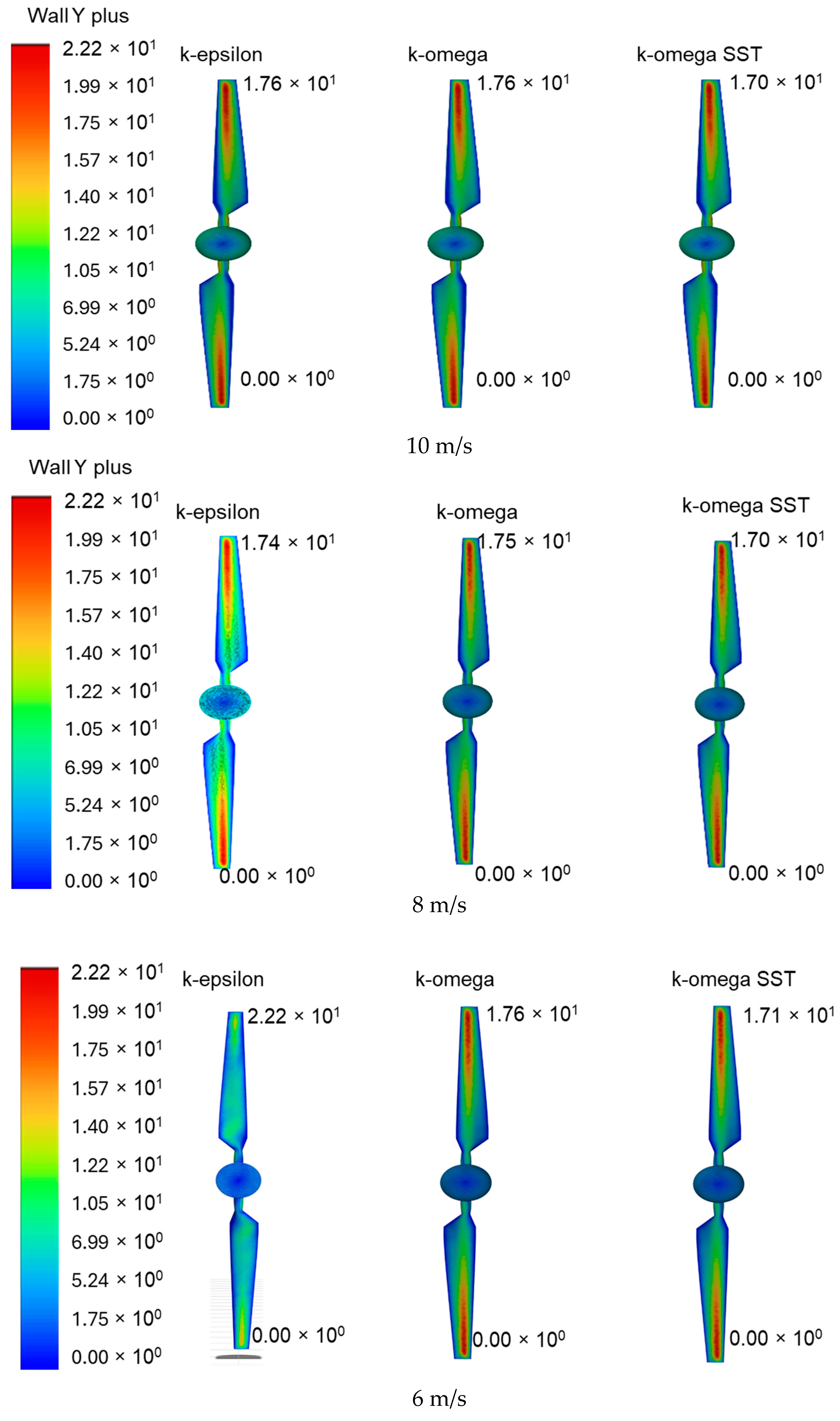
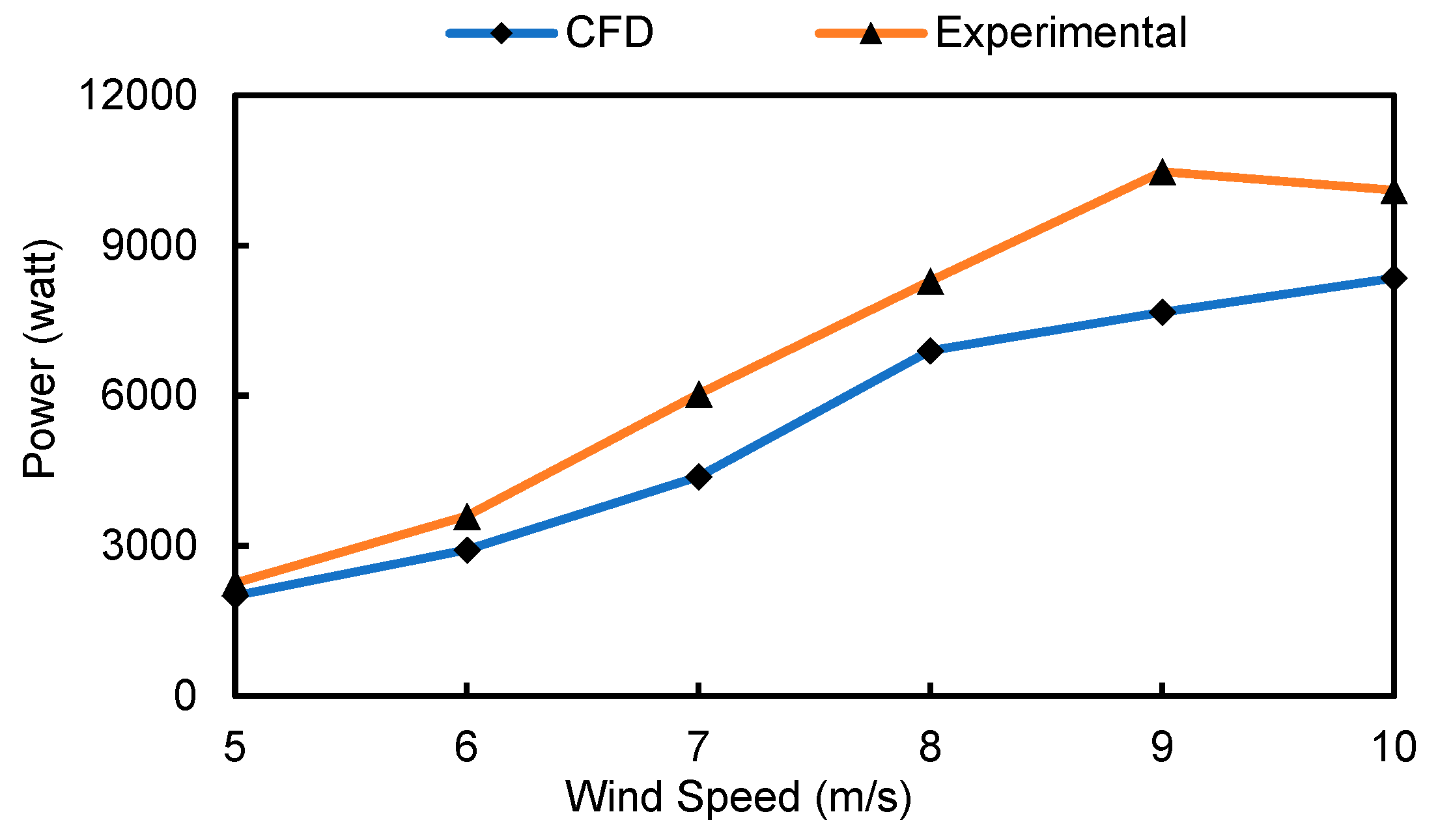
4.2. Three-Dimensional Analysis of NREL Phase VI Wind Turbine and Validation

The NREL Phase VI rotor was used to simulate three-dimensional flow at wind speeds of range (6–10 m/s). The simulation employed the k-epsilon, k-omega, and k-omega SST turbulence models, as shown in Figure 10, to generate particle pathlines. The particle pathlines illustrate the paths taken by airflow particles as they circulate around the rotor blades, providing a distinct visualisation of the aerodynamic behaviour in various flow conditions. The pathlines illustrate the intricate interplay between the airflow and the rotor surface, emphasising regions of flow detachment and reattachment in response to variations in wind speed. Particles ID in ANSYS refers to the unique identifiers for individual particles being tracked in the simulation, allowing the user to follow their specific trajectories and analyse their behaviour within the flow field where colours and their respected values are representing the number of the particle’s identifiers. High particle IDs do not indicate better or worse performance, but allow for detailed visualization of the flow behaviour over time, helping to analyse specific flow features around the rotor blades.

Figure 11 exhibits the simulation contours of the magnitude of velocity for the NREL Phase VI rotor at wind speeds of 10 m/s, 8 m/s, and 6 m/s, employing different turbulence models. The highest magnitude of velocity reaches 8.83 × 10 m/s, primarily at the edges of the blades, where the airflow speeds up because of rotational effects and influence. Conversely, the minimum velocity of 9.56 × 10⁻³ m/s is detected in close proximity to the rotor hub and in areas characterised by stagnation or recirculation, where the flow experiences a notable decrease in speed. The extreme values observed in this case represent the aerodynamic characteristics along the entire span of the rotor. High velocities at the blade tips indicate efficient energy extraction, while low velocities near the centre of the rotor suggest flow inefficiencies.

Across all turbulence models, the velocity contours display almost similar rates of transition from high velocities near the blade tips to lower velocities closer to the rotor hub. The maximum velocity occurs at the blade tips, driven by rotational speed and aerodynamic forces, while the lowest velocities are observed near the rotor’s centre and areas where flow stagnation or recirculation occurs. Despite the differences in turbulence models, the overall flow behaviour is consistent, showing effective energy extraction at the blade tips and regions of reduced flow near the hub. This similarity in contour patterns suggests that all models adequately capture the key flow features, such as acceleration at the blade tips and the slower-moving flow near the rotor’s centre.

Figure 12 illustrates the static pressure distribution around the NREL Phase VI rotor at wind speeds of 10 m/s, 8 m/s, and 6 m/s using different turbulence models. The windward side of the rotor blades, near the leading edge, experiences the greatest static pressure, while the leeward side, where airflow separates and accelerates, has the lowest pressure. The pressure disparities are vital for generating lift, as the regions of higher pressure greatly enhance the rotor’s aerodynamic effectiveness. The observed pressure values fall within the anticipated operational ranges for wind turbines, thereby verifying the efficient functioning of the rotor under these circumstances. The disparity in pressure across the rotor can be ascribed to disparities in how the turbulence models simulate the separation and reattachment of flow, which affects the precision of pressure forecasts across the surface of the blade.

Figure 13 presents the Y+ values of the rotor blades’ wall for identical wind speeds and turbulence models. The Y+ values span a range of approximately 30–500 [34], which is suitable for accurately representing the boundary layer flow in computational fluid dynamics (CFD) simulations. Regions of higher Y+ values are found near the leading edge and hub, where the aerodynamic forces and shear stresses are most concentrated. Conversely, lower Y+ values are observed near the blade tips. The Y+ distribution guarantees that the mesh resolution is adequate for precise predictions of the behaviour of flow near the wall, especially in accurately capturing the dynamics of the boundary layer. The congruity of these values with established turbulence model prerequisites affirms that the mesh configuration is suitable for both the k-epsilon and k-omega models employed in the analysis.

The wall shear stress distribution is shown in Figure 14, illustrating the variation of shear forces across the rotor surface at different wind speeds. The highest shear stress values are concentrated near the blade tips, where the velocity and aerodynamic forces are greatest, leading to higher tangential forces on the rotor surface. Lower shear stress is observed near the rotor hub and in areas of flow separation, where the airflow decelerates. These shear stress values fall within acceptable ranges for wind turbine operation, ensuring that the rotor is designed to handle the mechanical loads imposed by the airflow. Variations in the shear stress patterns are influenced by how each turbulence model captures near-wall flow behaviour, particularly in regions of separation and reattachment, affecting the distribution of forces across the blade surfaces.

Table 6. Torque comparison between experimental and CFD.

Turbulence Model	Wind Speed (m/s)	CFD Torque (N-m)	Exp. Torque (N-m) [35]	Error (%)
k-epsilon	10	1481.67	1340	−10.57
k-omega		846.83		36.80
k-omega (SST)		996.66		25.62
k-epsilon	9	1192.33	1390	14.22
k-omega		866.87		37.63
k-omega (SST)		991.80		28.64
k-epsilon	8	989.10	1100	10.08
k-omega		824.73		25.02
k-omega (SST)		1023.15		6.986
k-epsilon	7	638.70	800	20.16
k-omega		584.00		27.00
k-omega (SST)		520.38		34.95
k-epsilon	6	431.80	478	9.665
k-omega		387.01		19.03
k-omega (SST)		344.44		27.94

compares the torque values predicted by various CFD simulations with experimental torque measurements for the NREL Phase VI rotor across different wind speeds, revealing that the maximum torque predictions closely match experimental results, while minimum torque values show slight deviations, particularly at lower speeds. These discrepancies highlight the challenges faced by turbulence models in accurately capturing flow separation and complex aerodynamic behaviour. In parallel,

Table 7. Average CFD torque and power output validations with experimental results.

CFD Simulation
Rot. Speed	Wind Speed	Torque	Power	Cp	Error
rad/s	(m/s)	(n-m)	(m/s)	unitless	(%)
7.54	5	266	2006	0.329	7.54
7.54	6	387	2917	0.278	18.87
7.54	7	581	4380	0.262	27.38
7.54	8	915	6899	0.277	16.82
7.54	9	1017	7668	0.216	26.83
7.54	10	1108	8354	0.172	17.31
Experimental [35]
7.54	5	300	2262	0.371	-
7.54	6	477	3596	0.342	-
7.54	7	800	6032	0.361	-
7.54	8	1100	8294	0.333	-
7.54	9	1390	10,480	0.300	-
7.54	10	1340	10,103	0.210	-

validates the average CFD torque and power outputs against experimental data, showing that the maximum power outputs at higher wind speeds are consistent with the experimental results, indicating reliable energy conversion predictions. However, minor differences in the minimum power outputs at lower speeds reflect the sensitivity of the turbulence models to flow behaviour under varying conditions. Regarding the change of values when comparing Table 6 and Table 7, k-omega SST theoretically should perform better as it combines k-omega and k-epsilon turbulence models advantages in predicting the flow regardless of its distance from the wall, yet in this case, it requires higher wind velocity than 10 m/s to initiate the separation of flow and in counts the shear stress transients. Despite these variations, the overall agreement between the CFD predictions and experimental data confirms that the models perform within acceptable accuracy ranges for both torque and power outputs. In addition, the power coefficient C_p on the other hand is defined by Equation (10) which is how efficiently a turbine converts the energy in the wind to electricity. From Table 7, the highest achieved C_p was at 5 m/s wind speed with 0.37 at the experimental method. In terms of power outputs, Figure 15 shows simulated and experimental wind turbine power output. Moreover, torque values in Table 7 have been calculated by obtaining the average torque value of the three predicted turbulence models for each wind speed.

$$\mathrm{P}=\mathsf{\omega }\times \mathrm{T}$$

(9)

$${\mathrm{C}}_{\mathrm{p}}={\displaystyle \frac{\mathrm{A}\mathrm{c}\mathrm{t}\mathrm{u}\mathrm{a}\mathrm{l} \mathrm{w}\mathrm{i}\mathrm{n}\mathrm{d} \mathrm{t}\mathrm{u}\mathrm{r}\mathrm{b}\mathrm{i}\mathrm{n}\mathrm{e} \mathrm{p}\mathrm{o}\mathrm{w}\mathrm{e}\mathrm{r}}{\mathrm{M}\mathrm{a}\mathrm{x}\mathrm{i}\mathrm{m}\mathrm{u}\mathrm{m} \mathrm{w}\mathrm{i}\mathrm{n}\mathrm{d} \mathrm{t}\mathrm{u}\mathrm{r}\mathrm{b}\mathrm{i}\mathrm{n}\mathrm{e} \mathrm{p}\mathrm{o}\mathrm{w}\mathrm{e}\mathrm{r}}}$$

(10)

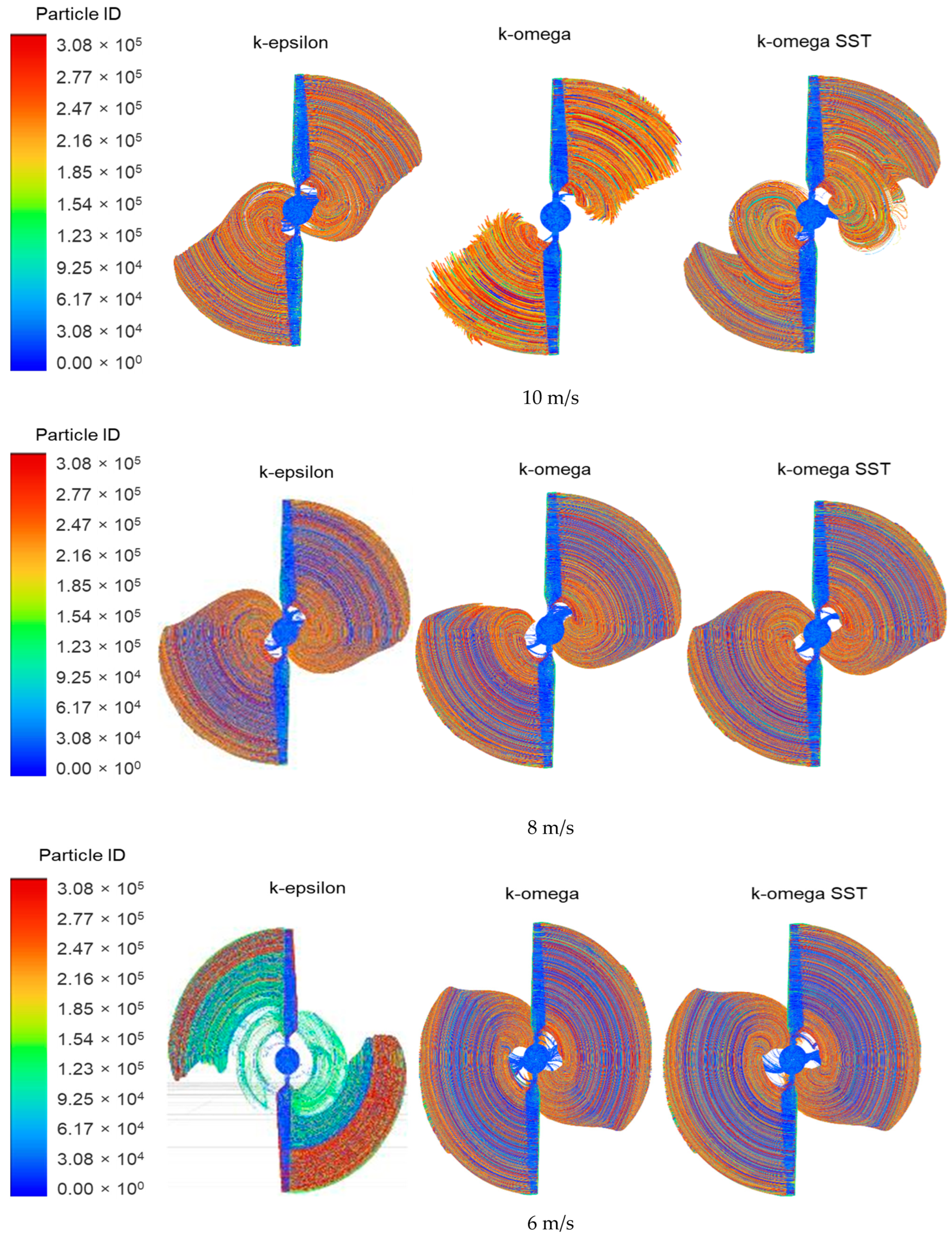
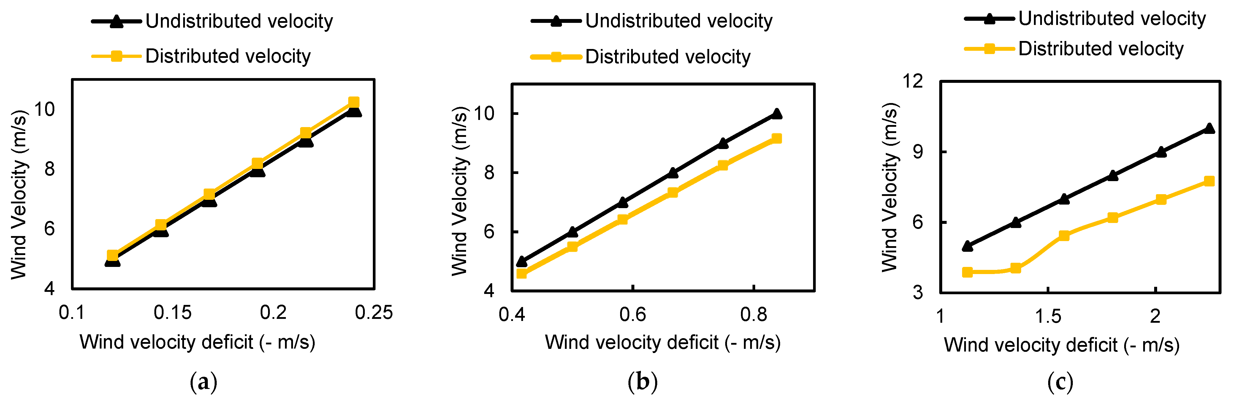
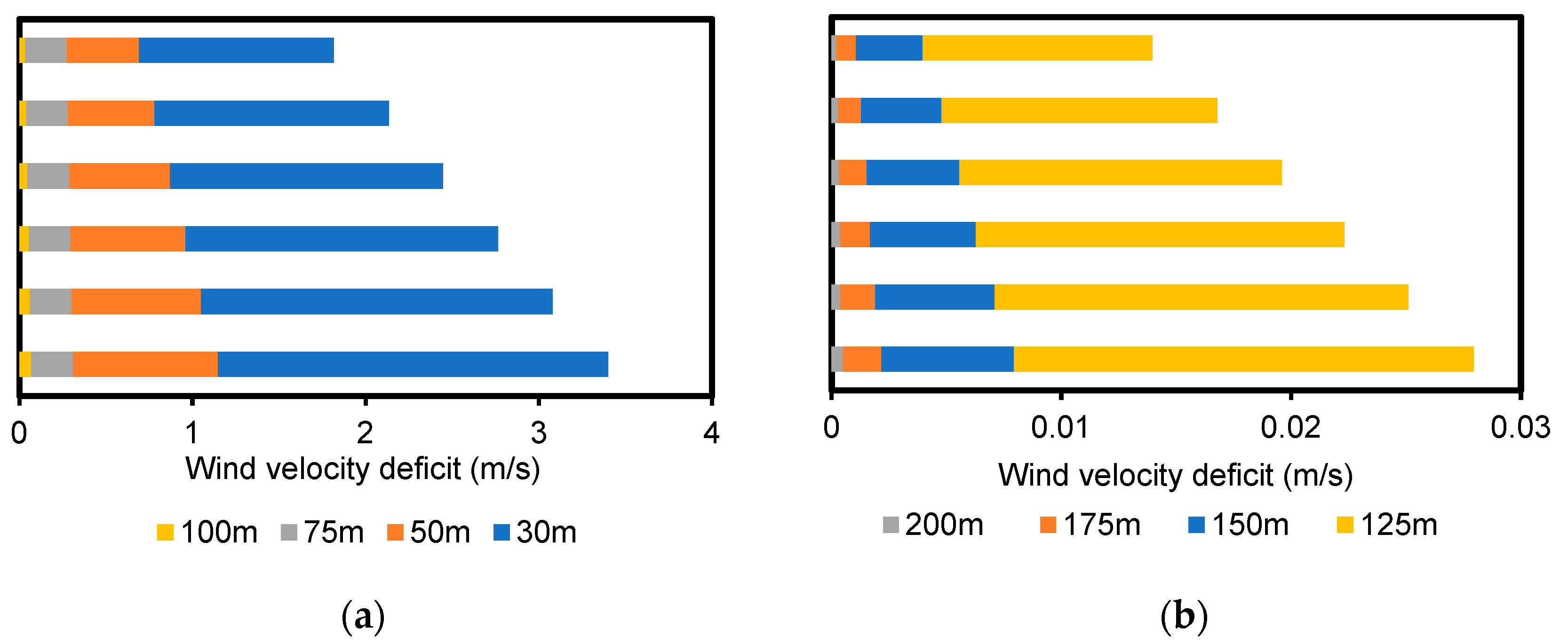
4.3. Local Wake Analysis Using the Gaussian Model

One of the most well-established wake assessment methods is the Gaussian model. As stated previously, the Gaussian model assumes the wind velocity deficit decreases exponentially from the centreline of the shape to the rightward. In other words, the highest wind velocity deficit occurs directly behind the blade of the turbine, where x = 0. For the current scenario, the assessment has been conducted at 8 different distances from the turbine. Figure 16 demonstrates the wind velocity deficit and a comparison between the distributed velocity and undistributed velocity which are the wind velocity behind the turbine that is disturbed due to the wake effect and the wind velocity before hitting the turbine blades, respectively. Figure 17, on the other hand, describes the wind velocity deficit concerning various values of x (distance) beginning with 30 m away behind the turbine, to 200 m. From the two figures, the highest wind velocity deficit always occurs close to the wind turbine which emphasizes the case in Gaussian model nature.

5. Conclusions

This study offers a comprehensive CFD analysis of the NREL Phase VI wind turbine, highlighting the importance of turbulence model selection for accurately predicting aerodynamic performance. By examining torque and power outputs across multiple wind speeds, the research identifies the k-epsilon turbulence model provided the closest match to the experimental data, particularly at higher wind speeds within the targeted range (6–10 m/s). Even though k-epsilon results had better agreement when validated with experimental data, theoretically k-omega (SST) should perform better as it combines k-epsilon and k-omega advantages in predicting the flow regardless of its distance from the wall. The study also emphasizes the significance of wake effects, which contribute to downstream velocity deficits that follow established exponential decay patterns.

The methodology involved detailed 2D and 3D simulations of the S809 airfoil, considering key aerodynamic forces such as lift and drag while incorporating a robust meshing strategy that ensured low skewness and high orthogonal quality. The accuracy of these simulations was validated through comparison with experimental results from NREL, confirming the reliability of the CFD approach used in this investigation.

This research addresses a critical gap in the understanding of turbulence models’ impact on wind turbine performance, particularly in the context of real-world applications. The insights gained from this study contribute to the optimization of wind turbine designs and provide practical recommendations for improving the accuracy of performance predictions. Overall, the results underline the necessity of careful turbulence model selection and wake effect consideration for advancing wind energy efficiency. These quantitative results provide critical insights for optimizing wind turbine performance, offering valuable contributions to the field of wind energy research. Airfoil parameters such as adding a cutting to the trailing edge of the airfoil will reduce drag and delay airflow separation. Other parameters to be considered for further research concerning S809 airfoil can be angle of attack and Rain and Droplet Impact in which droplets and rain can significantly degrade the aerodynamic performance of an airfoil by altering the boundary layer and causing premature separation. Experimental and numerical studies focusing on the interaction of the S809 airfoil with rain or other droplet impacts could provide insights into improving its robustness and performance under adverse weather conditions.

References

1. Ahmad, U.; Khan, M.A. Energy Demand in Pakistan: A Disaggregate Analysis Energy Demand in Pakistan: A Disaggregate Analysis. Pak. Dev. Rev. 2015, 47, 437–455. [Google Scholar] [CrossRef]
2. Conti-Ramsden, J.; Dyer, K. Materials innovations for more efficient wind turbines. Renew. Energy Focus 2015, 16, 132–133. [Google Scholar] [CrossRef]
3. Irfan, M.N.; Rosly, N. The Significant of Efficient Wind Turbines Arrangement in Mersing. Prog. Aerosp. Aviat. Technol. 2022, 2, 65–71. [Google Scholar] [CrossRef]
4. Samsudin, M.I.S.; Mohd, S. Development of A Small-Scale Vortex-Induced Wind Turbine. Prog. Aerosp. Aviat. Technol. 2022, 2, 10–18. [Google Scholar] [CrossRef]
5. Azam, S.R.S.; Malaysia, U.T.H.O.; Abidin, S.F.Z.; Ishak, I.A.; Khalid, A.; Mustaffa, N.; Taib, I.; Sukiman, S.L.; Darlis, N. Flow Analysis of Intake Manifold Using Computational Fluid Dynamics. Int. J. Integr. Eng. 2023, 15, 88–95. [Google Scholar] [CrossRef]
6. Kumar, B.; Srivastav, V.K.; Jain, A.; Paul, A.R. Study of numerical schemes for the CFD simulation of human airways. Int. J. Integr. Eng. 2019, 11, 32–40. [Google Scholar] [CrossRef]
7. Jamaludin, N.F.; Yusop, F.M.; Saji, N. Study Usage of Computational Fluid Dynamics (CFD) for Indoor Simulation. Prog. Eng. Appl. Technol. 2021, 2, 453–463. Available online: https://publisher.uthm.edu.my/periodicals/index.php/peat/article/view/799 (accessed on 28 September 2023).
8. Cleve, J.; Greiner, M.; Enevoldsen, P.; Birkemose, B.; Jensen, L. Model-based analysis of wake-flow data in the Nysted offshore wind farm. Wind Energy 2009, 12, 125–135. [Google Scholar] [CrossRef]
9. Sørensen, J.N.; Shen, W.Z. Numerical modeling of wind turbine wakes. J. Fluids Eng. Trans. ASME 2002, 124, 393–399. [Google Scholar] [CrossRef]
10. Neiva, A.; Guedes, V.; Massa, C.L.S.; Davy, D. Bello de Freitas a Review of Wind Turbine Wake Models for Wind Park Optimization; Brazilian Association of Mechanical Engineering and Sciences: Rio de Janeiro, Brazil, 2019; Available online: https://www.researchgate.net/publication/334330334 (accessed on 28 September 2023).
11. Tian, L.; Zhu, W.; Shen, W.; Zhao, N.; Shen, Z. Development and validation of a new two-dimensional wake model for wind turbine wakes. J. Wind Eng. Ind. Aerodyn. 2015, 137, 90–99. [Google Scholar] [CrossRef]
12. Kontou, M.G.; Asouti, V.G.; Giannakoglou, K.C. DNN surrogates for turbulence closure in CFD-based shape optimization. Appl. Soft Comput. 2023, Volume 134, 110013. [Google Scholar] [CrossRef]
13. Shakoor, R.; Hassan, M.Y.; Raheem, A.; Wu, Y.K. Wake effect modeling: A review of wind farm layout optimization using Jensen’s model. Renew. Sustain. Energy Rev. 2016, 58, 1048–1059. [Google Scholar] [CrossRef]
14. Katic, I.; Højstrup, J.; Jensen, N.O. A Simple Model for Cluster Efficiency Publication Date. In Proceedings of the European Wind Energy Association Conference and Exhibition, Rome, Italy, 7–9 October 1986; Volume 1, pp. 407–410. Available online: https://backend.orbit.dtu.dk/ws/portalfiles/portal/106427419/A_Simple_Model_for_Cluster_Efficiency_EWEC_86_.pdf (accessed on 6 October 2023).
15. Tian, L.; Zhu, W.; Shen, W.; Song, Y.; Zhao, N. Prediction of multi-wake problems using an improved Jensen wake model. Renew. Energy 2017, 102, 457–469. [Google Scholar] [CrossRef]
16. Jensen, N.O. A Simple Model for Cluster Efficiency; European Wind Energy Association: Etterbeek, Belgium, 1983. [Google Scholar]
17. Jensen, N.O. A Note on Wind Generator Interaction; Riso National Laboratory: Roskilde, Denmark, 1987; Volume 1. [Google Scholar]
18. Göçmen, T.; Van Der Laan, P.; Réthoré, P.E.; Diaz, A.P.; Larsen, G.C.; Ott, S. Wind turbine wake models developed at the technical university of Denmark: A review. Renew. Sustain. Energy Rev. 2016, 60, 752–769. [Google Scholar] [CrossRef]
19. Larsen, G.C. A Simple Wake Calculation Procedure; Risø-M, No. 2760; Risø National Laboratory: Roskilde, Denmark, 1988; p. 58. Available online: http://orbit.dtu.dk/ws/files/55567186/ris_m_2760.pdf (accessed on 28 September 2023).
20. Farndsen, S. Analytical modelling of wind speed deficit in large offshore wind farms. Wiley Intersci. 2006, 9, 39–53. [Google Scholar] [CrossRef]
21. Bastankhah, M.; Porté-Agel, F. A new analytical model for wind-turbine wakes. Renew. Energy 2014, 70, 116–123. [Google Scholar] [CrossRef]
22. Ghaisas, N.S.; Archer, C.L. Geometry-based models for studying the effects of wind farm layout. J. Atmos. Ocean Technol. 2016, 33, 481–501. [Google Scholar] [CrossRef]
23. Menter, F.R. Two-equation eddy-viscosity turbulence models for engineering applications. AIAA J. 1994, 32, 1598–1605. [Google Scholar] [CrossRef]
24. Calaf, M.; Meneveau, C.; Meyers, J. Large eddy simulation study of fully developed wind-turbine array boundary layers Large eddy simulation study of fully developed wind-turbine array. AIP Phys. Fluid 2013, 22, 015110. [Google Scholar] [CrossRef]
25. Barthelmie, R.J.; Pryor, S.C.; Frandsen, S.T.; Hansen, K.S.; Schepers, J.G.; Rados, K.; Schlez, W.; Neubert, A.; Jensen, L.E.; Neckelmann, S. Quantifying the impact of wind turbine wakes on power output at offshore wind farms. J. Atmos Ocean Technol. 2010, 27, 1302–1317. [Google Scholar] [CrossRef]
26. Barthelmie, R.J.; Frandsen, S.T.; Rathmann, O.; Hansen, K.S.; Politis, E.; Prospathopoulos, J.; Schepers, J.G.; Rados, K.; Cabezón, D.; Schlez, W.; et al. Flow and Wakes in Large Wind Farms: Final Report for UPWIND WP8; no. Risø-R-1765 (EN); Danmarks Tekniske Universitet, Risø National Laboratory Roskilde: Lyngby, Denmark, 2011. [Google Scholar]
27. Menter, F.R.; Kuntz, M.; Langtry, R. Ten Years of Industrial Experience with the SST Turbulence Model Turbulence heat and mass transfer. Turbul. Heat Mass Transf. 2003, 4, 625–632. Available online: https://www.researchgate.net/publication/228742295 (accessed on 28 September 2023).
28. Andias, R.; Mohd, S.; Zulkafli, F.; Didane, D.H. Simulation study of wind turbine system for electric powered vehicle. Int. J. Integr. Eng. 2020, 12, 76–81. [Google Scholar] [CrossRef]
29. Jones, W.P.; Launder, B.E. The prediction of laminarization with a two-equation model of turbulence. Int. J. Heat Mass Transf. 1973, 5, 413–418. [Google Scholar] [CrossRef]
30. Launder, B.E.; Sharma, B.I. Application of The Energy-Dissipation Model of Turbulence of the Calculation of Flow Near a Spinning Disc. Lett. Heat Mass Transf. 1974, 1, 131–138. [Google Scholar] [CrossRef]
31. Wilcox, D.C. Turbulence Modelling for CFD 3rd Edition. 2006. Available online: http://www.dcwindustries.com (accessed on 12 June 2023).
32. Reynolds, W.C. Computation of Turbulent Flow; Department of Mechanical Engineering, Stanford University: Stanford, CA, USA, 1989. [Google Scholar] [CrossRef]
33. Wilcox, D.C. Formulation of the k-ω turbulence model revisited. AIAA J. 2008, 46, 2823–2838. [Google Scholar] [CrossRef]
34. Versteeg, H.; Malalasekera, W. An Introduction to Computational Fluid Dynamics; Pearson: London, UK, 2007; Volume 10. [Google Scholar]
35. Hand, M.M.; Simms, D.A.; Fingersh, L.J.; Jager, D.W.; Cotrell, J.R.; Schreck, S.; Larwood, S.M. Unsteady Aerodynamics Experiment Phase VI: Wind Tunnel Test Configurations and Available Data Campaigns; National Renewable Energy Lab. (NREL): Golden, CO, USA, 2001; pp. 27–28. [Google Scholar]
36. Manwell, J.F.; McGowan, J.G.; Rogers, A.L. Wind Energy Explained. Theory, Design and Application; WILEY: Hoboken, NJ, USA, 2009. [Google Scholar]
Figure 1. S809 airfoil with a cutting trailing edge.
Processes 12 01994 g001
Figure 2. Case description: (a) NREL phase VI rotor; (b) NREL phase VI blade; (c) description of S809 airfoil design parameters.
Processes 12 01994 g002
Figure 3. Two-dimensional analysis of S809 domains. (a) Inner domain; (b) outer domain.
Processes 12 01994 g003
Figure 4. S809 airfoil after the inflation.
Processes 12 01994 g004
Figure 5. Meshing algorithm: (a) Robust Octree; (b) Quick Delauney.
Processes 12 01994 g005
Figure 6. Meshing independence study.
Processes 12 01994 g006
Figure 7. Gaussian wake model distribution.
Processes 12 01994 g007
Figure 8. S809 airfoil simulation contours: (a) Pressure contour; (b) velocity contour; (c) airflow vectors.
Processes 12 01994 g008
Figure 9. S809 airfoil simulation contours: (a) Lift force (Fl) (N); (b) drag force (Fd) (N).
Processes 12 01994 g009
Figure 10. NREL phase VI rotor simulation contours of particle pathlines for 10, 8, and 6 m/s wind velocities at various turbulence models.
Processes 12 01994 g010
Figure 11. NREL phase VI rotor simulation contours of velocity magnitude for 10, 8, and 6 m/s wind velocities at various turbulence models.
Processes 12 01994 g011
Figure 12. NREL phase VI rotor simulation contours of static pressure magnitude for 10, 8, and 6 m/s wind velocities at various turbulence models.
Processes 12 01994 g012
Figure 13. NREL phase VI rotor simulation contours of wall Y+ for 10, 8, and 6 m/s wind velocities at various turbulence models.
Processes 12 01994 g013
Figure 14. NREL phase VI rotor simulation contours of wall shear stress for 10, 8, and 6 m/s wind velocities at various turbulence models.
Processes 12 01994 g014
Figure 15. Comparison between simulated and experimental wind turbine power.
Processes 12 01994 g015
Figure 16. Comparison in wake effect using Gaussian wake assessment model in terms of wind velocity (distributed and undistributed) and wind velocity deficit at various distances (x): (a) At (x = 30 m); (b) At (x = 50 m); (c) At (x = 75 m).
Processes 12 01994 g016
Figure 17. Comparison in wake effect using Gaussian wake assessment model for wind velocity deficit at various distances (x): (a) At (x = 30 m to x = 100 m); (b) At (x = 125 m to x = 200 m).
Processes 12 01994 g017