Low-Carbon Transformation of Polysilicon Park Energy Systems: Optimal Economic Strategy with TD3 Reinforcement Learning

Abstract

To achieve the low-carbon transition in polysilicon production, this study proposes and validates a low-carbon economic dispatch strategy for a renewable hydrogen production and storage system in polysilicon parks based by TD3 algorithm. The study uses XGBoost to construct a surrogate model that reflects the nonlinear physical characteristics of the electrolyzer. Through a comparative analysis of operating strategies in five scenarios and sensitivity assessments of key parameters, complemented by comparisons with dispatch results from the DDPG and DQN algorithms, the effectiveness of the coupled operating strategy for electrolyzers, energy storage, and hydrogen storage devices is fully validated. This highlights the critical role of the TD3 algorithm in strengthening the robustness of the energy system under double-end source-load uncertainties. The results show that batteries flexibly adjust to the time-of-use electricity price, and the coordinated operation of the hydrogen storage devices as well as electrolyzers stabilize the electrolyzer efficiency, reducing the total system cost by 0.027% compared to fixed condition equipment models. The TD3 algorithm shows significant advantages in optimized dispatch, reducing the average daily operating cost by 0.6% and 1.2%, respectively, compared to the DDPG and DQN algorithms, and reducing the carbon emission cost by 2.0% and 12.0%, respectively. A comprehensive analysis shows that the proposed model reduces daily carbon emissions by 29.3% compared to the original system, but also introduces cost pressure, mainly due to the high operating costs of renewable energy equipment such as solar panels. This study provides a practical solution for renewable energy management.

1. Introduction

In the face of mounting global environmental concerns, the People’s Republic of China has established ambitious targets to be achieved by the years 2030 and 2060, respectively: a carbon peak and carbon neutrality [1]. At present, the industrial sector is responsible for a substantial share of the nation’s carbon emissions, particularly energy-intensive enterprises that establish their own power plants to reduce production costs, resulting in persistently high carbon emissions [2]. Polycrystalline silicon, a crucial industrial raw material for the solar photovoltaic and semiconductor sectors, is predominantly produced via the modified Siemens process. This method entails high electricity costs and substantial hydrogen demand during the production process, thereby accentuating the challenges associated with energy consumption and carbon emissions. The polysilicon industry primarily utilizes a “coal-fired + purchased electricity” power supply model for hydrogen production, indicating a significant role that energy conservation and carbon reduction efforts play in promoting sustainable energy development. In this context, the development of new energy and hydrogen-related technologies offers opportunities for the low-carbon transition of the polysilicon industry. Energy-saving renovation in polysilicon parks currently focuses on optimizing process technologies, such as adjusting specific process parameters, enhancing equipment efficiency, improving byproduct recovery, and reducing waste gas and heat emissions [3,4] to reduce energy consumption. However, research on integrating renewable energy and hydrogen storage technologies for low-carbon energy system transformation in parks remains scarce.

The academic community has achieved a wealth of research outcomes in enhancing the economic, environmental, and reliability aspects of green hydrogen–electricity systems. Mohammed et al. [5] constructed a multi-objective optimization model for hybrid photovoltaic–hydrogen energy storage system by using an improved nondominated sequential genetic algorithm, effectively balancing the operation cost and environmental cost. Fang et al. [6] combined the hydrogen energy system with renewable energy generation, and used a multi-objective stochastic black hole particle swarm algorithm to optimize the day-ahead power scheduling to minimize the cost and environmental impact. Hong et al. [7] developed a segmented fuzzy control optimal scheduling model for wind–hydrogen systems, and solved for the optimal hydrogen production power through an artificial bee colony algorithm. Kafetzis et al. [8] developed a hybrid automaton algorithm, and proposed an isolated islanded microgrid energy management strategy to solve the operation optimization problem of renewable energy, battery, and hydrogen storage systems. Pu et al. [9] employed a stochastic delta Gray Wolf optimizer and a two-layer planning approach to address equipment aging and loads. Their findings indicated that the electricity–hydrogen–cooling–heating cogeneration system offers economic advantages in effectively managing degradation costs and the benefits of seasonal hydrogen storage. In addressing mixed-integer nonlinear stochastic optimization models, existing studies have predominantly utilized mathematical planning algorithms and heuristic algorithms. Mathematical programming is capable of identifying the global optimal solution; however, this is contingent upon the accuracy of model construction and data prediction. Consequently, it is inefficient for large-scale nonlinear and uncertain optimisation problems. Heuristic algorithms reduce the reliance on models and data; nevertheless, for high-dimensional problems, their convergence speed and generalisation ability are limited. Furthermore, the performance of heuristic algorithms is heavily dependent on the characteristics of the problem and specific instances.

The loads of electricity, hydrogen, and cooling during polysilicon production are influenced by material and temperature distribution, and they exhibit the same uncertainty and volatility as renewable energy output [10]. To address this problem, deep reinforcement learning (DRL) algorithms demonstrate significant potential in comparison to traditional optimization algorithms. DRL algorithms learn the optimal policy through the interaction between intelligences and the environment, without reliance on accurate mathematical models or complex data prediction, and they exhibit favorable anti-interference and generalization capabilities [11]. Among the extant studies, Shi et al. [12] used deep Q-networks to optimize the energy management of a hydrogen-electric coupled system to cope with demand-side uncertainty in smart grids. Zhang et al. [13] optimized a microgrid model containing hydrogen storage and batteries by DQN, providing a solution for the stability of the energy supply of a polysilicon park under off-grid conditions. Liu et al. [14] compared the different parameters of the DQN algorithm and Q-learning algorithm in a grid-connected multi-energy flow integrated energy system, with special consideration of the robustness of the scheduling strategy to weather and electricity price fluctuations, which significantly improves the stability of energy supply. However, the DQN algorithm’s support for a discretized action space imposes limitations on the range of actions available and the system’s accuracy. To address these limitations, the DDPG algorithm was developed to learn in both state and action spaces using a deep neural network function approximator. Huang et al. [15] proposed a hybrid action space algorithm that integrates parameterized Dueling DQN and DDPG. This approach was employed to effectively address the complex co-scheduling optimization problem in microgrids. In a related study, Xu et al. [16] demonstrated the optimal operation method based on the MADDPG in dealing with the effectiveness in operational optimization problems with complex uncertainties between sources and loads. Despite the DDPG algorithm’s significant advantages in dealing with continuous state vectors and action vectors, overestimation of the Q-value can lead to suboptimal strategies. In comparison with the aforementioned methods, the dual delay mechanism of TD3 effectively addresses the issue of overestimation of the value function and variance, thereby significantly enhancing the stability and performance of the strategy [17]. Ref. [18] compared four deep reinforcement learning algorithms for the energy system scheduling problem, and the simulation results substantiate the superiority of the TD3 algorithm on the training set, test set, and sensitivity analysis.

The extant literature has centered on the analysis and optimization of hydrogen energy flow in integrated energy systems, frequently treating the energy efficiency of equipment as a constant and ignoring the flexibility of equipment output. In fact, the conversion efficiency of hydrogen production equipment varies nonlinearly with the loading rate, and the modeling of electrolyzer operation characteristics is especially critical [19]. Reference [20] established the nonlinear relationship between the electrolyzer output voltage and current and Ma [21] modeled the three-state and power-current nonlinear characteristics of the electrolyzer monobloc. However, the variable operating condition model increases the difficulty of model solving, which is not conducive to efficient calculation. This study proposes an integrated energy system operation optimization strategy that accurately addresses the source-load uncertainty and equipment operation nonlinearity challenges in the polysilicon park. The proposed strategy integrates the processes of hydrogen production, storage, and utilization from renewable energy sources. It also constructs a refined energy system operation model and efficiently simulates the physical behavior of the electrolyzer under variable operating conditions with the help of the XGBoost agent model. The TD3 deep reinforcement learning algorithm is used to achieve the goals of minimizing operating costs and low carbon emissions, and to enhance the system’s adaptability and stability to fluctuations in supply and demand.

2. Dynamic Efficiency Model for Electrolyzer

2.1. Actual Engineering Model

An electrolyzer is an electrochemical device that facilitates a reaction by regulating the electrochemical potential of an electrode. The most common types of electrolyzed water for hydrogen production include alkaline, PEM (proton exchange membrane), solid oxide, and anion exchange membrane electrolyzers. While alkaline electrolyzers are the most widely used, they exhibit disadvantages such as high operating temperatures and extended start-up times. Conversely, PEM electrolyzers have emerged as a potential alternative, offering benefits such as reduced operating temperatures and expedited start-up times. The efficiency of the electrolyzer is influenced by various factors, including electrolyte concentration, reactant flow, and current and voltage. To elucidate the complex interplay among these factors, numerous mechanistic and regression models have been developed [22]. To address this need, this paper proposes an efficiency model for PEM electrolyzers, grounded in the understanding of how power and temperature influence efficiency [23].

The efficiency of an electrolysis cell can be categorized into two distinct components: voltage efficiency and current efficiency. Current efficiency, also referred to as Faradaic efficiency, signifies the ratio of the theoretical electrical consumption to the actual electrical consumption necessary to yield a specific product. Conversely, voltage efficiency denotes the relative magnitude of the theoretical decomposition voltage in relation to the actual cell voltage [24,25]. Large-scale electrolyzers are generally composed of multiple electrolysis cells connected in series, and the electrolysis voltage of a single cell can be subdivided into three components, i.e., the Nernst voltage, activation overpotential, and ohmic overpotential, which are expressed in Equations (1)–(4):

$$U_{cell}=U_N+U_{act}+U_{res}$$

(1)

$$\left\{\begin{array}{cc}\hfill & U_N=E_{an}-E_{cat}=E_{rev}^0+{\displaystyle \frac{R{T}_{cell}}{2F}}ln\left(\sqrt{{\displaystyle \frac{p_{an}}{p_0}}}·{\displaystyle \frac{p_{cat}}{p_0}}\right)\hfill \\ \hfill & E_{rev}^0=1.229-0.9\times {10}^{-3}(T_{cell}-298)\hfill \end{array}\right.$$

(2)

$$U_{act}={\displaystyle \frac{R{T}_{cell}}{\alpha zF}}ln{\displaystyle \frac{j}{j_0}}$$

(3)

$$\left\{\begin{array}{cc}\hfill & U_{res}=\left[r_0+{\displaystyle \frac{d_m{\delta }_m}{{\sigma }_m(T_{cell},a_{H_{2}O}^m)}}\right]j\hfill \\ \hfill & {\sigma }_m={(0.6877+a_{H_{2}O}^m)}^{3}exp\left(-{\displaystyle \frac{10440{\left(a_{H_{2}O}^m\right)}^{0.25}}{R{T}_{cell}}}\right)\hfill \end{array}\right.$$

(4)

where $U_{cell}$ is the electrolysis voltage of a single electrolysis cell, $U_N$ is the Nernst voltage, $U_{act}$ is the activation overpotential, $U_{res}$ is the ohmic overpotential, $E_{an},E_{cat}$ are the potentials of the anode and cathode, $E_{rev}^0$ is the standard electrode potential, R is the ideal gas constant, $T_{cell}$ is the temperature of the electrolysis cell, F is Faraday’s constant, $p_{an},p_{cat},p_0$ are the pressures at the anode, cathode, and under standard conditions, respectively, $\alpha$ is the charge transfer coefficient, z is the number of electron transfers, j is the current density, $j_0$ is the exchange current density, $r_0$ is the internal resistance, $d_m$ is the thickness of the membrane, ${\delta }_m$ is the thickness of the membrane, ${\sigma }_m$ is the conductivity of the membrane, and $a_{H_{2}O}^m$ is the activity of water in the membrane.

Voltage efficiency is represented by a two-stage function. When the electrolysis voltage is below the thermodynamic neutral voltage, the electrical energy consumed by electrolysis is entirely converted into chemical energy and the enthalpy of water vapor; in this stage, thermodynamic efficiency is used for calculation. When the electrolysis voltage exceeds the thermodynamic neutral voltage, voltage efficiency is used for calculation, as shown in Equations (5)–(7):

$${\eta }_{H_2,1}^p={\displaystyle \frac{\Delta H_{LHV}/\left(zF\right)}{(\Delta H_{LHV}+Q_{vap})/\left(zF\right)}}={\displaystyle \frac{U_{LHV}}{U_{LHV}+U_{vap}}}$$

(5)

$$U_{vap}={\displaystyle \frac{p_{H_{2}O}}{zF}}\left({\displaystyle \frac{1}{p_{H_2}^{cat}}}+{\displaystyle \frac{1}{2p_{O_2}^{an}}}\right)\Delta H_{vap}$$

(6)

$${\eta }_{H_2,2}^p={\displaystyle \frac{\Delta H_{LHV}/\left(zF\right)}{U_{cell}}}$$

(7)

where ${\eta }_{H_2,1}^p$ represents the first phase hydrogen production efficiency, $\Delta H_{LHV}$ represents the low heating value of hydrogen, $Q_{vap}$ is the heat of vaporization of water, $U_{LHV}$ is the voltage corresponding to the low heating value, $U_{vap}$ is the voltage associated with the vaporization of water, $p_{H_{2}O}$ is the partial pressure of water vapor, $p_{H_2}^{cat}$ is the partial pressure of hydrogen at the cathode, $p_{O_2}^{an}$ is the partial pressure of oxygen at the anode, $\Delta H_{vap}$ is the molar enthalpy of vaporization, and ${\eta }_{H_2,2}^p$ represents the second phase hydrogen production efficiency.

On the other hand, some hydrogen gas will diffuse through the proton exchange membrane to the anode and undergo a reverse reaction, meaning that not all of the current at the electrodes is used for water electrolysis, which is the Faradaic efficiency defined by Equations (8) and (9):

$${\eta }_{H_2}^F={\displaystyle \frac{(n_{H_2}^p-n_x)\Delta H_{LHV}}{n_{H_2}^p\Delta H_{LHV}}}=1-{\displaystyle \frac{j_x}{j}}$$

(8)

$$j_x\simeq 2\left[{\lambda }_{H_2}^{T}F{\displaystyle \frac{p_{H_2}^{cat}+p_{O_2}^{an}}{d_m{\sigma }_m}}+{\displaystyle \frac{2a_x}{d_m{\sigma }_m}}j\right]·exp\left[{\displaystyle \frac{E_m}{R}}\left({\displaystyle \frac{1}{T_{ref}}}-{\displaystyle \frac{1}{T_{cell}}}\right)\right]$$

(9)

where ${\eta }_{H_2}^F$ represents the Faradaic efficiency of hydrogen production, $n_{H_2}^p$ represents the theoretical moles of hydrogen produced, $n_x$ represents the moles of hydrogen that have diffused to the anode, $j_x$ represents the diffusion current density, ${\lambda }_{H_2}^T$ represents the transport coefficient of hydrogen, $a_x$ represents the exchange area of the anode, $E_m$ represents the activation energy, and $T_{ref}$ represents the reference temperature.

In summary, the efficiency of the electrolysis cell can be expressed by Equation (10):

$${\eta }_{ET}=min({\eta }_{H_2,1}^p,{\eta }_{H_2,2}^p)·{\eta }_{H_2}^F$$

(10)

where ${\eta }_{ET}$ represents the total efficiency of the electrolyzer.

The hydrogen production power of the elecrolyzer can be described by Equation (11):

$$H_{ET}=P_{ET}{\eta }_{ET}$$

(11)

where $H_{ET}$ represents the hydrogen production power of the electrolyzer, $P_{ET}$ represents the power input to the electrolyzer, and ${\eta }_{ET}$ represents the efficiency of the electrolyzer. In the fixed operation mode, the efficiency ${\eta }_{ET}$ is considered a constant. However, in the variable operation mode, the efficiency ${\eta }_{ET}$ varies with the load rate and operating temperature.

2.2. Surrogate Model

Considering the nonlinear characteristics of the electrolyser model under variable operating conditions and its frequent invocation in reinforcement learning algorithms, a surrogate model was introduced to improve computational efficiency. This model was constructed using the XGBoost algorithm, an efficient distributed gradient boosting library based on the Gradient Boosting framework. The main advantage of XGBoost is its ability to use a second-order Taylor expansion to approximate the changes in the loss function when searching for the extremum of the loss function. In addition, it incorporates regularization terms in the loss function to regulate the complexity of the model, thereby preventing the occurrence of overfitting.

To construct the surrogate model, the physical model of the electrolyser was used to generate one thousand data points per degree over the operating temperature range, accumulating ten thousand data points in total. These data were divided into a training set and a test set, with 80% used to train the XGBoost model and the remaining 20% used to evaluate the model’s performance. Through the training set, XGBoost learned the complex relationship between the electrolyser’s efficiency and operating parameters, thereby constructing the surrogate model. The introduction of the test set was to verify the accuracy and generalizability of the surrogate model to ensure its reliability on unseen data.

2.3. Result Analysis

2.3.1. Actual Engineering Model Analysis

Figure 1 illustrates the variation of PEM electrolyzer efficiency with power and temperature. The figure reveals three salient features. First, the efficiency reaches a maximum at 0.3 and exhibits a rapid decrease on the left side and a gradual decrease on the right side. Second, on the left side of 0.6, the efficiency increases with the increase of temperature, while on the right side of 0.6, the efficiency decreases with the increase of temperature. Thirdly, the electrolysis efficiency is affected by the temperature under the low-power condition and is influenced by the temperature under the high-power condition. The electrolysis efficiency is greatly affected by temperature at low power and little affected by temperature at high power. The underlying reason for the observed shift in efficiency can be attributed to the interplay between voltage efficiency, which decreases with increasing current density, and thermodynamic efficiency, which increases with current density. This interaction leads to a phase transition in efficiency, where it initially rises and then falls. When considered in conjunction with the actual production process, the pursuit of maximum efficiency, while commendable, results in an electrolyzer output that is suboptimal. This is due to the fact that the equipment utilization efficiency is low. Conversely, an excessively high load also results in a reduction in efficiency, which is not conducive to energy savings. Therefore, the electrolyzer in this system is predominantly operated near the temperature junction point to balance the relationship between output and efficiency.

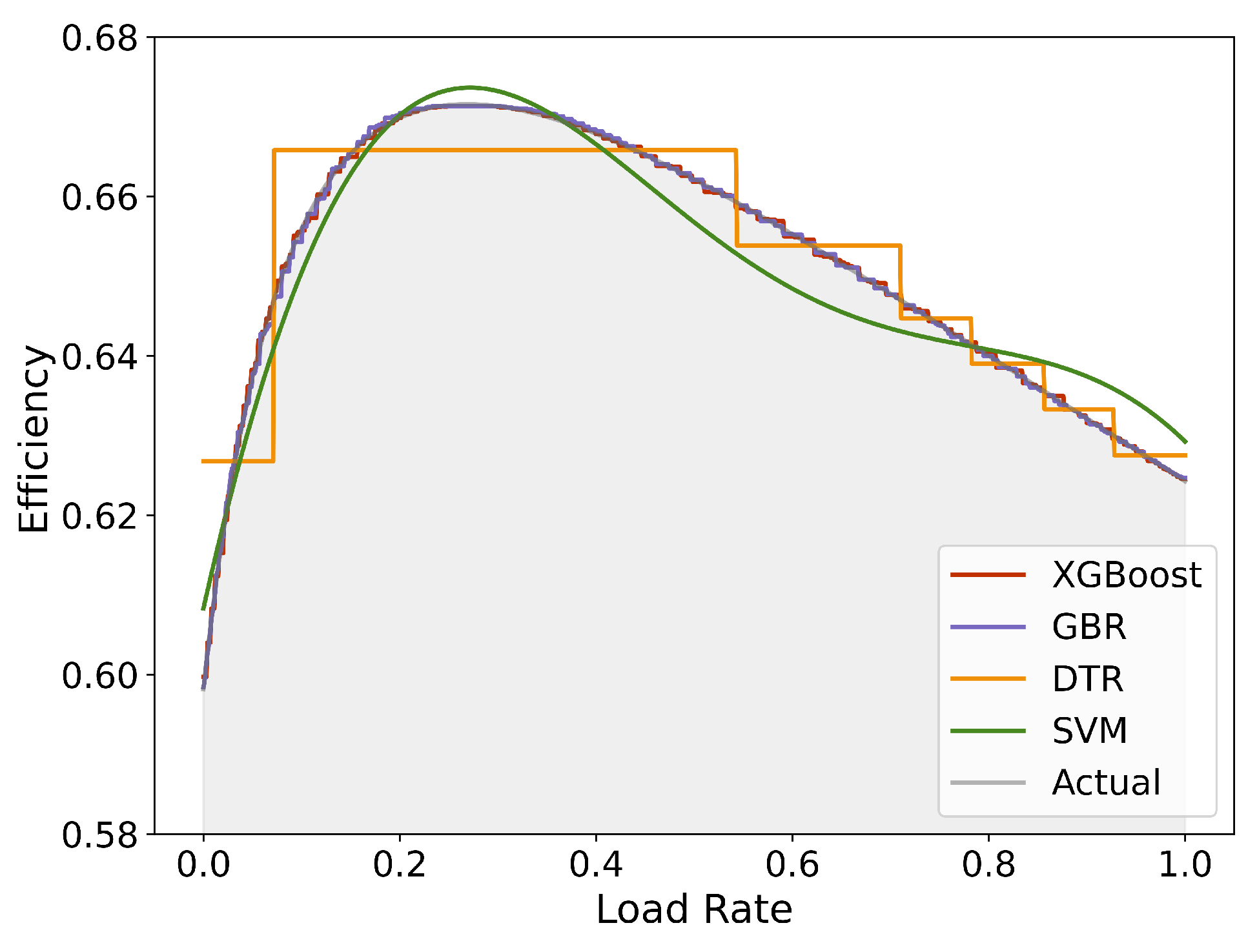
2.3.2. Surrogate Model Algorithm Comparison

In order to verify the robustness of the XGBoost models, they were compared with other agent modeling techniques. Figure 2 illustrates the fit of each model to the electrolyzer efficiency curve at its rated temperature. The mean square error (MSE) and coefficient of determination ($R^2$) on the entire dataset are presented in

Table 1. Goodness of fit comparison of different surrogate models.

Model	XGBoost	GBR	DTR	SVM
MSE	6.27 × 10−7	8.388 × 10−7	7.46 × 10−5	5.10 × 10−5
$R^2$	0.999	0.998	0.824	0.880

. The parameters of the XGBoost agent model are set to a maximum depth of the tree of 3, a learning rate of 0.2, and a number of iterations of 100. In contrast, the Support Vector Machine (SVM) uses a radial basis function kernel with parameters C of 100, gamma of 0.1, and epsilon of 0.01; Gradient Boosting Tree (GBR) has a learning rate of 0.1 and a maximum depth of 3; and Decision Tree (DTR) also has a maximum depth of 3. The test results show that XGBoost outperforms SVM, GBR, and DTR in two key metrics, $R^2$ and MSE, where XGBoost has an $R^2$ of 0.999 and an MSE of 6.27 × 10⁻⁷, while the other models perform relatively poorly. This outcome corroborates the efficacy and precision of XGBoost in electrolyzer efficiency prediction, thereby furnishing an efficient and accurate agent model for reinforcement learning algorithms and establishing the basis for addressing optimal operating efficiency.

3. Low-Carbon Economic Optimal Scheduling Model Based on TD3

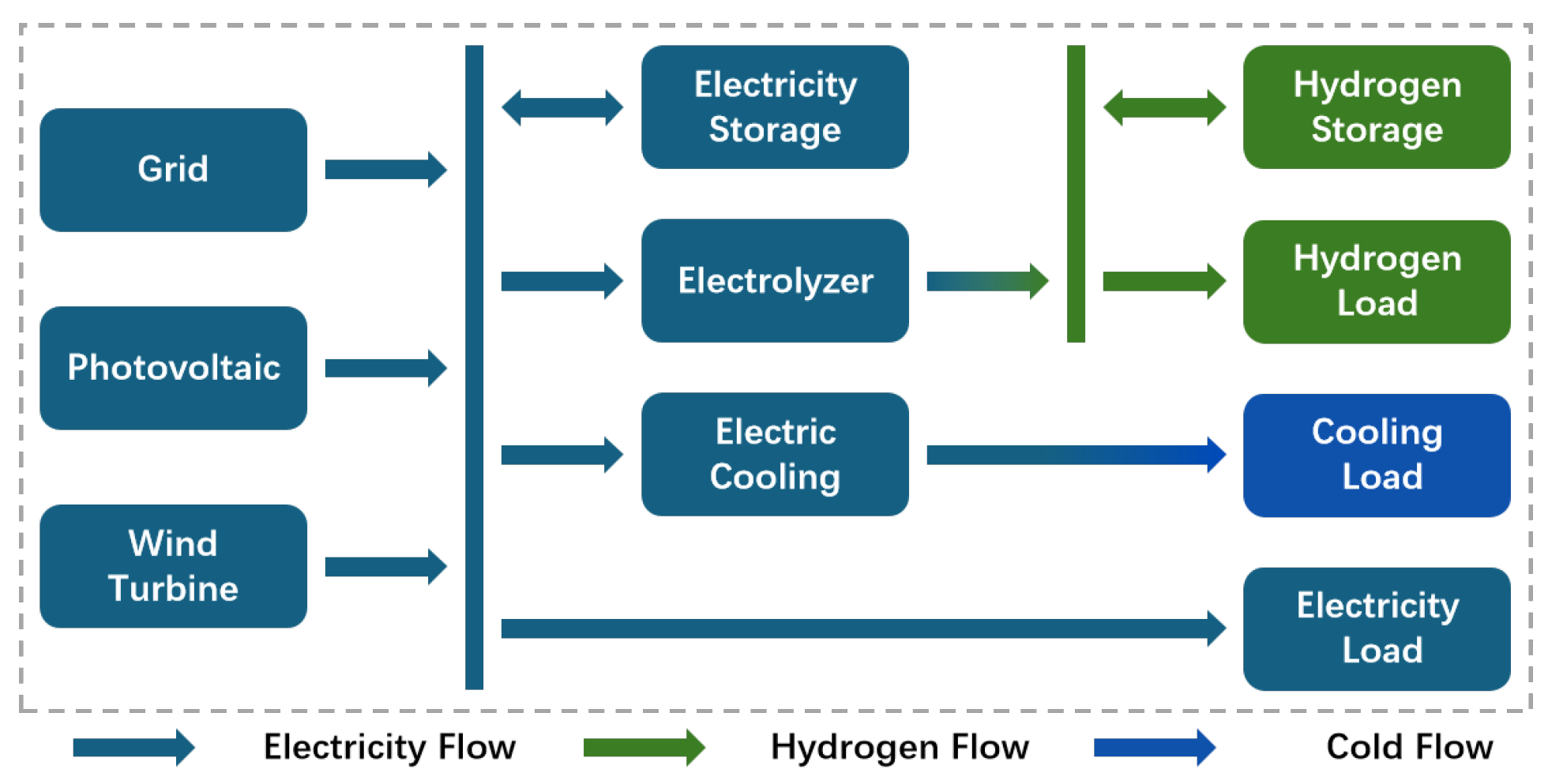
3.1. System Composition

The system under consideration is modeled after the design of a regional polysilicon plant, which necessitates hydrogen as a reducing agent during the reduction stage of trichlorohydrosilicon, refrigeration to maintain the normal temperature of the equipment, and electricity to supply the reduction furnace and other process equipment. Consequently, the system establishes an energy system consisting of three forms of energy: electric power, hydrogen, and cooling energy. The energy supply is derived from wind power and photovoltaic power generation, augmented by power procured from the higher power grid. The conversion link comprises two electrolyzer tanks for hydrogen production and one electric chiller for refrigeration. Energy storage entails hydrogen storage tanks and electric storage equipment. The production process encompasses three loads: electricity, hydrogen, and cooling. The collaboration between the new energy power plant and the superior power grid is instrumental in ensuring the continuity and stability of production. The system’s structural design is depicted in Figure 3. During daylight hours, when there is an abundance of new energy, the electric hydrogen generator operates at maximum capacity, producing hydrogen. The surplus hydrogen and electricity are then stored in the hydrogen storage tanks and the battery energy storage system, respectively. Conversely, during nocturnal hours or periods of insufficient renewable energy, the hydrogen storage tanks are given priority for hydrogen supply. In instances where hydrogen remains scarce, the electric hydrogen generator is utilized to augment hydrogen production. When a deficit of electric power arises, the system is supported by battery discharging or electricity procurement.

3.2. Objective Function

The low-carbon economic scheduling problem of the polysilicon park energy system involves the strategic adjustment of the output and operational status of various devices in the system at each time period, with the primary goal of meeting the production line load demand while minimizing the environmental impact. The evaluation indicators include the system’s operating costs, carbon emissions, and the hydrogen supply shortage rate. The objective function, which is central to this study, is designed to encapsulate these considerations and serves as the sole reward signal in the deep reinforcement learning algorithm used to train the intelligent agent. The objective function of the operational optimization model is expressed in Equation (12):

$$min\left(\sum _{t=1}^{24}\left(C_{\mathrm{grid},t}+C_{\mathrm{om},t}+HSS{R}_t\right)\right)$$

(12)

where $C_{\mathrm{grid},t}$ represents the electricity procurement cost at hour t, which includes both the electricity cost and the carbon emission cost, specifically calculated in Equation (13):

$$C_{\mathrm{grid},t}=P_{\mathrm{grid},t}\left(p_{\mathrm{grid}}+p_{\mathrm{co}2}\right)$$

(13)

where $P_{\mathrm{grid},t}$ is the electricity procured at hour t, $p_{\mathrm{grid}}$ is the time-of-use electricity price, and $p_{\mathrm{co}2}$ is the carbon emission cost.

The operational and maintenance cost of devices $C_{\mathrm{om},t}$ is anchored in the levelized unit energy cost of operation, as defined by Equation (14):

$$C_{\mathrm{om},t}=\sum _{i=1}^n\left(P_{i,t}·C_i^{\mathrm{OP}}\right)$$

(14)

For each device i, the levelized unit energy cost $C_i^{\mathrm{OP}}$ is meticulously calculated in Equation (15):

$$C_i^{\mathrm{OP}}={\displaystyle \frac{{\sum }_{y=1}^{Y_n}\left(C_y^{\mathrm{INV}}+C_y^{\mathrm{OM}}+C_y^D\right)/{(1+d)}^y}{{\sum }_{y=1}^{Y_n}\left(P_y/{(1+d)}^y\right)}}$$

(15)

where $C_y^{\mathrm{INV}}$ is the investment cost in year y, $C_y^{\mathrm{OM}}$ is the operation and maintenance cost in year y, $C_y^D$ is the depreciation cost in year y, d is the discount rate, and $Y_n$ is the service life of the equipment in years.

The depreciation cost $C_y^D$ is computed in Equation (16):

$$C_y^D={\displaystyle \frac{C_y^{\mathrm{INV}}{(1-d)}^{y-1}d}{1-{(1+d)}^{y-Y_n}}}$$

(16)

Hydrogen demand satisfaction is quantified by the hydrogen supply shortage rate $HSS{R}_t$, which is critical to ensure the reliability of the hydrogen supply chain, calculated in Equation (17):

$$HSS{R}_t=1-{\displaystyle \frac{P_{H_2,supply}}{H_{load,t}}}$$

(17)

where $P_{H_2,supply}$ is the hydrogen supply at hour t and $P_{H_2,\mathrm{load}}$ is the hydrogen demand at hour t.

3.3. Constraints

Energy balance constraints and equipment operation constraints need to be considered in the optimal operation model of the energy system in the polysilicon park. The operating constraints for the electrolyser have been presented in Chapter 2, and the energy balance constraints and other equipment operating constraints are presented below.

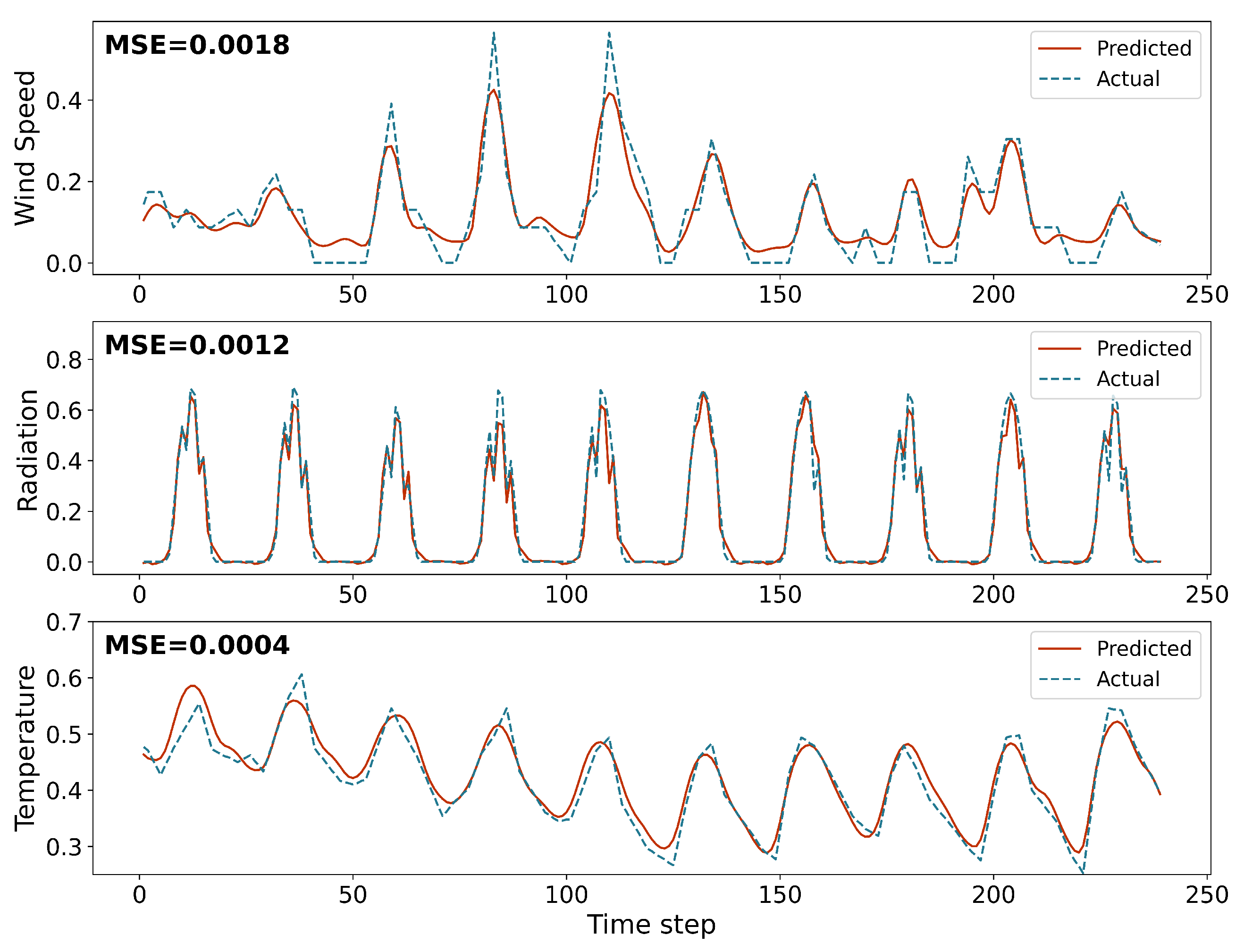
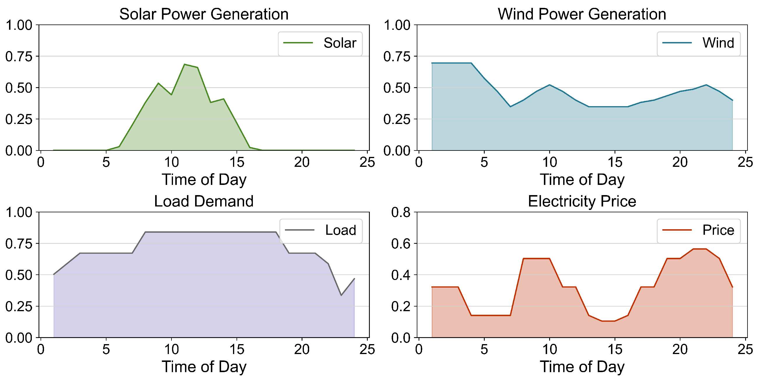
3.3.1. Photovoltaic Power Model

Photovoltaic systems use the photovoltaic effect to convert solar energy into electricity [26]. Their output power is directly proportional to light intensity and is affected by operating temperature. The power of the system can be approximated by Equation (18):

$$P_{PV}=f_{PV}{P}_{PV,rated}[1+{\alpha }_T(T_c-T_0)]G_t/G_0$$

(18)

where $P_{PV}$ represents the photovoltaic power generation, $f_{PV}$ represents the efficiency of the photovoltaic system, $P_{PV,rated}$ represents the rated power of the photovoltaic system, ${\alpha }_T$ represents the temperature coefficient, $T_c$ represents the operating temperature of the cell, $T_0$ represents the reference temperature, $G_t$ represents the actual light intensity, and $G_0$ represents the standard light intensity.

3.3.2. Wind Turbine Model

Wind turbines convert wind energy into mechanical energy by operating in the variable pitch constant power mode. They start at the cut-in wind speed, reach rated power as the wind speed increases, and maintain rated power by adjusting the pitch angle [27]. They stop when the wind speed exceeds the cut-off speed for safety reasons. The power generation of wind turbines can be estimated by Equation (19):

$$P_{WT}=\left\{\begin{array}{ccc}\hfill & 0\hfill & \hfill v<v_{in}orv>v_{out}\\ \hfill & {\displaystyle \frac{P_{WT,rated}(v_t-v_{in})}{v_r-v_{in}}}\hfill & \hfill v_{in}\le v_t\le v_r\\ \hfill & P_{rated}\hfill & \hfill v_r\le vs.\le v_{out}\end{array}\right.$$

(19)

where $P_{WT}$ represents the wind power generation, $vs.$ represents the wind speed, $v_{in}$ represents the cut-in wind speed, $v_{out}$ represents the cut-out wind speed, $v_t$ represents the rated wind speed, and $P_{WT,rated}$ represents the rated power of the wind turbine.

3.3.3. Energy Storage Model

The system includes hydrogen storage tanks and energy storage batteries. Hydrogen storage tanks compress hydrogen gas for dense storage, while energy storage batteries use secondary battery charge–discharge cycles to deliver electrical energy. Despite different principles and structures, both follow similar mathematical models, as shown by Equations (20) and (21):

$$\begin{array}{cc}\hfill P_{ES,t}& =P_{ES,t-1}-{\displaystyle \frac{P_{ES,dis,t}}{{\eta }_{ES,dis}}}+P_{ES,cha,t}{\eta }_{ES,cha}\hfill \end{array}$$

(20)

$$\begin{array}{cc}\hfill H_{HS,t}& =H_{HS,t-1}-{\displaystyle \frac{H_{HS,dis,t}}{{\eta }_{HS,dis}}}+H_{HS,cha,t}{\eta }_{HS,cha}\hfill \end{array}$$

(21)

where $P_{ES,t}$ represents the power of the energy storage at time t, $P_{ES,t-1}$ represents the power of the energy storage at the previous time step, $P_{ES,dis,t}$ is the power discharged from the energy storage, ${\eta }_{ES,dis}$ is the discharge efficiency of the energy storage, $P_{ES,cha,t}$ is the power charged into the energy storage, and ${\eta }_{ES,cha}$ is the charge efficiency of the energy storage. Hydrogen storage corresponds exactly to electricity storage.

For the two energy storage devices, there are not only capacity constraints but also rate constraints, which can be expressed in Equation (22):

$$\left\{\begin{array}{cc}\hfill & 0\le P_{ES,cha},P_{ES,dis}\le P_{ES,rated}\hfill \\ \hfill & C_{min}\le C_{ES}\le C_{max}\hfill \\ \hfill & P_{min}\le |P_{ES}|,|P_{HS}|\le P_{max}\hfill \\ \hfill & 0\le P_{HS,cha},P_{HS,dis}\le P_{HS,rated}\hfill \\ \hfill & H_{min}\le H_{HS}\le H_{max}\hfill \end{array}\right.$$

(22)

where $P_{ES,rated}$ represents the rated power capacity of the energy storage and $r_{ES}$ represents the ramp rate, which is the maximum rate at which the power output can change. Hydrogen storage corresponds exactly to electricity storage.

3.3.4. Electric Chiller Model

The electric chiller uses a compressor to pressurize and heat the refrigerant, which then releases heat in the condenser and changes phase to liquid. After pressure is reduced by the expansion valve, the liquid refrigerant evaporates in the evaporator, absorbing heat to provide cooling. The cooling capacity of the electric chiller is described by Equation (23):

$$C_{EC}=P_{EC}\left[{\zeta }_{EC,1}+{\zeta }_{EC,2}{\displaystyle \frac{P_{EC}}{P_{EC,rated}}}+{\zeta }_{EC,3}{\left({\displaystyle \frac{P_{EC}}{P_{EC,rated}}}\right)}^2+{\zeta }_{EC,4}{\left({\displaystyle \frac{P_{EC}}{P_{EC,rated}}}\right)}^3\right]$$

(23)

where $C_{EC}$ is the power of the electric chiller for cold production, $P_{EC}$ is the active power of the electric chiller, $P_{EC,rated}$ is the rated power of the electric chiller, and ${\zeta }_{EC,1},{\zeta }_{EC,2},{\zeta }_{EC,3},{\zeta }_{EC,4}$ are empirical fitting coefficients.

For chiller, the equipment operation constraints are output limits, which can be expressed in Equation (24):

$$0\le P_{EC,t}\le P_{EC,rated}$$

(24)

where $P_{EC,rated}$ represents the rated power of the electric chiller.

3.3.5. Energy Balance

The energy balance constraints encompass electrical, hydrogen, and cooling balances, shown in Equation (25):

$$\left\{\begin{array}{c}{P}_{WT,t}+P_{PV,t}+P_{grid,t}+P_{ES,dis,t}=P_{EC,t}+P_{ET,t}+P_{ES,cha,t}+P_{load,t}\hfill \\ H_{ET,t}+H_{HS,dis,t}=H_{HS,cha,t}+H_{load,t}\hfill \\ C_{EC,t}=C_{load,t}\hfill \end{array}\right.$$

(25)

where $H_{load}$ is the hydrogen demand load, representing the amount of hydrogen required by the system; $C_{load}$ is the cooling demand load, indicating the cooling power needed by the system; and $P_{load}$ is the electricity demand load, denoting the electrical power required by the system.

3.4. Theoretical Foundations of the TD3 Algorithm

Reinforcement learning can be categorized into two main methods: policy-based and value-based. Among these, the Actor-Critic (AC) approach has gained significant traction due to its ability to combine the strengths of both policy-based and value-based methods. The AC method enhances sample efficiency and reduces variance, and it can be applied to continuous action spaces. A notable example of an AC method is the Deep Deterministic Policy Gradient (DDPG) algorithm. This method defines target and estimation networks and updates them through soft updates to ensure learning stability. However, this method is susceptible to overestimation of Q-values, which can lead to the accumulation and exacerbation of biases. To address this issue, Twin Delayed Deep Deterministic Policy Gradients (TD3) introduces three techniques based on DDPG:

• Network Structure Optimization: Truncated Double Q-Learning: TD3 employs two separate value estimation networks and target value networks, learning simultaneously by minimizing the mean squared error, as illustrated in Equation (26):

  $$y_{\tau }=t_{\tau }+\gamma min\left[Q^{{\theta }_1^{\prime }}(s_{\tau +1},a_{\tau +1}^{\prime },{\theta }_1^{\prime }),Q^{{\theta }_2^{\prime }}(s_{\tau +1},a_{\tau +1}^{\prime },{\theta }_2^{\prime })\right]$$

  (26)

  where $\gamma$ is the discount factor.
• Parameter Update Optimization: Target Policy Smoothing: TD3 incorporates truncated normal distribution noise into the target action, estimating the target Q-value using actions in the vicinity of the target policy, thereby smoothing the Q-value variation across different actions, as illustrated in Equation (27):

  $$a_{\tau +1}^{\prime }={\mu }^{{\phi }^{\prime }}\left(s_{\tau +1}\right)+\epsilon ,\epsilon \sim \mathrm{clip}(\mathrm{N}(0,\sigma ),-c,c)$$

  (27)

  where ${\mu }^{{\phi }^{\prime }}\left(s_{\tau +1}\right)$ is the target policy, $\epsilon$ is the noise, and clip is the clipping function.
• Network Update Optimization: Delayed Policy Updates: The policy network updates less frequently than the value networks to ensure that the policy network stabilizes before reducing the estimation error of the value networks, typically updating the policy network once for every two updates of the value networks. The update formula and policy gradient are given by Equations (28) and (29):

  $$\phi \leftarrow \phi +{\alpha }^{\phi }\nabla J_{\phi }\left(\phi \right)$$

  (28)

  $$\nabla J_{\phi }\left(\phi \right)={\nabla }_{\phi }\mu (s_{\tau };\phi )\times {\nabla }_{a}Q(s_{\tau },a_{\tau };\theta ){|}_{a_{\tau }=\mu (s_{\tau };\phi )}$$

  (29)

  where ${\alpha }^{\phi }$ is the learning rate for the policy network, $\nabla J_{\phi }\left(\phi \right)$ is the policy gradient, and ${\nabla }_{\phi }\mu (s_{\tau };\phi )$ is the gradient of the policy with respect to the policy parameters.

In the TD3 algorithm, a deep neural network with parameter $\phi$ is employed, alongside deep neural networks Critic1 and Critic2, which are parameterized by ${\theta }_1$ and ${\theta }_2$, respectively. To ensure the stability of the parameter updates across all networks, a target network update mechanism is applied to each network. The parameters of the target networks are represented as ${\phi }^{\prime }$, ${\theta }_1^{\prime }$, and ${\theta }_2^{\prime }$. The network parameters are updated using the following soft update rule, as detailed in Equations (30) and (31):

$${\theta }_i^{\prime }\leftarrow \tau {\theta }_i+(1-\tau ){\theta }_i^{\prime }$$

(30)

$${\phi }^{\prime }\leftarrow \tau \phi +(1-\tau ){\phi }^{\prime }$$

(31)

where $\tau$ is the soft update coefficient.

The loss functions for the two value networks based on the target Q-value are expressed by Equations (32) and (33):

$$\underset{{\theta }_1}{min}L\left({\theta }_1\right)=E\left[{\left(Q_1^{{\theta }_1}(s_{\tau },a_{\tau };{\theta }_1)-y_{\tau }\right)}^2\right]$$

(32)

$$\underset{{\theta }_2}{min}L\left({\theta }_2\right)=E\left[{\left(Q_2^{{\theta }_2}(s_{\tau },a_{\tau };{\theta }_2)-y_{\tau }\right)}^2\right]$$

(33)

where $Q_1^{{\theta }_1}$ and $Q_2^{{\theta }_2}$ are the value functions for the two networks and $y_{\tau }$ is the target Q-value.

3.5. Applying the TD3 Algorithm for Model Optimization

During the training phase of the energy system, the agent is provided with critical data by the environment. These data include the power generation from wind turbines and photovoltaic arrays, the variable demands for electrical, hydrogen, and cooling loads, the state of charge of hydrogen storage vessels and electrical energy storage systems, and the temporal interval. Therefore, the state space can be defined in Equation (34):

$$S_t=(P_{WT},P_{PV},P_{H_2,demand},P_{cool,demand},P_{electricity,demand},C_{battery},C_{H_2,tank},t)$$

(34)

Upon perceiving the state space information of the system, the agent utilizes a policy function to determine an action from the action space. This action is subsequently fed into the model as power values. The action space encompasses the charging power of the energy storage unit, the electrical power outputs from two electrolyzers, and their operational temperatures, defined in Equation (35):

$$A_t=(P_{battery},P_{electrolyzer,1},T_{electrolyzer,1},P_{electrolyzer,2},T_{electrolyzer,2})$$

(35)

In the domain of deep reinforcement learning algorithms, the formulation of the reward function is pivotal in directing the learning trajectory of the agent. This study leverages the core concept of the Technique for Order Preference by Similarity to Ideal Solution (TOPSIS) to construct the reward function. The TOPSIS method requires the identification of optimal and nadir assessment values for scheduling outcomes, and it ranks the performance of the schemes by calculating the distance between the current scheduling outcomes and these two extreme solutions. This approach assesses the quality of a scheme by comparing its relative proximity to the ideal solution. However, considering that the introduction of a nadir solution in this system may suppress the agent’s exploratory behavior, this paper utilizes solely the comparison with the ideal solution distance to devise the reward mechanism.

Figure 4 shows the algorithmic architecture of the TD3 algorithm used to solve the optimization model. In particular, the environment section not only covers the basic components of the energy system, but also specifically shows the key data inputs provided to the intelligent body, such as wind speed, light intensity, electricity price fluctuations, and load variation curves. The intelligent body makes decisions with the help of two critic networks and an actor network, and enhances its learning efficiency by means of an experience playback pool. In addition, the intelligent body incorporates a noise mechanism in the actor network to enhance its exploratory nature, and thus, more effectively identify and adopt optimal strategies in complex and changing environments. In Figure 4, these dynamic data motivate the intelligent body to achieve an accurate mapping from states $S_t$ to actions $a_t$, and thus, achieve optimal scheduling of system operations.

To normalize operational and electricity purchase costs for subsequent processing and comparison, Equation (36) is employed for mapping:

$$x^{*}={\displaystyle \frac{\theta x}{1+\theta x}}$$

(36)

where $x^{*}$ denotes the mapped value, $\theta$ is the mapping parameter, and x is the original cost value.

The reward is, thus, delineated as the negative of the L2 norm between the agent’s solution and the provided optimal solution. This formulation serves to motivate the agent to optimize in the direction of the optimal solution, as demonstrated in Equation (37):

$$\mathrm{reward}=-\left|\right|I-I_{\mathrm{best}}{\left|\right|}_{L_2}$$

(37)

where I represents the current solution of the agent, $I_{\mathrm{best}}$ is the predefined optimal solution, and $\left|\right|·{\left|\right|}_{L_2}$ denotes the L2 norm.

In the system design, the optimal solution is conceptualized as $(0,0,0)$, symbolizing the optimal state with the lowest cost.

In addition, to ensure adherence to the capacity constraints of energy storage devices, a penalty term is incorporated into the reward function. This penalty term is proportional to the number of times the agent violates the constraints in a single step, thereby encouraging adherence to the system’s operational limits. The design of the penalty function helps to confine the agent’s power output values within a specified range, with the specific expression in Equation (38):

$$\mathrm{reward}=-\left|\right|I-I_{\mathrm{best}}{\left|\right|}_{L_2}-\mathrm{punish}$$

(38)

where punish represents the penalty term, quantifying the extent to which the agent violates the system’s constraints.

4. Results and Discussion

4.1. Parameter Settings

This study analyzes the load, time-of-use electricity prices, and meteorological data of a polysilicon park located in Xinjiang Province, China. The original dataset covers a period of one year with a resolution of one hour and includes global horizontal irradiance, wind speed, temperature, and demand for electricity, hydrogen, and cooling, as well as time-stamp information. Figure 5 shows the result of the rolling forecasts for a duration of 100 h, where the forecasts refer to the normalized values of wind speed, temperature, and irradiance, respectively. It is evident that the irradiance variable exhibits the strongest periodicity, accompanied by more regular local changes, thus ensuring a superior prediction effect. This is followed by the prediction of temperature, with the prediction of wind speed showing the greatest error due to its high uncertainty. The model uses a 24-h forecast time step, using existing historical data for the VMD decomposition. Subsequently, the initial 24-h dataset is selected as the input for rolling predictions. All raw data have undergone a normalization process, with the normalized details shown in Figure 6. The test set consists of 28 days, selected from one week in each of the four seasons, while the training set consists of the remaining data. The main equipment parameters of the system are listed in

Table 2. Technical and economic parameters of equipments.

Equipment	Rated Power (MW)	Purchase Cost (CNY/kW)	Maintenance Cost (CNY/kW)	Expected Life (Years)	Mathematical Model Parameters
Wind Turbine	160	8654	80	20	$v_{\mathrm{in}}=3$, $v_{\mathrm{out}}=25$, $v_r=10$
Photovoltaic	240	2172	21	15	$f_{PV}=0.9$, $a_T=-0.004$, $T_0=25$, $G_0=1$
Electrolyzer	6 × 2	10738	375	15
Electric Cooling	11	970	19	20	${\zeta }_{AC,1}=0.6751$, ${\zeta }_{AC,2}=0.2301$, ${\zeta }_{AC,3}=-0.4752$, ${\zeta }_{AC,4}=0.2104$
Battery	35	869	22	15	$r_{ES}=0.5$, ${\eta }_{ES}=0.95$
Hydrogen Tank	30	1256	18	20	$r_{HS}=0.125$, ${\eta }_{HS}=0.99$

. Additionally, the grid carbon emission factor is 1.08 kg/kWh, with a carbon emission penalty cost of 60 CNY/ton. The designed production capacity of the silicon production line is 12.9 tons per hour, with electricity, hydrogen, and cooling load coefficients of 32,300, 568, and 638 kWh/ton, respectively. The discount rate is set to 0.067. Python (3.8.20, Python Software Foundation, Wilmington, DE, USA) and its package containing pytorch (2.4.1), xgboost (2.1.3), tensorflow (2.13.0) as well as scikit−learn (1.3.2) are used in this research, running on a 64−bit Windows−based computer with 12 GB of RAM and Intel Core I5-6300HQ CPU @ 2.30 GHz, NVidia GTX 960 M 4G.

Within the TD3 algorithm, the actor and critic components are configured with a single hidden layer, with the actor layer containing 256 neurons and the critic layer containing 400 neurons. The learning rate for both the actor and critic layers is set to 0.0001, with a batch size of 128. The discount factor is set to 0.99, the soft update factor is set to 0.005, and the noise level is set to 0.25. The policy update frequency is set to 2, and the experience replay buffer size is set to 20,000. During the training process, a single step is defined as one hour, and an episode is considered to be one day. The policy network is updated every five episodes, and the test set is tested every fifty episodes. The maximum number of iterations is set to 30,000 episodes, which corresponds to 720,000 steps. To streamline the interaction process, scheduling is omitted at 2300 days. The test set consists of seven days from each of the four seasons, while the training set consists of the remaining days of the year, excluding the test set days, with each selection made at random. To ensure model stability, the hydrogen storage tank and battery capacities are randomly updated at the beginning of each episode, while the hydrogen storage tank and battery capacities in the test set are uniformly set to 0.7 and 0.6, respectively.

4.2. Convergence Analysis

Figure 7 illustrates the convergence trajectory of the agent’s reward function during the iterative process, underscoring the critical role of hyperparameter selection in facilitating model convergence. Initially, due to its lack of familiarity with the environment, the agent encounters significant variations and receives modest rewards following the implementation of optimization scheduling decisions. However, as the agent accumulates experience through environmental interactions, it undergoes a progressive enhancement of the reward function, eventually leading to its stabilization. The iteration curves unequivocally indicate that the agent has mastered the optimal scheduling strategy aimed at minimizing the total system cost. Furthermore, it is evident that an insufficient level of noise can precipitate the model into local optima, consequently diminishing overall performance, while an excessive amount of noise can induce substantial fluctuations, jeopardizing the stability of the training process. The soft update factor, when elevated, plays a pivotal role in enabling the agent to update its policy more efficiently, thereby attaining a more optimal reward value.

4.3. Cases Analysis

In order to validate the effectiveness and generalization ability of the energy system optimization model and the TD3 algorithm, five operational scenarios were constructed for comparative analysis in this study. These scenarios evaluate the model’s adaptability under diverse environments and operating conditions, reveal its robustness, and identify challenges in practical applications. By comparing the operational results of different scenarios, the advantages and disadvantages of optimization strategies are clarified, providing guidance for model and algorithm improvement.

The scenarios are set up to focus on the key influencing factors: Scenario 1 employs typical summer meteorological conditions and a variable efficiency electrolyzer model with the installed capacity of the equipment as shown in Table 2 as the baseline scenario; Scenario 2 examines the impact of winter meteorological conditions on the system performance; Scenario 3 investigates the impact of the reduction of the hydrogen storage tank capacity to 20 MW on the operation strategy; Scenario 4 analyzes the role of the constant efficiency electrolyzer model on the optimization results; and Scenario 5 explores the role of the effect of the average efficiency of the electrolyzer in the reward function on the decision of the intelligent body.

As illustrated in Figure 8a, the energy balance relationship in the optimization results is demonstrated with Scenario 1 as a case study. Figure 8b–f presents the normalized operation results of the other scenarios, where the horizontal axis indicates the time and the vertical axis indicates the normalized output values of the various devices, i.e., the ratio of the actual output power to the rated power (or rated capacity).

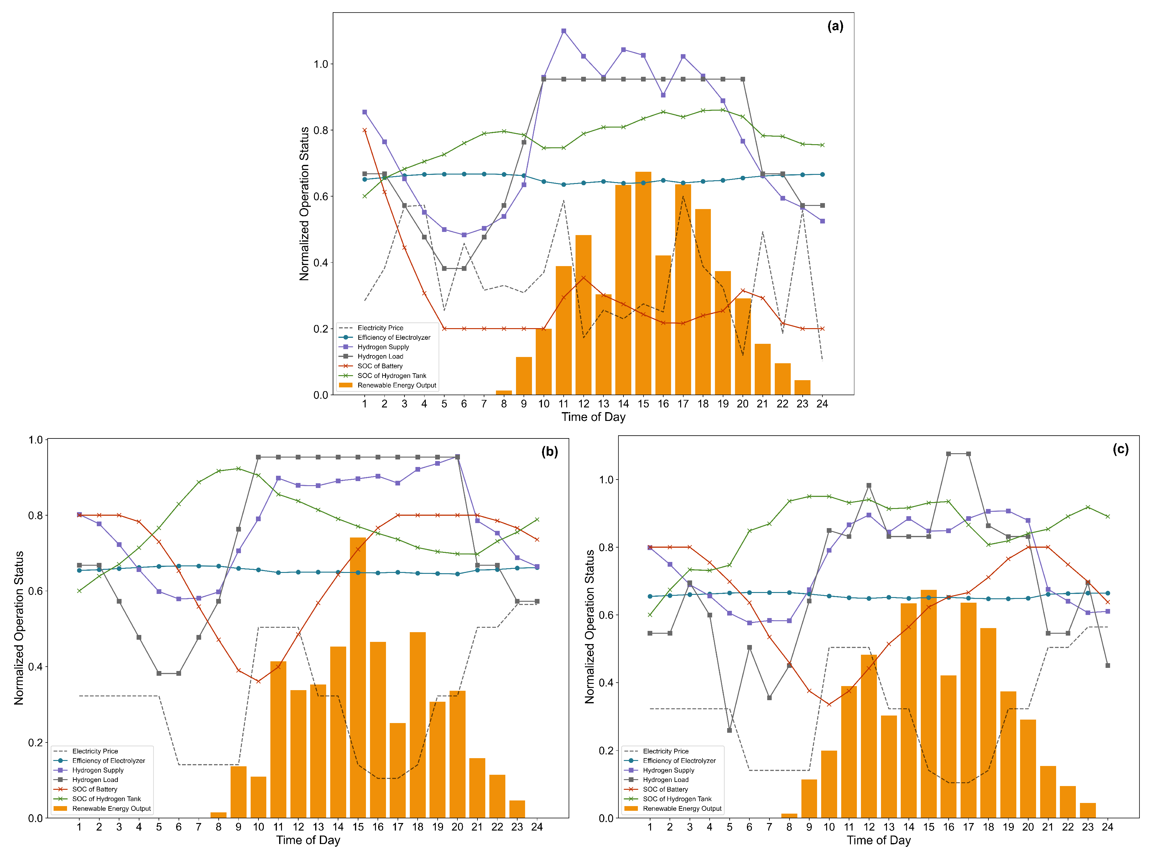
Analysis of Operational Strategies

In Scenario 1, the renewable energy output fluctuates significantly and peaks during the midday hours, accounting for 70% of the rated system capacity. This reflects the typical daytime pattern of solar power generation. Given the high cost of storing electricity over extended periods, the energy storage system employs nighttime low-through tariffs for discharging and recharges during periods of high renewable energy output and low tariffs to adapt to time-sharing tariffs. The hydrogen storage system performs electrolysis for hydrogen production during the nighttime low-tariff hours and elects to operate at higher power during these hours. This decision is made with the understanding that the low load at night may result in a decrease in the efficiency of the electrolyzer. Consequently, there is a minor loss of hydrogen in the morning from 7 to 8 a.m. (0.14 units). During the midday period of high load, the system employs a strategy of reducing power consumption and utilizing hydrogen from the hydrogen storage tanks to mitigate a decline in electrolyzer efficiency. The rationale behind the increase in hydrogen storage during nighttime hours remains consistent.

In Scenario 2, the hydrogen storage tank attains its maximum capacity one hour earlier due to the increased number of low-production hours at night during the winter months. However, the new energy output exhibits greater smoothness in the winter months, thereby enabling the system to more efficiently utilize the hydrogen storage tank to balance the electrolyzer efficiency and mitigate the challenge of a lack of sunlight. The incorporation of an additional hour during the evening’s high-production period marginally reduces the demand on the hydrogen storage tanks during nocturnal hours. In Scenario 3, the hydrogen storage tank’s capacity is diminished to 20 MW, leading to heightened hydrogen losses during morning hours. This is attributable to the constrained hydrogen storage during periods of minimal demand. Despite the high new energy output in the middle of the day, the average efficiency of the electrolyzer decreases slightly, indicating the need to find a new balance between efficiency and availability with limited storage. The smart body, therefore, focuses on energy storage devices to accumulate energy during the high output hours for use during the evening high tariff hours. In Scenario 4, the constant efficiency electrolyzer model (${\eta }_e=0.6$) reduces the regulation function of the hydrogen storage device, retaining only the effect of hydrogen production during the nighttime low-tariff hours. At this juncture, the functions of hydrogen storage and energy storage become intertwined. Due to the relatively long benefit transfer path of hydrogen storage, the intelligent body tends to prioritize the charging and discharging operation of the energy storage, and thus, may neglect the role of the hydrogen storage tank in regulating the operation of the electrolyzer. In this case, the electrolyzer may over-adapt to demand fluctuations during the day, which may reduce its operational efficiency during dramatic changes in demand.

In evaluating the alterations in electrolyzer efficiency, the ramifications of efficiency fluctuations on the expense of procured energy and operational and maintenance (O&M) expenditures have been previously taken into account, a practice that is pertinent for industrial production cost management. Nevertheless, the significance of energy conservation extends beyond mere economic considerations, being concomitantly associated with the enhancement of energy utilization efficiency. Consequently, we propose the incorporation of the average efficiency of the electrolyzer within the reward function, with the objective of incentivizing the pursuit of energy efficiency enhancement. In Scenario 5, this strategy results in a more even electrolyzer operating curve, particularly during the midday hours. The hydrogen storage tank assumes a more significant role in power balancing, preventing hydrogen wastage and leveraging the stored hydrogen to preserve the high efficiency of the electrolyzer during midday. By modifying the reward function, the intelligences can more readily identify efficient energy utilization strategies, enabling them to prioritize optimal battery usage. This entails discharging during morning hours when electricity prices are elevated and recharging during midday when prices are reduced, thereby maximizing battery efficiency.

A synthesis of the results of the analysis of the five scenarios reveals that the primary function of the energy storage device is to enhance the system’s adaptability to time-of-day tariffs, thereby reducing the cost of purchased electricity. The synergistic effect of the hydrogen storage tank and electrolyzer is twofold: first, they enhance the system’s adaptability to changes in electricity prices, and second, the output power of the electrolyzer directly affects its efficiency, which in turn affects the operating costs and energy utilization efficiency. Therefore, the hydrogen storage tank plays a key role in smoothing the output of the electrolyzer and maintaining its efficiency stability. The variable operating condition model of the electrolyzer and the capacity of the hydrogen storage tank collectively determine the degree of attention devoted by the intelligentsia to the efficiency stability of the electrolyzer. A comparative analysis of scenarios reveals that under high-capacity and variable-condition conditions, the intelligent bodies place greater emphasis on the benefits brought by the efficiency stability of the electrolyzer. Conversely, as the hydrogen storage tank capacity diminishes and the constant operating condition model is implemented, the intelligent body’s focus shifts to the alignment of the electrolyzer output with the demand curve and the regulatory function of energy storage within the system.

A thorough examination reveals that the initial production load scheduling strategy employed by the polysilicon plant is inadequate. The strategy’s limitations stem from its exclusive consideration of electricity price impacts on cost, while disregarding the variability in equipment efficiency under changing operating conditions. During periods of high new energy generation, the strategy’s excessive emphasis on production leads to a decline in electrolyzer efficiency. However, through the optimization of the scheduling strategy, a more rational production arrangement can be attained by leveraging the hydrogen storage device. The decline in production after 8:00 p.m., particularly during nighttime hours, is attributed to the escalating costs associated with electricity. However, this decline is also influenced by the capacity of the storage device and the inherent inefficiency and cost implications of the electrolyzer. To address these challenges, a balanced allocation of daytime and nighttime production is imperative. Specifically, there is a need to augment nighttime production to alleviate the strain on hydrogen storage tanks.

4.4. Cost Analysis

As demonstrated in

Table 3. Cost comparison of different scene.

Scenario	Power Purchase Cost	Emission Cost	Operation and Maintenance Cost	Total Cost	Reward Value
Basic Model	1,584,499.74	295,927.92	505,999.35	2,386,427.0	−22.03
Modified Reward Function	1,587,993.84	295,941.43	501,338.00	2,385,273.3	−21.84
Modified Hydrogen Storage Capacity	1,583,686.27	295,402.55	507,575.39	2,386,664.2	−26.42
Fixed Working Conditions	1,579,777.19	295,189.11	512,174.31	2,387,140.6	−32.75

, a cost analysis was conducted on the operation optimization results under the aforementioned scenarios. Scenario 1, serving as the baseline model, exhibited a total cost of 2,386,427. The power purchase cost, carbon emission cost, and O&M cost accounted for 66.45%, 12.43%, and 21.20%, respectively. The total costs for Scenarios 3 and 5 decreased by 0.032% and 0.040%, respectively, while the total costs for Scenario 4 increased by 0.027%. These findings indicate that adjusting the reward function and hydrogen storage capacity has a positive, albeit limited, impact on cost-effectiveness. Specifically, Scenario 2 achieves a reduction in total expenditures by adjusting the reward function, which slightly increases the cost of electricity but significantly reduces O&M costs. This strategy improves energy efficiency by upgrading the performance of the electrolyzer and contributes to more cost-effective operations. In Scenario 5, incorporating the average efficiency of the electrolyzer into the reward function achieves a further reduction in costs by precisely adjusting the relationship between power costs and O&M expenses, increasing the reward value to −21.84. In contrast, the constant load electrolyzer model, despite achieving a lower power purchase cost, results in an increase in O&M cost, leading to an overall rise in costs. This is attributable to the inability of the constant efficiency model to be dynamically adjusted according to real-time tariffs and load demand during operation. Conversely, the variable load electrolyzer model attains a more balanced cost distribution by adjusting its operation strategy with greater flexibility, thereby enhancing the overall economics, albeit with a slight increase in power purchase cost.

4.5. Sensitivity Assessment

This study proposes a sensitivity analysis, building upon the findings of five previous scenario analyses, with the objective of investigating the impact of key parameter fluctuations on the stability of the system operation optimization strategy. In consideration of the source-load uncertainty encountered by the polysilicon park energy supply system in actual operation, this study selects three key parameters for analysis: electricity price, renewable energy output, and load demand. The fluctuation of electricity price is directly related to the energy procurement cost, while the fluctuation of renewable energy output and load demand affects the energy balance and operation efficiency of the system. These parameters have a decisive impact on the determination of the optimal operation strategy of the energy system. Based on the analysis of environmental fluctuations on a typical summer dispatch day, the impact of key parameter changes on the robustness and effectiveness of system control is systematically evaluated, and the results are shown in

Table 4. Efficiency comparison under different scenarios.

Scenario	Hydrogen Unsatisfaction Rate	Efficiency Average Value	Efficiency Range	Efficiency Variance
Electricity Price Fluctuation	0	0.654	0.032	0.108
Renewable Output Fluctuation	0	0.655	0.021	0.007
Demand Fluctuation	0	0.657	0.018	0.007

.

Figure 9a illustrates that the system parameters undergo fluctuations due to the stochastic variations in electricity prices during a typical summer day. The control strategy employed by the system effectively caters to the fluctuating demand for hydrogen, while ensuring that the hydrogen unfulfillment rate remains zero and there is no hydrogen wastage. Furthermore, the system maintains the electrolyzer efficiency at a consistently high level through its interaction with the hydrogen storage tank, achieving an average efficiency of 0.654 and thereby achieving an energy-saving effect. The energy storage battery exhibits a certain degree of load smoothing functionality, capable of recognizing and mitigating the fluctuations in electricity prices, thereby reducing the cost of electricity acquisition through charging and discharging. However, its capacity is constrained, precluding the full utilization of the energy storage battery’s potential.

Figure 9b illustrates the impact of renewable energy output fluctuations on the robustness of system control. Given that renewable energy output typically exhibits clear cyclical characteristics, the application of random fluctuations with a fixed mean value in each time period is inadequate for accurately reflecting these fluctuations. Consequently, a fluctuation factor conforming to a standard normal distribution, derived from the raw output data, was introduced to more precisely evaluate the stability and adaptability of the system. The results demonstrate that the hydrogen load is adequately met, the mean efficiency is enhanced to 0.655, and the efficiency extreme deviation and variance are reduced to 0.021 and 0.007, respectively. It is noteworthy that the performance of the storage battery is considerably improved under the regression to the normal time-of-day tariff, indicating that the control strategy of the storage battery remains sensitive to the tariff.

Figure 9c illustrates the impact of demand fluctuations on the stability of the control system. The system incorporates a standard normally distributed disturbance term to the original hydrogen demand, thereby assessing the system’s resilience to short-term demand fluctuations. The results demonstrate that the system continues to meet the hydrogen load and the average value of the electrolyzer efficiency is enhanced to 0.657. The observed fluctuations in the state of the hydrogen storage tank underscore the significance of its integration with the electrolyzer in ensuring the stability of electrolyzer efficiency. In summary, the control strategy proposed in this study demonstrates notable adaptability and robustness in the face of fluctuations in electricity prices, renewable energy output, and demand. It effectively meets the load demands of the production process while ensuring the efficient operation of electrolyzer equipment, thereby achieving the objective of energy savings and efficiency.

4.6. Comprehensive Benefits Analysis of Low-Carbon Transformation

This section is based on an in-depth analysis of the low-carbon economic operation optimization model of the polysilicon park’s energy supply system and its operation strategy. The objective of this analysis is to further evaluate the carbon emission reduction effect and economic performance achieved by the system in actual engineering applications. Through quantitative analysis, it was determined that under the original direct purchased power scenario, the daily carbon emission obtained by using the 2022 national average CO₂ emission factor for electricity is 3,488,147 kg. In contrast, with the system and its operation strategy proposed in this study, the daily carbon emission of the plant is reduced to 2,465,889 kg [28], achieving a carbon reduction effect of 29.3%. In terms of the single-day operating cost, the original system operating cost was 2,173,042, while the minimum operating cost of the system under consideration was 2,385,273 (Scenario 5).

A more thorough examination of the carbon emission composition of the system illuminates that PV equipment continues to account for a significant portion of carbon emissions, primarily due to its lower power density and higher production-related carbon emissions. This outcome underscores the imperative for mitigating the production carbon emissions of the entire PV equipment industrial chain to facilitate the decarbonization of power systems and industrial production. This underscores the significance of this study in the industrial and energy sectors.

While the energy storage battery and hydrogen storage tank enhance the system’s flexibility in meeting time-of-use tariffs and the stability of electrolyzer efficiency, the high operational cost of renewable energy devices, particularly solar cells, renders the system less economical than direct power purchase. This underscores the challenges faced by the renewable energy equipment manufacturing industry in reducing costs.

With respect to the electrolyzer’s energy utilization efficiency, the original system exhibits an average efficiency of 0.620, attributable to demand fluctuations. However, under the control strategy of this system, the average efficiency increases to 0.655 through the integration of the electrolyzer with the hydrogen storage tank equipment. This enhancement in efficiency facilitates the production of more hydrogen with reduced energy expenditure, thereby signifying a substantial improvement in energy utilization. It is evident that the existing system can effectively reduce the electrolyzer operation cost, as the levelized energy operation cost is directly proportional to the energy utilization efficiency.

In summary, the new energy transformation of the power supply side has the potential to significantly reduce the carbon emissions of the polysilicon reduction process, thereby further reducing power carbon emissions and creating a positive cycle. However, this transformation can also result in increased costs for enterprises and production costs; they can use hydrogen supply side equipment coupling and the reinforcement learning algorithm control to achieve the unity of energy utilization and production economy, while electrolyzer control can realize the equipment layer, data layer, algorithm layer separation, with its transformation difficulty being low. Consequently, enterprises stand to benefit significantly from the transformation of electrolyzer–hydrogen storage tank equipment. However, the comprehensive implementation of new energy–hydrogen production and storage methods remains contingent on the cost reduction and efficiency enhancement of upstream and downstream industries.

4.7. Different Algorithm Contrast

This section provides insights into the effectiveness of three deep reinforcement learning algorithms—TD3, DDPG, and DQN—applied to the dynamic scheduling problem of integrated energy systems and compares the operating cost, emission cost, as well as total cost of these algorithms over a typical day. As shown in

Table 5. Cost comparison of different algorithms.

Algorithm	Emission Cost	Operation Cost	Total Cost	Reward Value
TD3	295,927.92	501,338	797,265.92	−22.03
DDPG	307,173.18	504,362.15	811,535.33	−28.08
DQN	321,377.72	507,153.67	828,531.39	−43.12
CPLEX	291,489.00	500,221.39	791,710.39	-

, the TD3 algorithm demonstrates a significant advantage in terms of overall cost-effectiveness, with a reduction in average daily operating cost of about 0.6% and 1.2%, and a reduction in emission cost of about 2.0% and 12.0%, respectively, compared to the DDPG and DQN algorithms. These results indicate that the TD3 algorithm provides a more economical and environmentally friendly solution. Further comparing the TD3 and CPLEX algorithms, we find that the average daily operating cost of TD3 is comparable to that of CPLEX. This confirms the usefulness of the TD3 algorithm in dealing with real-time optimal scheduling problems in integrated energy systems. Although CPLEX is more accurate in static optimization problems, the adaptability and real-time nature of the TD3 algorithm makes it perform better in dynamic environments. The TD3 algorithm shows high efficiency and stability in the new energy–hydrogen production, storage, and utilization system in the polysilicon park. However, the model convergence path analysis shows that the TD3 algorithm suffers from multi-hyperparameter sensitivity problems, which may cause training and tuning challenges in practical applications. In particular, it is difficult to balance exploration and exploitation when the action space is complex. In addition, although the TD3 algorithm uses dual Q-networks to improve learning stability, this can also lead to an increase in computational cost, which is a potential barrier in industrial applications.

5. Conclusions

In this study, a low-carbon economic dispatch strategy based on the TD3 algorithm is proposed and validated for a renewable hydrogen production and storage system in the polysilicon park, with the following main contributions:

• Equipment coupling and efficiency improvement: in this study, a dynamic physical model of electrolyzer with variable operating conditions is constructed and combined with the XGBoost agent model, which effectively improves the flexibility of system operation and energy utilization efficiency. The results of the study show that the total system cost decreases by about 0.027% after the introduction of the variable operating condition model. The energy storage device effectively reduces the cost of purchased electricity and improves the adaptability of the system to fluctuations in electricity prices. The synergy between the hydrogen storage device and the electrolyzer significantly improves the energy utilization efficiency, and the hydrogen storage device maintains the stability of its efficiency by smoothing the electrolyzer output.
• Performance advantages and disadvantages of the TD3 algorithm: the TD3 algorithm shows high efficiency and stability in this system. Compared with the DDPG and DQN algorithms, the TD3 algorithm reduces the average daily operation cost by about 0.6% and 1.2%, and the carbon emission cost by about 2.0% and 12.0%, respectively. Through the comparative analysis of five different operation scenarios and three environmental fluctuation cases, the adaptability of the TD3 algorithm in different environments and operation conditions is verified, showing strong robustness and generalization ability. However, at the same time, the convergence path of the model shows that it has problems such as many hyperparameters and hyperparameter sensitivity, which brings certain obstacles to the tuning in practical application.
• Evaluation of the low-carbon economy effect: the new energy transformation on the power supply side significantly reduces the carbon emission of the polysilicon reduction process, achieving a carbon reduction effect of 29.3%, but the high operating cost of renewable energy devices, especially solar cells, still makes the system less economical than direct power purchase. Optimizing the operation of the coupled part of electrolyzer and hydrogen storage tank is the most likely part of the system to achieve industrial applications, considering various dimensions, such as economy, energy saving and efficiency improvement, and equipment modification.

To address the above issues, future research will continue to optimize the hyperparameters of the TD3 algorithm, reduce the computational cost, and explore more efficient renewable energy devices to improve the system economy. Meanwhile, the coupling mechanism between hydrogen storage tank and electrolyzer will be studied in depth to improve the adaptability and stability of the system. Specific directions include: adaptive hyperparameter tuning, enhancing the exploration capability of TD3, and exploring the combination of cluster control strategy and deep reinforcement learning. In addition, it is planned to optimize the network structure of the algorithm to account for the influence of the carbon capture device, and to verify it through practical engineering, in order to improve the learning ability of the intelligences and provide more powerful support for intelligent optimal scheduling of the energy system.

References

1. Wang, Y.; Zhao, X.; Huang, Y. Low-Carbon-Oriented Capacity Optimization Method for Electric–Thermal Integrated Energy System Considering Construction Time Sequence and Uncertainty. Processes 2024, 12, 648. [Google Scholar] [CrossRef]
2. Yang, J.; Xie, L.; Song, X.; Ye, H.; Zhang, P.; Bian, Y. Optimal Configuration of PV-Fire-Hydrogen Polysilicon 787 Park Based on Multivariate Copula Function. Acta Energiae Solaris Sinica. Acta Energiae Solaris Sin. 2023, 44, 180–188. [Google Scholar] [CrossRef]
3. Ramírez-Márquez, C.; Martín-Hernández, E.; Martín, M.; Segovia-Hernández, J.G. Surrogate based optimization of a process of polycrystalline silicon production. Comput. Chem. Eng. 2020, 140, 106870. [Google Scholar] [CrossRef]
4. Saravanan, S.; Mahadevan, M.; Suratkar, P.; Gijo, E.V. Efficiency improvement on the multicrystalline silicon wafer through six sigma methodology. Int. J. Sustain. Energy 2012, 31, 143–153. [Google Scholar] [CrossRef]
5. Mohammed, A.; Ghaithan, A.M.; Al-Hanbali, A.; Attia, A.M. A multi-objective optimization model based on mixed integer linear programming for sizing a hybrid PV-hydrogen storage system. Int. J. Hydrogen Energy 2023, 48, 9748–9761. [Google Scholar] [CrossRef]
6. Ruiming, F. Multi-objective optimized operation of integrated energy system with hydrogen storage. Int. J. Hydrogen Energy 2019, 44, 29409–29417. [Google Scholar] [CrossRef]
7. Hong, Z.; Wei, Z.; Han, X. Optimization scheduling control strategy of wind-hydrogen system considering hydrogen production efficiency. J. Energy Storage 2022, 47, 103609. [Google Scholar] [CrossRef]
8. Kafetzis, A.; Ziogou, C.; Panopoulos, K.; Papadopoulou, S.; Seferlis, P.; Voutetakis, S. Energy management strategies based on hybrid automata for islanded microgrids with renewable sources, batteries and hydrogen. Renew. Sustain. Energy Rev. 2020, 134, 110118. [Google Scholar] [CrossRef]
9. Pu, Y.; Li, Q.; Zou, X.; Li, R.; Li, L.; Chen, W.; Liu, H. Optimal sizing for an integrated energy system considering degradation and seasonal hydrogen storage. Appl. Energy 2021, 302, 117542. [Google Scholar] [CrossRef]
10. Zhang, L.; Wu, H.; He, Y.; Xu, B.; Zhang, M.; Ding, M. Optimal Scheduling Method for Integrated Energy Systems with Hydrogen Based on Deep Reinforcement Learning. Autom. Electr. Power Syst. 2024, 48, 132–141. [Google Scholar] [CrossRef]
11. Perera, A.; Kamalaruban, P. Applications of reinforcement learning in energy systems. Renew. Sustain. Energy Rev. 2021, 137, 110618. [Google Scholar] [CrossRef]
12. Shi, T.; Xu, C.; Dong, W.; Zhou, H.; Bokhari, A.; Klemeš, J.J.; Han, N. Research on energy management of hydrogen electric coupling system based on deep reinforcement learning. Energy 2023, 282, 128174. [Google Scholar] [CrossRef]
13. Zhang, Z.; Qiu, C.; Zhang, D.; Xu, S.; He, X. A Coordinated Control Method for Hybrid Energy Storage System in Microgrid Based on Deep Reinforcement Learning. Power Syst. Technol. 2019, 43, 1914–1921. [Google Scholar] [CrossRef]
14. Liu, J.; Chen, J.; Wang, X.; Zeng, J.; Huang, Q. Energy Management and Optimization of Multi-Energy Grid Based on Deep Reinforcement Learning. Power Syst. Technol. 2020, 44, 3794–3803. [Google Scholar] [CrossRef]
15. Huang, W.; Li, Q.; Jiang, Y.; Lu, X. Parametric Dueling DQN- and DDPG-Based Approach for Optimal Operation of Microgrids. Processes 2024, 12, 1822. [Google Scholar] [CrossRef]
16. Xu, B.; Xiang, Y. Optimal operation of regional integrated energy system based on multi-agent deep deterministic policy gradient algorithm. Energy Rep. 2022, 8, 932–939. [Google Scholar] [CrossRef]
17. Fujimoto, S.; van Hoof, H.; Meger, D. Addressing Function Approximation Error in Actor-Critic Methods. In Proceedings of the International Conference on Machine Learning, Stockholm, Sweden, 10–15 July 2018. [Google Scholar]
18. Hou, S.; Salazar, E.M.; Vergara, P.P.; Palensky, P. Performance Comparison of Deep RL Algorithms for Energy Systems Optimal Scheduling. In Proceedings of the 2022 IEEE PES Innovative Smart Grid Technologies Conference Europe (ISGT-Europe), Novi Sad, Serbia, 10–12 October 2022; pp. 1–6. [Google Scholar] [CrossRef]
19. Deng, J.; Jiang, F.; Wang, W.; He, G.; Zhang, X.; Liu, K. Low-carbon Optimized Operation of Integrated Energy System Considering Electric-Heat Flexible Load and Hydrogen Energy Refined Modeling. Power Syst. Technol. 2022, 46, 1692–1704. [Google Scholar] [CrossRef]
20. Zhang, X.; Peng, H.; Cao, F.; Cao, Y.; Liu, Q.; Tang, C.; Zhou, T. Study on the influence characteristics of multi-working condition parameters on membrane electrode type CO2 electrolyzer. Int. J. Electrochem. Sci. 2024, 19, 100870. [Google Scholar] [CrossRef]
21. Ma, B.; Zheng, J.; Xian, Z.; Wang, B.; Ma, H. Optimal Operation Strategy for Wind–Photovoltaic Power-Based Hydrogen Production Systems Considering Electrolyzer Start-Up Characteristics. Processes 2024, 12, 1756. [Google Scholar] [CrossRef]
22. Klyuev, R.; Madaeva, M.; Umarova, M. Mathematical Modeling of Specific Power Consumption of Electrolyzers. In Proceedings of the 2020 International Ural Conference on Electrical Power Engineering (UralCon), Chelyabinsk, Russia, 22–24 September 2020; pp. 356–361. [Google Scholar] [CrossRef]
23. Wei, X.; Sharma, S.; Waeber, A.; Wen, D.; Sampathkumar, S.N.; Margni, M.; Maréchal, F.; Van Herle, J. Comparative life cycle analysis of electrolyzer technologies for hydrogen production: Manufacturing and operations. Joule 2024, 8, 3347–3372. [Google Scholar] [CrossRef]
24. Scheepers, F.; Stähler, M.; Stähler, A.; Rauls, E.; Müller, M.; Carmo, M.; Lehnert, W. Improving the Efficiency of PEM Electrolyzers through Membrane-Specific Pressure Optimization. Energies 2020, 13, 612. [Google Scholar] [CrossRef]
25. Scheepers, F.; Stähler, M.; Stähler, A.; Rauls, E.; Müller, M.; Carmo, M.; Lehnert, W. Temperature optimization for improving polymer electrolyte membrane-water electrolysis system efficiency. Appl. Energy 2021, 283, 116270. [Google Scholar] [CrossRef]
26. Durisch, W.; Bitnar, B.; Mayor, J.C.; Kiess, H.; Lam, K.h.; Close, J. Efficiency model for photovoltaic modules and demonstration of its application to energy yield estimation. Sol. Energy Mater. Sol. Cells 2007, 91, 79–84. [Google Scholar] [CrossRef]
27. Emrani, A.; Achour, Y.; Sanjari, M.J.; Berrada, A. Adaptive energy management strategy for optimal integration of wind/PV system with hybrid gravity/battery energy storage using forecast models. J. Energy Storage 2024, 96, 112613. [Google Scholar] [CrossRef]
28. Elaouzy, Y.; El Fadar, A.; Achkari, O. Assessing the 3E performance of multiple energy supply scenarios based on photovoltaic, wind turbine, battery and hydrogen systems. J. Energy Storage 2024, 99, 113378. [Google Scholar] [CrossRef]
Figure 1. Electrolyzer efficiency characteristic curve.
Processes 13 00268 g001
Figure 2. Surrogate model prediction curve.
Processes 13 00268 g002
Figure 3. Energy system architecture.
Processes 13 00268 g003
Figure 4. TD3 algorithm network architecture.
Processes 13 00268 g004
Figure 5. Weather prediction based on VMD-CNN-BiLSTM-Attention.
Processes 13 00268 g005
Figure 6. Normalized data of irradiation, wind speed, load, and electricity price.
Processes 13 00268 g006
Figure 7. Convergence curves of the TD3 algorithm under different hyperparameters.
Processes 13 00268 g007
Figure 8. Dispatching strategy in different condition (a) energy balance in scenario 1; (b) typical summer condition; (c) typical winter condition; (d) reduced hydrogen tank capacity; (e) constant electrolyzer efficiency; (f) introducing average electrolyzer efficiency.
Processes 13 00268 g008
Figure 9. Sensitivity analysis under price, renewable energy, and hydrogen demand volatility (a) price volatility; (b) renewable energy volatility; (c) hydrogen demand volatility.
Processes 13 00268 g009