Two-Layer Optimal Scheduling Model of Microgrid Considering Demand Response Based on Improved Nutcracker Optimization Algorithm

Abstract

To comprehensively address the interests of both the supply and demand sides within a microgrid, a two-layer optimal scheduling model incorporating demand response was formulated. The upper tier aims to optimize the load profile, focusing on maximizing electricity consumption satisfaction and minimizing user electricity costs. Meanwhile, the lower tier targets the optimization of output from each controllable generation unit, with the goal of reducing operational costs. Given the nonlinear and multi-constrained nature of this model, an improved nutcracker optimization algorithm (INOA) is proposed. This enhancement introduces chaotic sequences into the original nutcracker optimization algorithm (NOA) for population initialization, employs a hybrid butterfly optimization algorithm to enhance the algorithm’s local search capabilities, and integrates dynamic selection adaptive T-distribution for updating individual positions. The solution tests involving INOA, NOA, dung beetle optimizer (DOB), particle swarm optimization (PSO), grey wolf optimization (GWO), and sparrow search algorithm (SSA) were conducted using the CEC2022 intelligent algorithm test suite. Analysis reveals that INOA exhibits superior comprehensive optimization performance compared to other algorithms, validating the effectiveness of the improvements introduced in this paper. Ultimately, a simulation analysis of the microgrid was performed, demonstrating that, despite a 3.58% reduction in user satisfaction, participation in demand response led to a 25.16% decrease in electricity costs and a 5.92% reduction in microgrid operational costs. These findings substantiate the model’s capability to effectively balance the economic interests of both the supply and demand sides within the microgrid.

1. Introduction

In recent years, the rapid advancement of the economy has significantly improved people’s quality of life, while it has also led to an increasing demand for power energy. The rapid consumption of fossil fuels has exacerbated global energy depletion. To address these challenges, the development of diversified microgrid structures has gained attention as a means to alleviate the depletion of traditional fossil fuels and mitigate environmental issues. Consequently, research on optimal scheduling based on microgrid modeling and scheduling strategies has attracted widespread interest [1,2]. At present, microgrid dispatch must consider both the generation side and the demand side’s participation in load adjustment [3,4]. He et al. [5] introduced real-time pricing (RTP) based on time-of-use electricity prices and implemented a demand response plan according to RTP. Zhang et al. [6] proposed a multi-objective scheduling model to maximize the profits of power companies and demand users, optimizing the time-of-use electricity price using the linear function of load demand elasticity. The practicality of this multi-objective scheduling model was verified through five test cases. Rana et al. [7] proposed a distributed collaborative operation optimization method for multilateral participants, achieving collaborative operation guided by dynamic time-of-use electricity prices. Internationally and domestically, research on microgrid dispatch primarily focuses on single-objective economic dispatch. Phommixay, S. et al. [8] optimized the dispatch of distributed energy sources through a two-stage dispatch to minimize the operational costs of the microgrid. Dawei Zhao et al. [9] developed real-time economic scheduling algorithms to enhance the operation of microgrids, especially those involving wind, diesel, and energy storage systems. Li et al. [10] developed a multi-objective hierarchical microgrid economic dispatch strategy for load levels, source-load levels, and source-grid-load levels based on the operational characteristics of each dispatch unit. Hwang Goh, H. et al. [11] treated economic dispatch as a discrete optimal control problem and constructed a microgrid economic optimization dispatch model based on dynamic programming.

However, these studies have not adequately considered the absorption of excess renewable energy output by the load or the balance of the microgrid through the addition of energy storage systems when optimizing load management. Future research should focus on effectively integrating energy storage systems to promote the rational allocation and utilization of resources within the microgrid, thereby enhancing its overall economic efficiency and environmental benefits.

Microgrid optimization scheduling presents a multifaceted challenge characterized by numerous dimensions and constraints, necessitating the application of sophisticated intelligent algorithms for effective solutions. Among the prominent techniques in this domain are particle swarm optimization (PSO), the sparrow search algorithm (SSA), genetic algorithms (GA), and so on. However, these algorithms, in their original forms, exhibit certain limitations that have driven researchers to refine existing methods [12,13] or investigate novel algorithms for enhanced optimization capabilities [14,15]. For instance, Wang et al. [16] demonstrated the successful application of an enhanced multi-objective grey wolf optimizer (MO-GWO) to the complex task of optimizing a combined cooling, heating, and power (CCHP) microgrid model. This approach showcases outstanding global exploration efficiency and accelerated computational dynamics. Meanwhile, Dong et al. [17] introduced an innovative variant of PSO that employs a quadratic sequence strategy to expand the search space, specifically designed to address intricate planning challenges. Jian Fang et al. [18], by combining the powerful optimization capabilities of genetic algorithm (GA) with PSO, adopted an improved PSO-GA algorithm to solve the optimization scheduling model of offshore wind power microgrids, achieving a reduction in carbon emissions while ensuring the optimal economic performance of the system. Despite these advancements, the literature lacks comprehensive cross-comparisons between these advanced algorithms and other cutting-edge intelligent algorithms, thus failing to fully substantiate their absolute performance advantages.

In light of demand response considerations, the present paper proposes a two-layer optimization model for microgrids [19]. The upper layer focuses on enhancing user satisfaction and minimizing user costs, while the lower layer targets the reduction in microgrid operational costs. To address the issue of slow convergence in the nutcracker optimization algorithm (NOA), an improved nutcracker optimization algorithm (INOA) is introduced. The effectiveness of INOA is validated through comparative analysis of its iterative results against those of other algorithms via test functions.

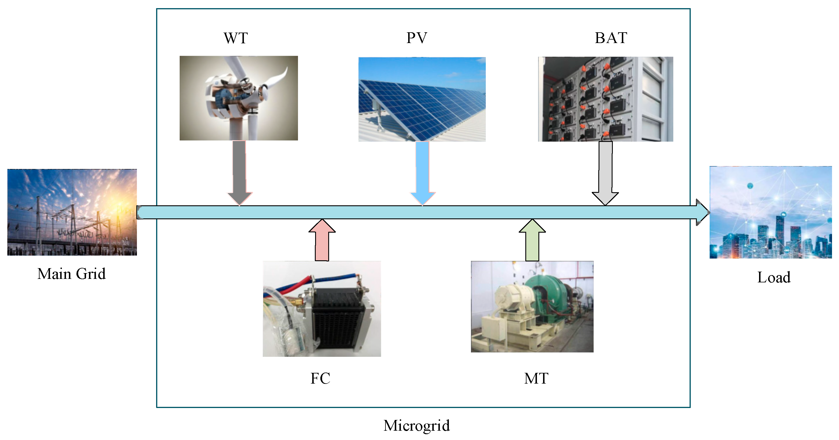
2. Microgrid Architecture

A microgrid can be defined as a compact system for power generation, distribution, and consumption, integrating both supply and demand components. This paper primarily focuses on the analysis of grid-connected microgrids that incorporate wind turbines (WT), photovoltaic systems (PV), fuel cells (FC), microturbines (MT), batteries (BAT), and demand-side loads. The architecture of the microgrid under consideration is illustrated in Figure 1, which provides a visual representation of the interconnected framework that serves as the foundation of this study.

This architecture ensures a balanced and efficient operation by leveraging the diverse strengths of each component. Wind turbines and photovoltaic systems supply renewable energy, while fuel cells and microturbines provide stable and reliable power generation. Batteries act as energy storage units, enabling the microgrid to handle fluctuations in supply and demand. The integration of demand-side loads facilitates dynamic load management, enhancing the overall flexibility and resilience of the microgrid. Collectively, these elements form a robust and sustainable power system capable of meeting the varied energy needs of the connected users.

3. Price-Based Demand Response Model Based on User Compensation

3.1. Demand Response Model

Price-driven demand response (PDR), as discussed in references [7,20], fundamentally operates by utilizing time-of-use (TOU) pricing mechanisms as key signals to adjust and guide consumer energy consumption patterns. However, this approach has shown limitations in effectively motivating active user participation. To address this issue, our work introduces an innovative strategy that integrates TOU pricing mechanisms with incentivized compensation schemes. This dual-faceted approach is designed to optimize consumer electricity usage patterns and structures, reducing peak-hour consumption, increasing off-peak energy use, and ultimately lowering electricity expenses for end-users.

Current research in this field largely relies on electricity-price elasticity matrices as a tool to quantify consumer responsiveness to tariff changes. These matrices serve as the foundation for constructing models that capture user behavior under different price signals. The mathematical expression for this relationship is represented as follows:

$${\epsilon }_{kt}={\displaystyle \frac{∆P_L\left(k\right)/P_L^0\left(k\right)}{∆D\left(t\right)/D^0\left(t\right)}}$$

(1)

In this equation, ${\epsilon }_{kt}$ represents the electricity price elasticity coefficient [21], which indicates the degree to which the user’s load changes at time k respond to the price changes at time t. When $k=t$, it is the self-elasticity coefficient, and when $k\ne t$, it is the inter-elasticity coefficient. In this paper, the scheduling time is 24 h, so the electricity price elasticity matrix is as follows:

$$\epsilon =\left[\begin{array}{ccc}\begin{array}{cc}{\epsilon }_{11}& {\epsilon }_{12}\\ {\epsilon }_{21}& {\epsilon }_{22}\end{array}& \cdots & \begin{array}{c}{\epsilon }_{1 24}\\ {\epsilon }_{2 24}\end{array}\\ ⋮& \ddots & ⋮\\ \begin{array}{cc}{\epsilon }_{24 1}& {\epsilon }_{24 2}\end{array}& \cdots & {\epsilon }_{24 24}\end{array}\right]$$

(2)

The amount of customer load change after customer participation in PDR is as follows:

$$\left[\begin{array}{c}∆P_L\left(1\right)/P_L^0\left(1\right)\\ ∆P_L\left(2\right)/P_L^0\left(2\right)\\ \cdots \\ ∆P_L\left(24\right)/P_L^0\left(24\right)\end{array}\right]=\epsilon ·\left[\begin{array}{c}∆D\left(1\right)/D^0\left(1\right)\\ ∆D\left(2\right)/D^0\left(2\right)\\ \begin{array}{c}\cdots \\ ∆D\left(24\right)/D^0\left(24\right)\end{array}\end{array}\right]$$

(3)

In this paper, the PDR model is constructed on the basis of minimizing the cost of electricity consumption by the user, so based on the initial electricity consumption of the user as well as the electricity consumption after the change of time-share tariffs, data such as the elasticity coefficient and the time-share tariffs are utilized to arrive at the final result:

$$P_{La}\left(t\right)=P_L\left(t\right)·({\epsilon }_{tt}·{\displaystyle \frac{∆D\left(t\right)}{D^0\left(t\right)}}+\sum _{\begin{array}{c}k=1\\ k\ne t\end{array}}^{24}{\epsilon }_{kt}·{\displaystyle \frac{∆D\left(k\right)}{D^0\left(k\right)}}+1)$$

(4)

where ${\epsilon }_{tt}$ is the self-elasticity coefficient; ${\epsilon }_{kt}$ is the mutual elasticity coefficient; $∆D\left(t\right)$ and $∆D\left(k\right)$ are the changes in the electricity price at moments t and k, respectively; $D^0\left(t\right)$ is the original electricity price before the user participates in the response; $P_L\left(t\right)$ is the load that participates in the PDR before the previous day; and $P_{La}\left(t\right)$ is the intra-day response dispatching electricity load of the user after participating in the PDR.

The compensation cost received by the customer participating in PDR is as follows:

$$W=\sum _{t=1}^T{((P}_L(t)-P_{La}\left(t\right))·C^{down}+{(P}_{La}(t)-P_L\left(t\right))·C^{up})·∆T$$

(5)

where $P_L\left(t\right)-P_{La}\left(t\right)$ denotes the downward electricity consumption of the user participating in PDR dispatch at moment t; $P_{La}\left(t\right)-P_L\left(t\right)$ denotes the upward electricity consumption of the user participating in PDR dispatch at moment t; and $C^{down}$ and $C^{up}$ denote the incentive prices for downward and upward adjustments during the day.

3.2. Demand Response Model Constraints

$$\sum _{t=1}^{24}{P}_{La}\left(t\right)·D\left(t\right)<\sum _{t=1}^{24}{P}_L\left(t\right)·D^0\left(t\right)$$

(6)

$$\sum _{t=1}^T{P}_{La}\left(t\right)=\sum _{t=1}^T{P}_L\left(t\right)$$

(7)

where $D^0\left(t\right)$ is the price of electricity at moment t before participation in demand response; $D\left(t\right)$ is the price of electricity at moment t after participation in demand response.

4. Bilevel Optimal Scheduling Model for Microgrids

To better utilize new energy generation and reduce wind and solar abandonment, this paper involves users in the optimal scheduling of the microgrid. A two-layer optimization model of the microgrid is established, taking into account user-side demand response. The upper layer focuses on minimizing the user’s power purchase cost and maximizing user satisfaction, optimizing the load profile through a demand response model. The lower layer represents the microgrid scheduling phase, aiming to minimize operational and environmental costs and is solved using the INOA.

4.1. Upper Optimization Model

To promote the consumption of new energy and reduce users’ power purchase costs, new load profiles are generated through peak shaving and valley filling based on the demand response model. Additionally, to minimize the impact of load shifting on users’ normal power consumption, user satisfaction is incorporated [22]. The upper-layer optimization objective function is formulated as follows [23]:

$$minC=0.7\left(\left(\sum _{t=1}^{T}D\left(t\right)\times P_{La}\left(t\right)\right)-W\right)+0.3\left(1-{\displaystyle \raisebox{1ex}{$\left(\frac{\sum _{t=1}^T\left|P_{La}\left(t\right)-P_L\left(t\right)\right|}{2}\right)$}\!\left/ \!\raisebox{-1ex}{$\sum _{t=1}^T{P}_L\left(t\right)$}\right.}\right)$$

(8)

In the formula, the first term represents the cost of electricity purchase, incorporating the TOU price, while the second term represents user satisfaction. Since the two functions have different dimensions, and this article focuses on optimization scheduling, it simplifies the impact of other factors, which does not consider the uncertainty and fluctuation of renewable energy, and uses a fixed-weight method to combine them into a single objective function. Here, T denotes the number of periods.

There are upper and lower limits for the transferable load, so the following constraints are added:

$$\left(1-\mu \right)P_L\left(t\right)\le P_{La}\left(t\right)\le \left(1+\mu \right)P_L\left(t\right)$$

(9)

where μ is the percentage of transferable load.

4.2. Lower Optimization Model

Under the load profile optimized by the upper layer, the lower layer objective function includes the fuel cost of the micro gas turbine $C_{MT}\left(t\right)$, the fuel cost of the fuel cell $C_{FC}\left(t\right)$, the operation and maintenance cost $C_{OM}\left(t\right)$, the cost of electricity transactions between the microgrid and the main grid $C_{grid}\left(t\right)$, and the start–stop cost of the micro gas turbine and fuel cell $C_{ST}\left(t\right)$ at time t. To maximize the economic benefits of the microgrid, the objective function is formulated to minimize the total operating cost, as shown in Equation (10):

$$min{C}_1=\sum _{t=1}^T\left(C_{MT}\left(t\right)+C_{FC}\left(t\right)+C_{OM}\left(t\right)+C_{ST}\left(t\right)+C_{grid}\left(t\right)\right)$$

(10)

and

$$C_{MT}\left(t\right)=C_{nl}{\displaystyle \frac{1}{LHV}}\sum {\displaystyle \frac{P_{MT}\left(t\right)}{{\eta }_{MT}\left(t\right)}}$$

(11)

$$C_{FC}\left(t\right)=C_{nl}{\displaystyle \frac{1}{LHV}}\sum {\displaystyle \frac{P_{FC}\left(t\right)}{{\eta }_{FC}\left(t\right)}}$$

(12)

$$C_{OM}\left(t\right)=C_{MT}\times P_{MT}\left(t\right)+C_{FC}\times P_{FC}\left(t\right)+C_{PV}\times P_{PV}\left(t\right)+C_{WT}\times P_{WT}\left(t\right)+C_{EB}\times P_{EB}\left(t\right)$$

(13)

$$C_{ST}\left(t\right)=C_{STMT}\times U_{MT}\left(t\right)+C_{STFC}\times U_{FC}\left(t\right)$$

(14)

$$C_{grid}\left(t\right)=C_{rb}\left(t\right)\times P_X\left(t\right)$$

(15)

where $C_{nl}$ is the local natural gas price (yuan/m³), i.e., 2.5 yuan/m³; LHV is the low calorific value of natural gas (kWh/m³), i.e., 9.7 kWh/m³; $P_{MT}\left(t\right)$ is the output power of the micro gas turbine at the moment t (kW); ${\eta }_{MT}\left(t\right)$ is the efficiency of the micro gas turbine at the moment t; $P_{FC}\left(t\right)$ is the output power of fuel cell at the moment t (kW); ${\eta }_{FC}\left(t\right)$ is the efficiency of fuel cell at the moment t; $C_{MT}, C_{FC}, C_{PV}, C_{WT}, \mathrm{a}\mathrm{n}\mathrm{d} C_{EB}$ are the operating costs (yuan/kW) of micro gas turbine, fuel cell, PV, wind, and storage battery; $C_{STMT}$ is the cost of gas turbine start and stop; $U_{MT}\left(t\right)$ (t) is whether or not the gas turbine is started at moment t; $C_{STFC}$ is the cost of fuel cell start and stop; $U_{FC}\left(t\right)$ is whether or not the fuel cell is starts; $C_{rb}\left(t\right)$ is the grid interaction tariff at moment t; and $P_X\left(t\right)$ is the power of grid interaction at moment t.

To ensure electric power balance at every moment in the microgrid, the following constraints must be satisfied:

$$P_{MT}\left(t\right)+P_{FC}\left(t\right)+P_{WT}\left(t\right)+P_{PV}\left(t\right)+P_X\left(t\right)+P_{EB}\left(t\right)/{\epsilon }_{eb}=P_{La}\left(t\right)$$

(16)

where ${\epsilon }_{eb}$ is the storage battery charging and discharging efficiency; $P_{EB}\left(t\right)$ is the power of the storage battery, which is positive for discharging and negative for charging.

Meanwhile, the battery energy storage initial and final states are equal constraints:

$$SOC\left(t\right)=SOC\left(t-1\right)-∆SOC$$

(17)

$$∆SOC=\left\{\begin{array}{c} {\displaystyle \frac{P_{EB}\left(t\right)∆t}{{\epsilon }_{eb}·E}} { P}_{EB}\left(t\right)\ge 0 \\ {\displaystyle \frac{P_{EB}\left(t\right)∆t·{\epsilon }_{eb}}{E}} P_{EB}\left(t\right)<0 \end{array}\right.$$

in Equation (17), $SOC\left(t\right)$ is the battery charge state at time t, $∆SOC$ is the change in charge state, and E is the battery capacity.

In order to ensure the safe and stable operation of the system, the output power of each controllable power generation unit is limited, and there exists an inequality constraint with the following constraint condition:

$${P_{n min}\le P}_n\left(t\right)\le P_{n max}$$

(18)

where $P_n\left(t\right)$ is the output power of the nth generation unit at moment t, and $P_{n min} \mathrm{a}\mathrm{n}\mathrm{d} P_{n max}$ are its upper and lower limits.

For gas turbine and fuel cell climbing, the constraints are as follows:

$$P_{MT}\left(t\right)-P_{MT}\left(t-1\right)\le r·∆t$$

(19)

$$P_{FC}\left(t\right)-P_{FC}\left(t-1\right)\le r·∆t$$

(20)

5. Improved Nutcracker Optimization Algorithm

5.1. NOA

The NOA is a novel, nature-inspired metaheuristic algorithm (MA) derived from the foraging behavior of Clark’s nutcrackers. These birds collect and store pine nuts in specific locations during the summer and fall and then retrieve these stored nuts during the spring and winter [24]. Drawing inspiration from this food acquisition behavior, two primary strategies are proposed: (1) the foraging and storage strategy and (2) the cache search and retrieval strategy.

Each strategy is divided into two phases: exploration and exploitation. The exploration phase involves searching for potential locations, while the exploitation phase focuses on selecting a better location based on the initial exploration. Both strategies include two exploration phases: the initial exploration phase and the subsequent exploration phase. The exploitation phase remains consistent across both strategies. Consequently, the NOA location update formula is more complex, as it incorporates updates through both strategies to ultimately locate the optimal position for finding food. First, the location update is performed under the foraging and storage strategies:

First-stage exploration:

$$X_i^{t+1}=\left\{\begin{array}{c}{X}_{i,j}^t if{ \tau }_1<{\tau }_2\\ \left\{\begin{array}{c}{X}_{m,j}^t+\gamma \left(X_{A,j}^t-X_{B,j}^t\right)+\mu \left(r^2·U_j-L_j\right), if t\le T_{max}/2\\ X_{C,j}^t+\mu \left(X_{A,j}^t-X_{B,j}^t\right)+\mu \left(r_1<\delta \right)·\left(r^2·U_j-L_j\right), Other wise\end{array} Other wise\right.\end{array}\right.$$

(21)

$$\mu =\left\{\begin{array}{c}{\tau }_3 if r_1<r_2\\ {\tau }_4 if r_2<r_3\\ {\tau }_5 if r_1<r_3\end{array}\right.$$

(22)

Exploitation phase 1:

$$X_i^{t+1\left(new\right)}=\left\{\begin{array}{c}{X}_i^t+\mu \left(X_{best}^t-X_i^t\right)\left|\lambda \right|+r_1\left(X_A^t-X_B^t\right) if{ \tau }_1<{\tau }_2\\ X_{best}^t+\mu \left(X_A^t-X_B^t\right) if{ \tau }_1<{\tau }_3\\ X_{best}^t·l Other wise\end{array}\right.$$

(23)

$$X_i^{t+1}=\left\{\begin{array}{c}Equation\left(21\right), if \phi >P_{a1}\\ Equation\left(23\right), Other wise\end{array}\right.$$

(24)

In Equations (21)–(24), $\gamma$ is the random number generated according to Levy’s flight function; $X_{best}^t$ is the optimal individual of the current population; $x_{ij}$ is the positional information of the ith optimization in the jth dimension; t is the number of iterations; $T_{max}$ is the maximum number of iterations; $U_j$ and $L_j$ are the upper and lower bounds of the variables in the jth dimension, respectively; $x_{A,j},x_{B,j},\mathrm{a}\mathrm{n}\mathrm{d} x_{C,j}$ are three different individual optimizations randomly selected from the population; $x_m$ is the average position of the population optimizations; ${\phi ,\tau }_1,{\tau }_2,{\tau }_3,r,r_1,r_2,\mathrm{a}\mathrm{n}\mathrm{d} r_3$ are random numbers between $\left[\mathrm{0,1}\right]$; $\delta$ is taken to be 0.05; and $P_{a1}$ is the probability value, which is decreasing from 1 to 0 linearly.

The cache search and retrieval strategy is carried out based on two reference points set by individual optimizations for each food item, through which the optimizations are made to find the optimal location, and the two reference points are calculated by the formula:

$$R{P}_{i,1}^t=\left\{\begin{array}{c}{X}_i^t+\alpha ·\cos \theta ·\left(X_A^t-X_B^t\right)+\alpha ·RP, if \theta =\pi /2\\ X_i^t+\alpha ·\cos \theta ·\left(X_A^t-X_B^t\right), Otherwise\end{array}\right.$$

(25)

$$R{P}_{i,2}^t=\left\{\begin{array}{c}{X}_i^t+(\alpha ·\cos \theta ·(\left(U-L\right)·{\tau }_3+L)+\alpha ·RP)·U_2, if \theta =\pi /2\\ X_i^t+\alpha ·\cos \theta ·(\left(U-L\right)·{\tau }_3+L)·U_2, Otherwise\end{array}\right.$$

(26)

$$U_2=\left\{\begin{array}{c}1 { r}_2<p_{rp} \\ 0 Otherwise\end{array}\right.$$

(27)

$$\alpha =\left\{\begin{array}{c}{\left(1-{\displaystyle \frac{t}{T_{max}}}\right)}^{2{\displaystyle \frac{t}{T_{max}}}}, if r_1>r_2\\ {\left({\displaystyle \frac{t}{T_{max}}}\right)}^{{\displaystyle \frac{2}{t}}}, Otherwise\end{array}\right.$$

(28)

where $\theta$ is a random radian between $\left[0,\pi \right],$ and the reference point at the very beginning of the $RP$ is derived from the initialization.

The cache search and retrieval strategy is based on the first strategy for location updating:

Exploration phase 2:

$$X_{ij}^{t+1}=\left\{\begin{array}{c}{X}_{ij}^{t }, if {\tau }_3<{\tau }_4\\ X_{ij}^{t }+r_1·\left(X_{best,j}^t-X_{ij}^{t }\right)+r_2·\left(R{P}_{i,1}^t-X_{CJ}^t\right), Otherwise\end{array} \right.$$

(29)

$$X_{ij}^{t+1}=\left\{\begin{array}{c}{X}_{ij}^{t }, if {\tau }_5<{\tau }_6\\ X_{ij}^{t }+r_1·\left(X_{best,j}^t-X_{ij}^{t }\right)+r_2·\left(R{P}_{i,2}^t-X_{CJ}^t\right), Otherwise\end{array}\right.$$

(30)

$$X_i^{t+1}=\left\{\begin{array}{c}Equation\left(29\right), if {\tau }_7>{\tau }_8\\ Equation\left(30\right), Otherwise\end{array}\right.$$

(31)

where $X_{best}^t$ is the current optimal star crow individual, and ${\tau }_i(i=\mathrm{1,2},3,,,8)$ are all random numbers between $\left[0,1\right]$.

Exploitation phase 2:

$$X_i^{t+1}=\min \left(\left\{\begin{array}{c}{X}_i^t, if f\left(X_i^t\right)<f\left(R{P}_{i,1}^t\right)\\ R{P}_{i,1}^t, Other wise\end{array}\right.,\left\{\begin{array}{c}{X}_i^t, if f\left(X_i^t\right)<f\left(R{P}_{i,2}^t\right)\\ R{P}_{i,2}^t, Otherwise\end{array}\right.\right)$$

(32)

$$X_i^{t+1}=\left\{\begin{array}{c}Equation\left(25\right), if \phi >P_{a2}\\ Equation\left(32\right), Otherwise\end{array}\right.$$

(33)

where $\phi$ is a random number between $\left[0,1\right],$ and $P_{a2}=0.4$.

Ultimately, the optimal individual and thus the optimal value is derived by sorting the individual positions.

5.2. INOA

To enhance the convergence speed of the NOA and improve its ability to find the global optimal solution, we propose the INOA. One key enhancement is the use of chaotic sequences for population initialization. Chaotic mapping generates random numbers that significantly improve the fitness function values compared to traditional uniformly distributed random number generators. By replacing the conventional random number generator with chaotic mapping, we achieve better results. Using chaotic sequences for population initialization often yields superior outcomes compared to pseudo-random numbers. The improved individual position update formula is as follows:

$$Z_i^{t+1}=\left\{\begin{array}{c}{\displaystyle \frac{Z_i^t}{u}}, 0<Z_i^t<u\\ {\displaystyle \frac{1-Z_i^t}{1-u}}, u<Z_i^t<1\end{array}\right.$$

$$X_i^t=X_{i,min}^t+Z_i^t\left(X_{i,max}^t-X_{i,min}^t\right)$$

(34)

where u is a random number between [0, 1], $Z_i^{t+1}$ is a chaotic sequence, and $X_{i,min}^t$, $X_{i,max}^t$ are the maximum and minimum values of the individual of this variable.

In this paper, we introduce the butterfly optimization algorithm, known for its few parameters [25], ease of implementation, and superior performance in search excellence compared to classical intelligent algorithms, into the position update during the initial exploration phase of the optimization algorithm. Specifically, the local and global search capabilities of the butterfly optimization algorithm are integrated into the position update process. The global search of the butterfly optimization algorithm is combined with the position update of two reference points in the optimization algorithm. This hybrid approach not only enhances the convergence speed and search ability of the optimization algorithm but also helps avoid getting trapped in local optima due to the high degree of randomness in the algorithm. The specific formulation is as follows:

$$X_i^{t+1}=X_i^t+\left(r^2·X_{best}^t-X_i^t\right)·f$$

(35)

$$X_i^{t+1}=X_i^t+\left(r^2·X_A^t-X_B^t\right)·f$$

(36)

where f is the butterfly’s scent coefficient, taken as 0.1.

In this paper, we employ a dynamic selection probability p to regulate the use of an adaptive t-distribution variation operator [26]. This regulated t-distribution variation operator is used to perturb the position during the initial exploration phase of the nutcracker optimization algorithm. This approach ensures that the algorithm possesses strong global exploitation capabilities in the early iterations and maintains good local exploration abilities in the later iterations, thereby improving the overall convergence speed of the algorithm. The specific formulation is as follows:

$$X_i^{t+1}=X_i^t+X_i^t·it$$

(37)

$$p=w_1-w_2·\left(T-it\right)/T$$

(38)

5.3. Performance Comparison

Based on the hardware of the 12th Gen Intel(R) Core(TM) i5-12500H and software MatlabR2018b-1.8.0_152, this study aimed to measure the exploration and exploitation capabilities of INOA, NOA, DBO, PSO, GWO, and SSA algorithms as well as assess their proficiency in avoiding local optima traps. To achieve this, we utilized the CEC2022 intelligent algorithm test suite, which includes both low-dimensional and high-dimensional functions, to calculate the optimal values and convergence speeds of different algorithms [27]. The parameters were set with a population size of 50 and 500 iterations, with all other parameters being equally set. Since the CEC2022 test suite typically encompasses various types of functions, including single-objective and multi-objective optimization problems, these cover different levels of difficulty and characteristics. For instance, functions F1–F10 are suitable for assessing the global search capability of algorithms, F11 is designed to test an algorithm’s ability to find optimal solutions over a larger range, and F12 consists of multiple sub-functions each with distinct characteristics, further increasing the complexity of optimization. Therefore, the performance comparison among algorithms is objective and fair. The test results are shown in Figure 2 below, where each figure represents the testing results for one function. It can be observed that DBO performs poorly in terms of optimal values and convergence speed in F1, F4, F5, and F7. GWO shows mediocre performance in optimal values and convergence speed in F1, F4, F5, F6, and F9. NOA demonstrates excellent convergence speed but not ideal optimal values in F3, F4, F5, and F10. Both PSO and INOA exhibit the best performance across all functions, though INOA’s convergence speed surpasses that of PSO in some functions. Overall, the INOA algorithm outperforms the other five algorithms in terms of iterative convergence speed and precision.

To analyze the distribution characteristics of solutions obtained by the improved algorithm, box plots were created based on the results of 30 independent runs for each algorithm, as shown in Figure 3. For each algorithm, the central mark in each box indicates the median of the results from 30 function-solving attempts; the bottom and top edges of the box represent the first and third quartiles, respectively; and the symbol “ο” denotes outliers not included within the boxes. From Figure 3, it can be seen that when solving two test functions (F4 and F10), INOA has no outliers, indicating that the distribution of solutions obtained by INOA is very concentrated. At the same time, for other test functions with outliers in the box plot (F1~F3, F5~F9, F11, and F12), INOA has the smallest median. Analysis of the results using the interquartile range (IQR) shows that the data distributions of the INOA and PSO algorithms are relatively concentrated, with shorter IQRs indicating greater stability, whereas the data distributions of the DBO and GWO algorithms are wider, with longer IQRs suggesting greater variability. In comparisons between algorithms, DBO has the highest median, followed by SSA, while INOA has the lowest, indicating that at least more than half of INOA’s data points are below the corresponding data points of other algorithms, with a concentrated data distribution. In the extreme case of F12, apart from INOA, other algorithms contain a relatively high number of outliers. Through comprehensive analysis and discussion, the improved algorithm exhibits overall higher stability compared to the other five algorithms and demonstrates significant optimization effects compared to the original NOA.

6. Calculus Analysis

6.1. Optimization Process

The specific process of the two-layer optimization model of the microgrid based on the INOA is illustrated in Figure 4. The solution approach is as follows:

(1)

Upper Layer Model: This layer involves users in demand response adjustments through TOU pricing. The objective is to obtain the optimal user load for each period by minimizing the user’s power purchase cost and maximizing user satisfaction;

(2)

Lower Layer Model: In this layer, the constraints (16) to (20) and the objective function (10) are used to generate the initial population for each power generation unit. The optimal individual is then determined through INOA iterations.

Figure 4. Two-layer optimization flow chart.

Figure 4. Two-layer optimization flow chart.

By integrating these two layers, the model ensures a balanced and efficient operation of the microgrid, optimizing both user costs and satisfaction while minimizing operational and environmental costs.

6.2. Parameter Setting

The dispatch period T = 24 h and the PV and WT output curves are shown in Figure 5. Without considering demand response or time-of-use tariffs, the average electricity price is 0.53 yuan/kWh. After the implementation of time-of-use tariffs, the prices for electricity sales and purchases are detailed in

Table 1. Electricity purchase and sale price.

Type	Corresponding Time Period	Purchased Electricity/(yuan·kW−1·h−1)	Electricity Sale /(yuan·kW−1·h−1)
Peak Hours	9:00–11:00, 18:00–22:00	1.1	0.83
Weekday Period	7:00–8:00, 12:00–17:00	0.83	0.65
Valley Time	23:00–6:00	0.49	0.40

[28]. Based on these time-of-use tariffs, peak-time tariffs are increased by up to 50%, valley-time tariffs are decreased by up to 50%, and regular tariffs remain unchanged.

The operating parameters of the microgrid units are provided in

Table 2. Operation parameters of each unit.

Microgrid Units	Parameter Lower Limit/kW	Parameter Upper Limit /kW	Running Cost Factor /(yuan·kW−1)
WT	0	45	0.298
PV	0	35	0.01
MT	0	65	0.031
FC	0	50	0.087
BAT	−20	20	0.0012

. The battery parameters are detailed in

Table 3. Battery parameter.

Quantitative/kWh	State of Charge			Charging Power	Discharge Power
	Initial	Minimal	Greatest
20	0.5	0.2	0.8	0.9	0.9

. The power limit for the microgrid’s interaction with the main grid is 20 kW. The minimum generation efficiency of the microturbine (MT) is 0.15, and the maximum is 0.9, with a start–stop cost coefficient of 1.94. The start–stop cost coefficient for the fuel cell (FC) is 1.2. The natural gas price is 2.5 yuan/m³, and its lower heating value is 9.7 kWh/m³ [29,30].

6.3. Result Analysis

Figure 6 illustrates the optimization of the tariff-based demand response model, which incorporates the demand response strategy and wind power output, with time-of-day tariffs as variables. Through the use of elasticity coefficients and constraints, the optimized load profile is presented in Figure 6.

As shown in Figure 6, participation in demand response increases electricity demand from 1:00 to 5:00 p.m., reduces electricity consumption from 9:00 a.m. to 12:00 p.m. and from 6:00 to 10:00 p.m., and remains essentially unchanged for the rest of the time period. This approach effectively shaves the peaks and fills the valleys in the load profile.

From

Table 4. Load costs before and after involved in the response.

Demand Side	User Satisfaction/%	Total Cost of Electricity Purchases/Yuan
Non-participation PDR	100	1905.294
Participation PDR	96.42	1425.816

, it can be seen that participating in demand response reduces the user’s power purchase cost by 479.477 yuan (25.16%) compared to not participating, while user satisfaction is only reduced by 3.58%. In summary, user participation in demand-side response not only achieves peak shaving and valley filling but also significantly reduces the cost of purchasing power with only a minor decrease in user satisfaction, thereby achieving the optimization goals of the upper model.

Based on the optimized load profile obtained from the upper layer, the optimal scheduling results for the lower microgrid are shown in Figure 7. It is evident that power is primarily supplied by the microturbine (MT) first, as its generation cost is lower compared to other sources. The fuel cell (FC) supplements the supply. For grid interaction (PX), power is purchased appropriately according to the time-of-day tariffs. For example, from 20:00 to 23:00 p.m., both wind turbines (WT) and photovoltaic (PV) systems have low output, and the tariffs are in the usual and valley periods. Therefore, the PX output is increased, and the MT output is decreased during this time.

Using NOA and INOA to solve the entire microgrid power generation side and load side of the balance of power for comparison as shown in Figure 8, it can be seen that INOA power scheduling distribution is more reasonable, with better performance than NOA. By analyzing Figure 8b in specific terms, INOA balance of power shows that different distributed power sources contribute different amounts of power at various time periods, but each hour complies with the balance of power, and optimal scheduling is conducted according to constraints, aiming to maximize the consumption of wind energy. From 1:00 to 6:00 a.m., wind power generation is high, and the demand response strategy is used to enhance load power consumption during these off-peak hours; from 9:00 a.m. to 13:00 p.m., wind power generation is low; and from 17:00 to 22:00 p.m., when solar panels do not generate electricity, and wind power generation is weaker, the demand response strategy is used to reduce power consumption during these peak hours.

The total operating cost of the microgrid before and after the participation of customer-side loads in the response as well as the hourly generation costs are shown in

Table 5. Load costs before and after participating in the response.

Demand-Side Strategy	Total Cost of Electricity Purchases /yuan
Non-participation PDR	1412.12
Participation PDR	1328.59

and Figure 9.

As shown in Table 5, when the load side participates in demand response, the microgrid operation cost decreases by 5.92%, from 1412.12 yuan to 1328.59 yuan. As for the hourly operating cost, it can be seen from Figure 9 that the peak shaving of loads in the hours of 09:00 a.m. to 13:00 p.m. and 17:00 to 22:00 p.m. through demand-side participation in response reduces the operating cost of other controllable generation units as well as the cost of purchasing power during the peak hours of the tariff, thus reducing the overall operating cost of microgrid generation.

7. Conclusions

In this paper, the data parameters of a typical day in a region are used to propose an optimal scheduling strategy for microgrids considering demand response. This strategy is modeled and solved using a two-layer optimization model and INOA. The following conclusions are drawn from the analysis of the arithmetic examples:

(1)

The convergence and box plots of the CEC2022 test function show that the improvement of the nutcracker optimization algorithm using chaotic sequence population initialization, hybrid butterfly optimization algorithm local search, and adaptive t-distribution combined with dynamic selection is superior to NOA, DOB, PSO, GWO, and SSA in terms of accuracy, convergence speed, and algorithmic stability. This verifies the superiority of the improved algorithm;

(2)

User participation in demand response can achieve peak shaving and valley filling on the load curve, enhance the consumption of wind and solar energy, and reduce the output of micro-gas turbines and fuel cells and the interaction with the main power grid;

(3)

Based on the user load adjustment situation, a time-of-use tariff and incentive compensation mechanism is proposed, which encourages users to participate in the PDR program while ensuring user satisfaction;

(4)

The optimal scheduling strategy presented in this paper reduces the operating cost of microgrid generation and the cost for users simultaneously, maximizing the benefits for both the generation side and the user side in the context of “dual-carbon” goals.

The model proposed in this paper is not only applicable to enhancing the operational efficiency and economic benefits of individual microgrid systems, but it also holds promise for achieving broader energy-efficient utilization and optimized allocation through further research on the role mechanisms of demand response in integrated energy systems with multi-energy complementation. Specifically, considering that a large number of load users and microgrids of various scales may be involved in practical applications, our models and algorithms can be adjusted to possess scalability and adaptability. Future work will also focus on how to better integrate energy storage technologies, collaborate with power companies, and facilitate the application of these models and algorithms in real-world projects. This collaboration aims to promote the sharing and integration of energy resources, contributing to the joint construction of a green, low-carbon future society.

References

1. Dai, B.; Wang, H.; Li, B.; Li, C.; Tan, Z. Capacity model and optimal scheduling strategy of multi-microgrid based on shared energy storage. Energy 2024, 306, 132472. [Google Scholar] [CrossRef]
2. Lyu, Z.; Yang, X.; Zhang, Y.; Zhao, J. Bi-level optimal strategy of islanded multi-microgrid systems based on optimal power flow and consensus algorithm. Energies 2020, 13, 1537. [Google Scholar] [CrossRef]
3. Dashtdar, M.; Flah, A.; Hosseinimoghadam, S.M.S.; Kotb, H.; Jasińska, E.; Gono, R.; Leonowicz, Z.; Jasiński, M. Optimal operation of microgrids with demand-side management based on a combination of genetic algorithm and artificial bee colony. Sustainability 2022, 14, 6759. [Google Scholar] [CrossRef]
4. Zhang, D.; Zhu, H.; Zhang, H.; Goh, H.H.; Liu, H.; Wu, T. Multi-objective optimization for smart integrated energy system considering demand responses and dynamic prices. IEEE Trans. Smart Grid 2021, 13, 1100–1112. [Google Scholar] [CrossRef]
5. He, W.; Guo, L.; Yang, W.; Lin, X.; Wei, F.; Dawoud, S.M. Co-optimization strategy of island distribution grid and time-of-use pricing considering the time response characteristics of multiple interruptible loads. IEEE Access 2024, 12, 89647–89659. [Google Scholar] [CrossRef]
6. Zhang, N.; Yang, N.-C.; Liu, J.-H. Optimal time-of-use electricity price for a microgrid system considering profit of power company and demand users. Energies 2021, 14, 6333. [Google Scholar] [CrossRef]
7. Rana, M.J.; Zaman, F.; Ray, T.; Sarker, R. EV hosting capacity enhancement in a community microgrid through dynamic price optimization-based demand response. IEEE Trans. Cybern. 2022, 53, 7431–7442. [Google Scholar] [CrossRef]
8. Phommixay, S.; Doumbia, M.L.; Cui, Q. A two-stage two-layer optimization approach for economic operation of a microgrid under a planned outage. Sustain. Cities Soc. 2021, 66, 102675. [Google Scholar] [CrossRef]
9. Zhao, D.; Zhang, C.; Ning, Y.; Huo, Y. Real-Time Economic Dispatching for Microgrids Based on Flexibility Envelopes. Processes 2024, 12, 2544. [Google Scholar] [CrossRef]
10. Bin, L.; Shahzad, M.; Javed, H.; Muqeet, H.A.; Akhter, M.N.; Liaqat, R.; Hussain, M.M. Scheduling and sizing of campus microgrid considering demand response and economic analysis. Sensors 2022, 22, 6150. [Google Scholar] [CrossRef] [PubMed]
11. Hwang Goh, H.; Shi, S.; Liang, X.; Zhang, D.; Dai, W.; Liu, H.; Yuong Wong, S.; Agustiono Kurniawan, T.; Chen Goh, K.; Leei Cham, C. Optimal energy scheduling of grid-connected microgrids with demand side response considering uncertainty. Appl. Energy 2022, 327, 120094. [Google Scholar] [CrossRef]
12. Zhou, B.; Xia, J.; Yang, D.; Li, G.; Xiao, J.; Cao, J.; Bu, S.; Littler, T. Multi-time scale optimal scheduling model for active distribution grid with desalination loads considering uncertainty of demand response. Desalination 2021, 517, 115262. [Google Scholar] [CrossRef]
13. Abdolrasol, M.G.; Mohamed, R.; Hannan, M.A.; Al-Shetwi, A.Q.; Mansor, M.; Blaabjerg, F. Artificial neural network based particle swarm optimization for microgrid optimal energy scheduling. IEEE Trans. Power Electron. 2021, 36, 12151–12157. [Google Scholar] [CrossRef]
14. Rana, M.J.; Zaman, F.; Ray, T.; Sarker, R. Heuristic enhanced evolutionary algorithm for community microgrid scheduling. IEEE Access 2020, 8, 76500–76515. [Google Scholar] [CrossRef]
15. Li, L.-L.; Shen, Q.; Tseng, M.-L.; Luo, S. Power system hybrid dynamic economic emission dispatch with wind energy based on improved sailfish algorithm. J. Clean. Prod. 2021, 316, 128318. [Google Scholar] [CrossRef]
16. Wang, Q.-Y.; Lv, X.-L.; Zeman, A. Optimization of a multi-energy microgrid in the presence of energy storage and conversion devices by using an improved gray wolf algorithm. Appl. Therm. Eng. 2023, 234, 121141. [Google Scholar] [CrossRef]
17. Dong, H.; Fu, Y.; Jia, Q.; Wen, X. Optimal dispatch of integrated energy microgrid considering hybrid structured electric-thermal energy storage. Renew. Energy 2022, 199, 628–639. [Google Scholar] [CrossRef]
18. Fang, J.; Li, Y.; Zou, H.; Ma, H.; Wang, H. Optimal Scheduling of Microgrids Considering Offshore Wind Power and Carbon Trading. Processes 2024, 12, 1278. [Google Scholar] [CrossRef]
19. Zhao, M.; He, Y.; Tian, Y.; Sun, K.; Jiao, L.; Wang, H. Capacity Optimization of Wind–Solar–Storage Multi-Power Microgrid Based on Two-Layer Model and an Improved Snake Optimization Algorithm. Electronics 2024, 13, 4315. [Google Scholar] [CrossRef]
20. Vahedipour-Dahraie, M.; Rashidizadeh-Kermani, H.; Anvari-Moghaddam, A. Risk-based stochastic scheduling of resilient microgrids considering demand response programs. IEEE Syst. J. 2020, 15, 971–980. [Google Scholar] [CrossRef]
21. Daneshvar, M.; Mohammadi-Ivatloo, B.; Zare, K.; Asadi, S. Two-stage robust stochastic model scheduling for transactive energy based renewable microgrids. IEEE Trans. Ind. Inform. 2020, 16, 6857–6867. [Google Scholar] [CrossRef]
22. Li, J.; Zhong, J.; Wang, K.; Luo, Y.; Han, Q.; Tan, J. Research on Multi-Objective Optimization Model of Industrial Microgrid Considering Demand Response Technology and User Satisfaction. Energy Eng. 2023, 120, 869–884. [Google Scholar] [CrossRef]
23. Li, G.; Lin, X.; Kong, L.; Xia, W.; Yan, S. Enhanced bi-level optimal scheduling strategy for distribution network with multi-microgrids considering source-load uncertainties. Front. Energy Res. 2024, 12, 1413935. [Google Scholar]
24. Abdel-Basset, M.; Mohamed, R.; Jameel, M.; Abouhawwash, M. Nutcracker optimizer: A novel nature-inspired metaheuristic algorithm for global optimization and engineering design problems. Knowl.-Based Syst. 2023, 262, 110248. [Google Scholar] [CrossRef]
25. Zhang, Y.; Zhou, H.; Xiao, L.; Zhao, G. Research on economic optimal dispatching of microgrid cluster based on improved butterfly optimization algorithm. Int. Trans. Electr. Energy Syst. 2022, 2022, 7041778. [Google Scholar] [CrossRef]
26. Yang, Q.; Dong, N.; Zhang, J. An enhanced adaptive bat algorithm for microgrid energy scheduling. Energy 2021, 232, 121014. [Google Scholar] [CrossRef]
27. Yu, M.; Xu, J.; Liang, W.; Qiu, Y.; Bao, S.; Tang, L. Improved multi-strategy adaptive Grey Wolf Optimization for practical engineering applications and high-dimensional problem solving. Artif. Intell. Rev. 2024, 57, 277. [Google Scholar] [CrossRef]
28. Hossain, M.A.; Chakrabortty, R.K.; Ryan, M.J.; Pota, H.R. Energy management of community energy storage in grid-connected microgrid under uncertain real-time prices. Sustain. Cities Soc. 2021, 66, 102658. [Google Scholar] [CrossRef]
29. Mishra, S.; Shaik, A.G. Solving bi-objective economic-emission load dispatch of diesel-wind-solar microgrid using African vulture optimization algorithm. Heliyon 2024, 10, e24993. [Google Scholar] [CrossRef]
30. Karimi, H.; Jadid, S. Two-stage economic, reliability, and environmental scheduling of multi-microgrid systems and fair cost allocation. Sustain. Energy Grids Netw. 2021, 28, 100546. [Google Scholar] [CrossRef]
Figure 1. Microgrid structure.
Processes 13 00585 g001
Figure 2. CEC2022 test function convergence graph.
Processes 13 00585 g002aProcesses 13 00585 g002b
Figure 3. CEC2022 test function box diagram.
Processes 13 00585 g003
Figure 5. PV, WT output curve.
Processes 13 00585 g005
Figure 6. Load curves before and after optimization.
Processes 13 00585 g006
Figure 7. The output of a controlled generating unit after load optimization.
Processes 13 00585 g007
Figure 8. The electric equilibrium before and after algorithm improvement.
Processes 13 00585 g008
Figure 9. Hourly operating costs before and after the response.
Processes 13 00585 g009