Article

Considering Active Support Capability and Intelligent Soft Open Point for Optimal Scheduling Strategies of Urban Microgrids

1
Guangdong Power Grid Corp Dongguan Power Supply Bureau, Dongguan 523000, China
2
State Key Laboratory of Alternate Electrical Power System with Renewable Energy Sources, North China Electric Power University, Beijing 102206, China
*
Author to whom correspondence should be addressed.
Processes 2025, 13(5), 1338; https://doi.org/10.3390/pr13051338
Submission received: 12 March 2025 / Revised: 20 April 2025 / Accepted: 21 April 2025 / Published: 27 April 2025
(This article belongs to the Special Issue Applications of Smart Microgrids in Renewable Energy Development)

Abstract

:
With the increasing penetration of renewable energy in the power system, how to ensure the normal operation of urban microgrids is gradually receiving attention. It is necessary to evaluate the overall active support capability and provide optimal operation strategies for urban microgrids. The paper proposes an active–reactive power coordinated optimization method for urban microgrids with a high proportion of renewable energy. Firstly, a quantification model of the active support capability is established to evaluate the active support capacity and reactive support capacity of urban microgrids, respectively. Then, an active–reactive power collaborative optimization model, which considers multiple types of distributed resources, is established to provide optimal scheduling strategies for urban microgrids. Consequently, a platform integrating evaluation and regulation functions is constructed to enable the evaluation of the active support capability for distributed resources in urban microgrids and the scheduling of distributed resource operations. This paper aims to solve the key technical challenges of the safe operation of new urban microgrids. The simulation results demonstrate that the proposed optimal scheduling method can reduce the comprehensive operating costs of urban microgrids with high renewable energy penetration by up to 19.86% and decrease the voltage deviation rate by up to 7.25%, simultaneously improving both economic efficiency and operational security.

1. Introduction

With the proposal and promotion of the goals of carbon peak and carbon neutrality [1], renewable energy, represented by photovoltaics (PVs), has developed rapidly and been widely used; thus, the penetration rate of urban microgrids has been increasing. However, the output of renewable energy, such as PVs, has the characteristics of volatility and intermittence [2,3], which may affect the normal operation of urban microgrids, such as voltage over-limits and power flow distribution fluctuations [4,5]. In recent years, distributed resources represented by energy storage (ES), electric vehicles (EVs), and temperature control loads (TCLs) have also developed rapidly in Chinese urban microgrids [6]. Distributed resources have the advantage of improving energy utilization and flexible access points. Through flexible adjustment capabilities, these distributed resources can dynamically change the output state, thereby improving the reliability of the power supply, improving power quality, and ensuring the normal operation of urban microgrids [7,8,9].
Predicting and evaluating the active support capability of urban microgrids with a high proportion of renewable energy are important bases for optimal scheduling [10]. The output of renewable energy is the main source of the active support capacity of urban microgrids. Traditional research methods face challenges in predicting and evaluating the active support capacity of renewable energy in urban microgrids. Various traditional machine learning methods have been applied to the prediction of PVs and load, such as support vector machine (SVM) [11], gated recurrent unit (GRU) [12], long short-term memory network (LSTM) [13], and so on. However, these methods have limited abilities to extract the temporal features of the input data, and it is difficult to dig deeper into the potential relationship between the selected features and the prediction results. The bidirectional long short-term memory network (BiLSTM) is improved on the basis of LSTM, which can process the forward and backward information of sequence data at the same time, so as to effectively learn and remember the time dependence of load or renewable energy output data sequences and improve the prediction accuracy [14]. According to the output characteristics of PVs and ESs and the operation mechanism of grid-connected inverters, they can provide some reactive power support for the safe operation of microgrids [15]. Distributed resources have been proven to provide support for the operation of urban microgrids, but how to quantify the active support ability of distributed resources in microgrids is still a challenge.
With access to massive distributed resources in urban microgrids, microgrids have considerable adjustment capabilities in both active power and reactive power [16]. On the one hand, there have been studies on the optimal scheduling of microgrids. These studies have only focused on the active power optimization or reactive power optimization of microgrids by considering different objective functions. There are few studies on active and reactive power collaborative optimization, and there are few studies on urban microgrids [17,18]. On the other hand, distributed resources such as distributed PVs, ESs, and EVs, as important means of energy management in microgrids, have the characteristics of optimizing power flow distribution and efficiently regulating power [19]. However, current research focuses on the active output of distributed resources in the collaborative optimization of active and reactive power, and research on the coupling characteristics of active and reactive power is less or not perfect. Therefore, an active and reactive power collaborative optimization method for urban microgrids needs to be further studied.
An intelligent soft open point (SOP) is a new device that can replace the traditional contact switch. It can accurately control the active power transmitted between the feeders connected on both sides and provide a certain amount of reactive power. SOPs play a key role in the power balance of microgrids. Considering SOPs in the optimization problem of microgrids can significantly improve the unreasonable power flow distribution and voltage fluctuation caused by the uncertainty of renewable energy [20]. There are few studies on the participation of SOPs in regulating power flow and voltage in the optimal scheduling of microgrids. Therefore, this paper considers a new device, an SOP, and solves the collaborative optimal scheduling problem of urban microgrids from the perspective of active and reactive power.
Considering the problems and challenges mentioned above, this paper establishes an active support capability evaluation and scheduling platform for urban microgrids with a high proportion of renewable energy. The scheduling function of the platform includes an active–reactive power collaborative optimization control method. The paper aims to provide decision support services for urban microgrids with a high proportion of renewable energy and promote their economic operation. The primary contributions of this paper are as follows:
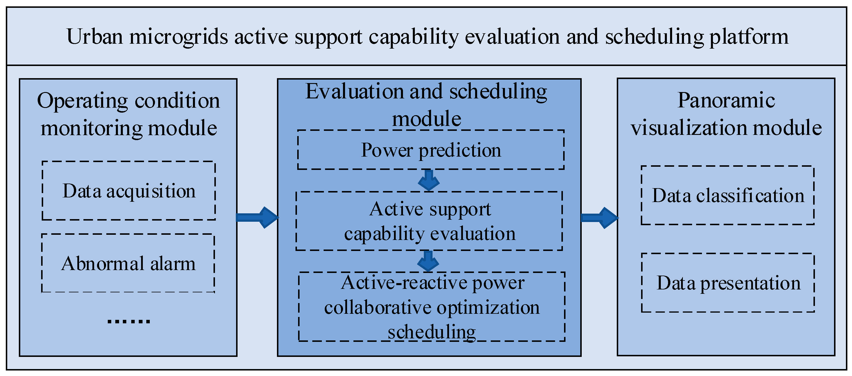
  • The active support capability evaluation and scheduling platform for urban microgrids is constructed. Through the operation condition monitoring module of the platform, the platform operator can obtain the real-time or historical operation data of distributed resources, providing data support for subsequent work.
  • An evaluation model of the active support capability of urban microgrids is established. Some technical indicators are proposed for the active and reactive power support capabilities of urban microgrids to systematically evaluate the overall active support capability of urban microgrids, preparing the data basis and boundary conditions for the scheduling function.
  • An active–reactive power coordinated optimization scheduling method for urban microgrids, considering the operating characteristics of distributed resources and incorporating an SOP, is proposed to obtain the optimal scheduling strategy. Based on the strategy, the operating costs of urban microgrids are reduced and the voltage deviation rate for urban microgrids is suppressed.

2. Evaluation and Control Platform for the Active Support Capability of Urban Microgrids

The evaluation and scheduling platform for the active support capability of urban microgrids is composed of an operation condition monitoring module, evaluation and scheduling module, and panoramic visualization module. Based on database management software and the software support platform, it realizes the monitoring of the operation status of urban microgrids and realizes the control function of active support ability evaluation and optimal dispatching of microgrids by accessing the real-time operation data of distributed resources, such as distributed PVs and distributed ESs, to provide technical support services for the normal and economic operation of urban microgrids. The platform architecture is shown in Figure 1.

2.1. Operation Condition Monitoring Module

The operation condition monitoring module includes graphics and parameter maintenance, data acquisition and analysis processing, event and alarm processing, micro-grid data access and control, and terminal data monitoring functions. It is mainly responsible for the parameter setting of distributed resources in the urban microgrid, data acquisition, and abnormal alarm on the microgrid side. Other auxiliary services provide data support for the evaluation and control module and can transmit the processed accurate data to the evaluation and control module to participate in simulation analysis and calculation.

2.2. Evaluation and Scheduling Module

The evaluation and scheduling module consists of three functional modules: distributed resource power prediction, active support capability evaluation, and active and reactive power collaborative optimization scheduling. Among them, the distributed resource power prediction function can obtain the historical time series data of distributed resources, such as distributed PVs and TCLs transmitted from the operating condition monitoring module, and accurately predict the output or load demand of distributed resources contained in the microgrid in the next 24 h through the prediction model in the module.
The active support capability evaluation function is divided into the active support capability evaluation module and the reactive support capability evaluation module. According to the predicted active power output results of distributed resources, the active power support capability evaluation module calculates the evaluation index through the active power support capability evaluation model embedded in the module and systematically evaluates the active power support capability for distributed resources in the region to the whole urban microgrid. The reactive power support capability evaluation module accepts the relevant reactive power prediction results. According to the reactive power support capability evaluation model, the upper and lower limits of the voltage regulation capacity of each distributed resource in the active–reactive power coordinated optimization regulation are calculated. The voltage support degree of each distributed resource node to the voltage-exceeding node in the microgrid during the active–reactive power coordinated optimization regulation is evaluated, and the reactive power support capability for the distributed resources in the region of the overall urban microgrid is obtained.
The active and reactive power collaborative optimization scheduling function comprehensively considers the distributed resources, such as distributed PVs, ESs, and EVs, in the urban microgrid. The prediction data of the distributed resource power prediction module is used as the input, and combined with the evaluation results of the active support capability evaluation module, the active and reactive power collaborative optimization scheduling method for urban microgrids embedded in the module is implemented. The purpose is to optimize the distribution of active power and reactive power in microgrids so that the distributed resources in urban microgrids can operate reasonably and coordinately, reduce the impact of the volatility and uncertainty of renewable energy on the operation of urban microgrids under high permeability, and improve power quality.

2.3. Panoramic Visualization Module

The panoramic visualization module mainly involves the real-time data display and monitoring of the simulation results calculated by the evaluation and control module, including the displayable resource list of the three functional modules of distributed resource power prediction, active support capability evaluation, and active and reactive power collaborative optimization scheduling. By selecting different distributed resources, the measurement or calculation data types of the corresponding resources can be displayed, and the prediction, evaluation, and scheduling results obtained by the simulation calculation are classified according to the results of distributed resource data information, node load information, and evaluation index information and are displayed in real time in the form of digital information or a data curve.

3. Active Support Capability Assessment

As the core algorithm of distributed resource power prediction and the active support capability evaluation module, the active support capability evaluation model is responsible for the output or load prediction of distributed resources, as well as the evaluation of the active support capability and reactive support capability of the whole urban microgrid.

3.1. Active Power Support Capability Evaluation
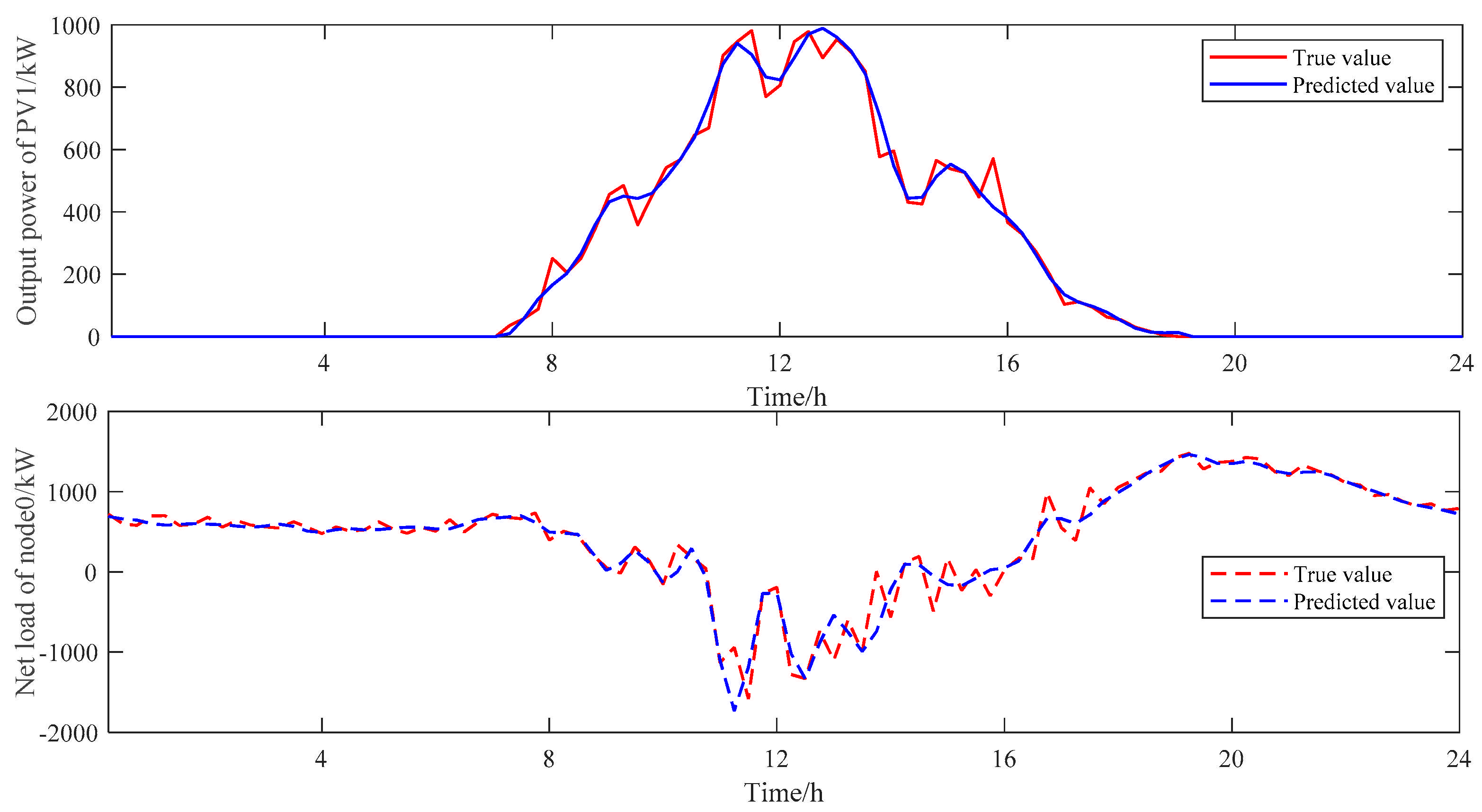
The evaluation of the active power support capability is divided into two parts: the prediction model and the active power support capability evaluation model. The prediction model predicts the output of distributed resources and the load of the microgrid through historical time series data and provides data support for the active power support capability evaluation model. The active power support capability evaluation model partially systematically evaluates the overall active power support capability of the microgrid.

3.1.1. BiLSTM Model

In urban microgrids, the output of distributed energy resources including PVs and the demand of electric loads exhibit distinct temporal characteristicscs, showing a certain law of change with time. Therefore, based on BiLSTM, a distributed resource output prediction model is constructed, and the output characteristics of distributed resources in the urban microgrid are mined using BiLSTM’s strong timing feature capture ability. LSTM can effectively learn and remember long-term time dependence, while BiLSTM is improved on the basis of LSTM, which is composed of forward LSTM and backward LSTM. Through this two-way structure, it can extract time series information from past and future directions and improve the prediction model’s ability to understand time characteristics [14]. As a result, a more complete time connection can be obtained to enhance the accuracy of distributed resource output prediction in the microgrid. The basic LSTM is composed of the forgetting gate f t , input gate i t , and output gate o t . Through the gate mechanism, LSTM can selectively remember valuable information or forget useless information. The specific LSTM can be represented by Equations (1)–(6):
f t = σ ( W f · [ h t 1 , x t ] + b f )
i t = σ ( W i · [ h t 1 , x t ] + b i )
C ˜ t = tanh ( W C · [ h t 1 , x t ] + b C )
C t = f t · C t 1 + i t · C ˜ t
o t = σ ( W o · [ h t 1 , x t ] + b o )
h t = o t · tanh ( f t · C t 1 + i t · C ˜ t )
where x t and h t denote the input and hidden states at time t, respectively; C ~ k and C k represent the candidate cell state and the current cell state, respectively; σ · and t a n h · are activation functions; and W f , W i , W o , W C and b f , b i , b o , b C are the weight matrix and the bias matrix of the corresponding gate, respectively.
Based on the original LSTM, BiLSTM combines forward LSTM and backward LSTM to obtain time series information from two directions and mine time features. The related calculation process of BiLSTM can be represented by Equations (7)–(9):
h t = LSTM ( x t , h t 1 )
h t = concat ( h t , h t )
where h t and h t are the forward and backward LSTM outputs at time t, respectively; L S T M · represents the propagation process of (1)–(6); and c o n c a t · denotes the splicing operation.
The relevant meteorological data and historical sequence data screened by the maximum mutual information coefficient method are used to form a feature matrix as the input of the prediction model based on BiLSTM. The active power P ~ i , t L o a d of the node load, the reactive power Q ~ i , t L o a d of the node load, and the output data P ~ i , t m of the distributed resources with different prediction requirements are obtained for a total of 96 moments in the next 24 h, where m is the type of distributed resource.

3.1.2. Active Power Support Capability Evaluation Model Based on BiLSTM Model

The active power support capability of urban microgrids refers to their ability to maintain and manage active power, which is the key factor for microgrids to ensure that the local load meets the power demand and maintains the normal operation of the system. In urban microgrids, the active power support capability is mainly reflected in the two aspects of power consumption level and power generation level. Therefore, this paper proposes an evaluation index for the two power resources of distributed resources and power load of the urban microgrid to measure the active power support capability in the microgrid area.
Using the prediction model based on BiLSTM established in the previous section, the point prediction of PVs and power load of the microgrid is carried out, respectively, and the prediction results of 96 time nodes in the next 24 h are obtained. Then, the confidence interval range and point fluctuation amplitude are proposed as two evaluation indexes of the active power support capability. Specifically, due to various human and environmental factors, there is a certain degree of uncertainty in the prediction results of distributed resources and loads. The range of this uncertainty can be expressed as a fuzzy chance constraint and expressed in the form of a confidence interval at the confidence level α . The confidence interval range can represent the uncertainty range of the prediction results, as shown in Equation (10):
P ˜ i , t M e i , t M 3 π σ i , t M ln α 1 α P ˜ i , t M e i , t M + 3 π σ i , t M ln α 1 α
where M represents the type of distributed resource or load; e i , t M and σ i , t M denote the mean and standard deviation of M at time t of node i, respectively; and P ~ i , t M denotes the active power range of M located at time t of node i. It should be noted that the confidence level α can change dynamically in the range of [ 0.5 , 1 ) to ensure the feasibility of the confidence interval. The obtained confidence interval quantifies the level of uncertainty in photovoltaic output and load demand forecasting. A larger interval range indicates greater fluctuation amplitudes during that time period. The upper and lower bounds of the confidence interval will serve as the boundary conditions for subsequent uncertainty scenario generation to avoid the occurrence of extreme operating scenarios. In addition, the point fluctuation amplitude is the first derivative of the point prediction result, which is used to reflect the stability of the prediction data in a certain period of time.

3.2. Reactive Power Support Capability Evaluation

The reactive power support capability of urban microgrids refers to their ability to manage and regulate reactive power to maintain system voltage stability, and reactive power is critical to maintaining the voltage level of the power system. Compared with the regulation of active power, the regulation cost of reactive power is lower and the impact on the user side is smaller. Therefore, the regulation of reactive power is usually selected as the voltage regulation method. The support degree of reactive power regulation to node voltage and the reactive power regulation ability are proposed as evaluation indexes to measure the reactive power support ability of nodes where distributed resources are located in the microgrid area.

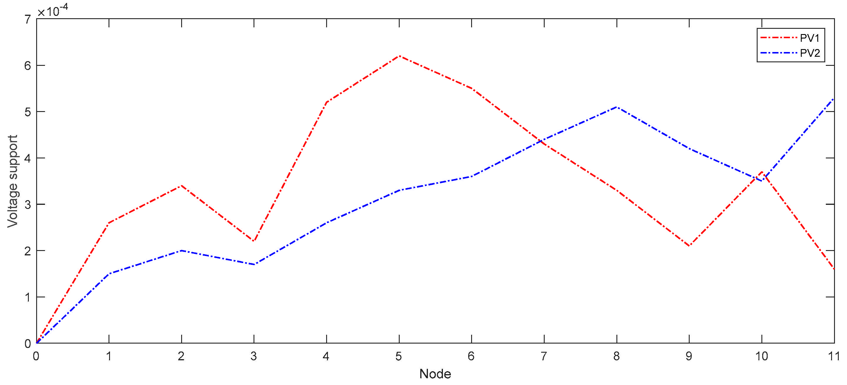
3.2.1. Voltage Support Degree

The voltage support degree can reflect the degree of voltage change of related nodes caused by reactive power change of distributed resources in the microgrid. Combining the active voltage sensitivity matrix S ( N × M ) , t P and the reactive voltage sensitivity matrix S ( N × M ) , t Q , the voltage support degree can be expressed as shown in Equation (11):
Δ U 1 , t Δ U 2 , t Δ U N , t = S ( N × M ) , t P Δ P 1 , t Δ P 2 , t Δ P M , t + S ( N × M ) , t Q Δ Q 1 , t Δ Q 2 , t Δ Q M , t
where U i , t , P i , t , and Q i , t represent the voltage, active power, and reactive power at time t of node i, respectively; and N and M are the nodes and the total number of PVs in the urban microgrid, respectively.

3.2.2. Reactive Power Regulation Ability

Urban microgrids generally include distributed PVs and ESs, which have considerable reactive power adjustment capabilities. Among them, PVs can emit or absorb reactive power due to the existence of an inverter to achieve the effect of regulating reactive power. The reactive power regulation ability of PVs is affected by the capacity of the inverter. When the active power output is constant, the maximum adjustable reactive power Δ Q i , t , m a x P V and the minimum adjustable reactive power Δ Q i , t , m i n P V can be represented by Equations (12) and (13):
Δ Q i , t , max PV = S i PV 2 P i , t PV 2 Q i , t PV
Δ Q i , t , min PV = S i PV 2 P i , t PV 2 Q i , t PV
where P i , t P V and Q i , t P V are the active and reactive power outputs of PVs at time t of node i, respectively; and S i P V is the inverter capacity of PVs at node i.
The reactive power regulation ability of ESs is also affected by their capacity and the maximum adjustable reactive power Δ Q i , t , m a x E S and minimum adjustable reactive power Δ Q i , t , m i n E S can also be expressed in a similar form, as shown in Equations (14) and (15):
Δ Q i , t , max ES = S i ES 2 P i , t ES 2 Q i , t ES
Δ Q i , t , min ES = S i ES 2 P i , t ES 2 Q i , t ES
where P i , t E S and Q i , t E S are the active power and reactive powers stored at time t of node i, respectively; and S i E S is the capacity of ESs at node i.
The overall reactive power adjustment capability of urban microgrids can be represented by Equations (16) and (17):
Δ Q i , t , max Tol = Δ Q i , t , max PV + Δ Q i , t , max ES
Δ Q i , t , min Tol = Δ Q i , t , min PV + Δ Q i , t , min ES

4. Active–Reactive Power Collaborative Optimization Scheduling

Urban microgrids with a high proportion of renewable energy face significant challenges in maintaining voltage stability and optimizing power flow distribution. Traditional models that optimize active or reactive power independently cannot simultaneously ensure both secure operation and low network losses or operating costs of microgrids. To address this issue, an active–reactive power coordinated optimization model is proposed, which comprehensively considers the operational characteristics of heterogeneous distributed energy resources and an SOP to achieve coordinated control for microgrids. This section uses the results predicted by the BiLSTM-based prediction model and the evaluation results of the active support capability to perform day-ahead active–reactive power coordinated optimization scheduling for urban microgrids.

4.1. Objective Function

With the rapid development of urban microgrids, the distributed resources contained in them are becoming more and more diversified. Common resources include PVs, ESs, EVs, and TCLs. The rational use of these distributed resources can improve the operating conditions of urban microgrids [19]. At the same time, considering the economy of the microgrid, a mathematical model of active–reactive power collaborative optimization of urban microgrids is established with the minimum operating cost F 1 and the minimum voltage offset F 2 as the objective functions. The comprehensive objective function F considering different weight coefficients k is expressed as shown in Equation (18):
min F = k 1 F 1 + k 2 F 2
Specifically, the operating cost F 1 consists of three parts: the network loss cost f 1 , the running cost f 2 of distributed resources, and the penalty cost f 3 of the demand response, as shown in Equations (19)–(24):
f 1 = t = 1 T i = 1 N j = 1 N G i j , t U i , t 2 + U j , t 2 2 U i , t U j , t cos θ i j , t
where U i , t represents the voltage amplitude at time t of node i; and G i j , t and θ i j , t represent the conductance and phase angle of line ij at time t, respectively.
f 2 = t = 1 T i Ω PV C i , t PV + i Ω ES C i , t ES + i Ω SOP C i , t SOP
C i , t PV = ρ PV · P i , t PV
C i , t ES = ρ ES · P i , t ES
C i , t SOP = ρ SOP · P i , t SOP
where C i , t P V , C i , t E S , and C i , t S O P represent the operating costs of PVs, ESs, and the SOP, respectively; ρ P V , ρ E S , and ρ S O P are the unit power generation costs of PVs, the unit operation costs of ESs, and the unit regulation cost of the SOP, respectively; P i , t P V and P i , t E S are the active power outputs of PVs and energy storage at time t of node i, respectively; P i , t S O P is the active power regulation of the SOP at time t of node i; and Ω P V , Ω E S , and Ω S O P are the sets of PVs, energy storage, and the SOP, respectively.
f 3 = t = 1 T λ t PV i Ω PV Δ P i , t PV + λ t SOP i Ω OPQ P i , t SOP + λ t EV i Ω EV Δ P i , t EV + λ t TCL i Ω TCL Δ P i , t TCL
where Δ P i , t P V , Δ P i , t E V , and Δ P i , t T C L are the active power adjustments of PVs, EVs, and TCLs at node i and time t, respectively; Ω E V and Ω T C L represent the sets of EVs and TCLs, respectively; and λ t P V , λ t S O P , λ t E V , and λ t T C L are the light abandonment penalty costs of PVs at time t, the lifetime degradation cost of the SOP, and the adjustment compensation costs of EVs and TCLs, respectively. Therefore, the operating cost F 1 can be expressed by the above three parts with different weight coefficients m, as shown in Equation (25):
F 1 = m 1 f 1 + m 2 f 2 + m 3 f 3
In addition, the voltage deviation rate F 2 can be represented by Equation (26):
F 2 = i = 1 N U i , t U i , N U i , N
where U i , N represents the rated voltage value of node i.

4.2. Constraint Condition

4.2.1. Power Flow Constraints

The DisFlow power flow equation is used to represent the power flow constraints and can be expressed by Equations (27)–(32):
Δ P j , t + i L j P i j , t R i j · l i j , t k J j P j k , t = 0 Δ Q j , t + i I j Q i j , t X i j · l i j , t k K j Q j k , t = 0
Δ P i , t = P i , t PV + P i , t ES P i , t EV P i , t TC P i , t Load Δ Q i , t = Q i , t PV + Q i , t ES Q i , t Load
U i , t U j , t = 2 R i j P i j , t + X i j Q i j , t l i j , t R i j 2 + X i j 2
2 P i j , t 2 Q i j , t l i j , t U i , t 2 l i j , t + U i , t
U i , min U i , t U i , max
P i j , t 2 + Q i j , t 2 S i j 2
where Δ P i , t and Δ Q i , t are the active and reactive powers injected by node i at time t, respectively; P i j , t and Q i j , t represent the active power and reactive power flowing through the line ij at time t, respectively; S i j is the capacity of line i j ; l i j , t denotes the square of the line i j current; R i j and X i j are the resistance and reactance of line i j , respectively; Q i , t E S is the reactive power generated by ES; and P i , t L o a d and Q i , t L o a d are the active power and reactive power consumed by the load of node i at time t, respectively.

4.2.2. Photovoltaic Constraints

The distributed PVs in the microgrid can adjust the active and reactive power outputs through the inverter to improve the power flow. The related constraints can be represented by Equations (33)–(37):
P i , t PV 2 + Q i , t PV 2 S i PV 2
0 P i , t PV P i , t , max PV
0 Q i , t PV Q i , t , max PV
0 Δ P i , t PV Δ P i , t , max PV
Δ Q i , t , min PV Δ Q i , t PV Δ Q i , t , max PV
where P i , t , m a x P V and Q i , t , m a x P V represent the upper limits of the active and reactive power outputs of PVs, respectively; and P i , t , m a x P V is the upper limit of PVs’ active power reduction.

4.2.3. Energy Storage Constraints

ESs interact with the microgrid through charging or discharging to achieve the effect of balancing the power flow, which can significantly improve the stability and reliability of the microgrid operation. The related constraints can be represented by Equations (38)–(42):
P i , t ES 2 + Q i , t ES 2 S i ES 2
P i , t , ch , min ES P i , t , ch ES P i , t , ch , max ES
P i , t , dis , min ES P i , t , dis ES P i , t , dis , max ES
E i , t , soc ES + P i , t , ch ES η ch ES Δ t P i , t , dis ES η dis ES Δ t = E i , t + 1 , soc ES
E i , t , soc , min ES E i , t , soc ES E i , t , soc , max ES
where P i , t , c h E S and P i , t , d i s E S are the charge and discharge powers of ESs, respectively; P i , t , c h , m i n E S / P i , t , c h , m a x E S and P i , t , d i s , m i n E S / P i , t , d i s , m a x E S are the upper and lower limits of the charge and discharge powers of ESs, respectively; E i , t , S O C E S , E i , t , S O C , m i n E S , and E i , t , S O C , m a x E S represent the upper and lower bounds of the stored energy and the stored energy of ESs, respectively; and η c h E S , η d i s E S , and S i E S represent the charge–discharge efficiency and capacity of ESs, respectively.

4.2.4. Electric Vehicle Constraints

EVs can participate in the interaction of microgrids under reasonable control strategies, reduce load during peak load, or increase charging power during trough load, so as to achieve peak load shifting and obtain economic benefits. The related constraints can be represented by Equations (43)–(45):
P i , t , min EV P i , t EV P i , t , max EV
E i , t , soc , min EV E i , t , soc EV E i , t , soc , max EV
E i , t , soc EV + P i , t , ch EV η ch EV Δ t = E i , t + 1 , soc EV
where P i , t E V and E i , t , S O C E V represent the charging power and storage energy of EVs, respectively; P i , t , m i n E V / P i , t , m a x E V and E i , t , S O C , m i n E V / E i , t , S O C , m a x E V represent the upper and lower limits of the charging power and storage energy of EVs, respectively; and η c h E V is charging efficiency of EVs.

4.2.5. Temperature Control Load Constraint

As a typical adjustable load, TCLs can reduce or increase the active load by adjusting the setting temperature or start–stop time without affecting the user’s comfort. Their flexible adjustment ability is shown in Equations (46)–(48):
P i , min TCL P i , t TCL P i , max TCL
T base Δ T TCL T i , t in T base + Δ T TCL
T i , t in = T i , t in e Δ t / λ re R ca + 1 e Δ t / λ re R ca T i , t out λ re η TCL 1 e Δ t / λ re R ca P i , t TCL
where P i , t T C L represents the operating power of TCLs; P i , m i n T C L and P i , m a x T C L are the upper and lower limits of the operating power of TCLs, respectively; T b a s e and T T C L represent the reference value and dead zone value of the indoor temperature, respectively; T i , t i n and T i , t o u t represent the indoor temperature and outdoor temperature, respectively; and λ r e , R c a , and η T C L are the equivalent thermal resistance and heat capacity of TCLs and the heating performance coefficient, respectively.

4.2.6. SOP Constraints

A flexible intelligent switch SOP is considered to participate in the active and reactive power collaborative optimization of microgrids. An SOP is a new type of power electronic device, which can optimize the power flow distribution by adjusting and controlling the transmission of active power and reactive power of the connected lines, so as to replace the traditional contact switch to improve the operation state of the distribution network. Considering SOPs in the problem of active and reactive power optimization of microgrids can significantly improve the power flow distribution and voltage fluctuation of microgrids. The constraints are shown in Equations (49)–(51):
P i , t SOP + P j , t SOP + η i j SOP P i , t SOP 2 + Q i , t SOP 2 + η i j SOP P j , t SOP 2 + Q j , t SOP 2 = 0
P i , t SOP 2 + Q i , t SOP 2 + η i j SOP P i , t SOP 2 + Q i , t SOP 2 S i j SOP 2 P j , t SOP 2 + Q j , t SOP 2 + η i j SOP P j , t SOP 2 + Q j , t SOP 2 S i j SOP 2
Q i , min SOP Q i , t SOP Q i , max SOP Q j , min SOP Q j , t SOP Q j , max SOP
where P i , t S O P , P j , t S O P , Q i , t S O P , and Q j , t S O P are the active powers and reactive powers injected by node i and node j connected at both ends of the SOP, respectively; Q i , m i n S O P , Q i , m a x S O P , Q j , m i n S O P , and Q j , m a x S O P represent the minimum and maximum reactive powers allowed to be injected by node i and node j connected at both ends of the SOP, respectively; and η i j S O P and S i j S O P represent loss coefficient and capacity of the SOP, respectively.
In addition, the capacity constraints of some distributed resources, such as (32), are non-convex, which will increase the difficulty of solving the optimization problem. Therefore, these constraints are transformed into convex constraints by piecewise linear representation. Taking the capacity constraint of PVs as an example, its piecewise linear representation is shown in Equation (52):
P i , t PV · cos 2 k π N + Q i , t PV · sin 2 k π N S i , t PV · cos π N , k [ 1 , N ]

4.3. Introduction of Stochasticity

In urban microgrid optimal scheduling, the uncertainties in photovoltaic output and load demand are critical factors affecting both system security and economic performance. Photovoltaic generation exhibits high intermittency and variability due to its significant dependence on weather conditions, while load demand shows stochastic fluctuations influenced by consumer behavior. Neglecting these uncertainties may compromise the microgrid’s secure and economic operation. In this context, a scenario-based stochastic programming approach is adopted to model photovoltaic output and load demand uncertainties. Specifically, the prediction errors for photovoltaic output or load demand in each time period are treated as random variables with known probability distribution functions e.g., Gaussian distribution. Through Monte Carlo simulation, the prediction errors Δ P i , t , s P V , E and Δ P i , t , s L o a d , E are sampled from their respective probability distribution functions. Consequently, the actual photovoltaic output P i , t , s P V and load demand P i , t , s L o a d of node i at time t in scenario s can be expressed in terms of their predicted values P ~ i , t , s P V and P ~ i , t , s L o a d , as shown in Equations (53) and (54):
P i , t , s PV = P ˜ i , t PV + Δ P i , t , s PV , E
P i , t , s Load = P ˜ i , t Load + Δ P i , t , s Load , E
where s ψ , and ψ denote the scenario sets. It should be noted that for each scenario, the generated photovoltaic output or load demand must be constrained within the confidence interval to avoid the creation of extreme scenarios.
The scenario probabilities are determined using the roulette wheel selection mechanism. Specifically, for each prediction variable, its probability distribution function is discretized into multiple intervals centered around zero mean, with each interval width equal to the standard deviation σ. The probability of each interval is calculated by integrating the probability distribution function over its range, followed by normalization to ensure the total probability sums to 1. For each prediction variable, a random number is drawn from the probability distribution function, and a set of binary parameters is employed to indicate the selected state. If the random number falls within interval l, its associated binary parameter is set to 1, and the probability of this interval is assigned as the occurrence probability of the scenario. Simultaneously, all other binary parameters corresponding to different intervals are set to 0. This process is iteratively repeated until scenarios are generated for all scheduling periods of photovoltaic output or load demand. Consequently, each scenario represents a possible realization of 24 h photovoltaic generation or load demand in the microgrid. Since the generation processes for different prediction variables are independent events, the normalized occurrence probability of each scenario π s can be computed as Equation (55):
π s = t T i F PV l L δ i , l , t , s PV π i , l , t , s PV i F Load l L δ i , l , t , s Load π i , l , t , s Load s ψ t T i F PV l L δ i , l , t , s PV π i , l , t , s PV i F Load l L δ i , l , t , s Load π i , l , t , s Load
where δ i , l , t , s P V , δ i , l , t , s L o a d , π i , l , t , s P V , and π i , l , t , s L o a d represent the binary parameters and probabilities of interval l associated with each predicted photovoltaic output and load demand at time t in scenario s, respectively; T and L are the sets of scheduling periods and discretized intervals, respectively; and F P V and F L o a d denote the sets of PVs and loads, respectively.
Based on the generated scenarios, the stochastic optimization model for determining active–reactive power coordinated optimization strategies in urban microgrids is updated, as shown in Equation (56):
min F = s ψ π s ( k 1 F 1 , s + k 2 F 2 , s ) s . t .   ( 27 ) - ( 32 ) , ( 33 ) ( 48 ) , ( 49 ) - ( 51 )
where constraints (27)–(32) represent the power flow constraints, constraints (33)–(48) characterize the operational constraints of distributed energy resources within the microgrid, and constraints (49)–(51) describe the physical model constraints of the SOP.
So far, the construction of an active–reactive power collaborative optimization model for urban microgrids with a high proportion of renewable energy has been completed. Since the optimization model is a convex model as a whole, it can be solved quickly and efficiently using commercial solvers such as Gurobi, and the solution results are transmitted to the panoramic visualization module described in Section 2 for data display.

5. Case Studies

5.1. Base Data

The active–reactive power collaborative optimization method proposed in this paper was tested in an urban microgrid with a high proportion of renewable energy in Guangdong Province, China. The equivalent topology is shown in Figure 2, with numbers 1–11 representing urban microgrid nodes. The microgrid consisted of 12 nodes and 12 branches, with the impedance parameters derived from actual system data. The microgrid operated at a 10 kV voltage level with permissible voltage fluctuations ranging from 0.95 p.u. to 1.05 p.u., while the line capacities were set at 10 MVA. The microgrid contained distributed resources including 2 PVs, 2 ESs, 2 EVs, 1 TCL, and 1 SOP. Specifically, PVs with installed capacities of 2.6 MW and 2.05 MW were connected at node 5 and node 11, respectively. Nodes 3, 6, and 10 were equipped with 2 EVs and 1 TCL, all capable of responding to scheduling strategies through active power adjustment. ESs with capacities of 0.3 MW/0.6 MWh were installed at nodes 5 and 11. The SOP was connected between node 2 and node 9 with a capacity of 0.2 MW. The training data for the active support capability evaluation module came from actual historical operation data of the urban microgrid, including 15 min resolution historical time series data of PV output and load demand. Additionally, the required historical meteorological data were obtained from a professional meteorological data platform to ensure data reliability [21]. The proposed method was implemented using Python/PyTorch v2.4.0 for the prediction model, trained with the Adam optimizer, Python/CVXPY v2.4.0 was used for the optimization scheduling model, and it was solved using the Gurobi v10.0.2 solver.

5.2. Active Support Capability Assessment Results

The evaluation of the active support capability was divided into two parts: active support capability evaluation and reactive support capability evaluation. Figure 3 shows the prediction results of the output of PV1 and the net load of node 0 in the microgrid based on the BiLSTM-based prediction model on a certain day and quantitatively evaluates the active power support capacity of the urban microgrid based on the prediction results, as shown in Table 1. The maximum confidence interval range indicated that the photovoltaic output or load demand exhibited significant fluctuations during peak periods, suggesting that the dispatch system needed to reserve more flexible resources to cope with sudden power variations. Conversely, the minimum confidence interval range under low-power conditions reflected higher stability, allowing the microgrid to reduce its backup capacity allocation. From Figure 3, it can be seen that both the photovoltaic output prediction results and the load prediction results of the nodes are in line with their actual change trends and achieved the expected results. In addition, taking RMSE and MAE as the evaluation indexes of prediction accuracy, the comparison results with other prediction methods are shown in Table 2. Compared with GRU [12], LSTM [13], RNN [22], Transformer [23], and GCN [24], the proposed BiLSTM-based prediction model reduced RMSE and MAE by an average of 15.82% and 13.24%, respectively. These results demonstrated that the BiLSTM-based prediction model achieved superior performance in both photovoltaic output and load demand prediction, exhibited enhanced feature extraction capability for time series data, and more effectively captured the relationship between either photovoltaic output or load demand and temporal variations. Additionally, using the prediction results as baselines, multiple plausible scenarios for photovoltaic output and load demand were generated to represent the uncertainties of distributed energy resources and load demands in the urban microgrid, as shown in Figure 4. In the stochastic optimization model, 10,000 initial scenarios were first generated and subsequently reduced to 100 scenarios through the backward reduction algorithm [25], maintaining effective uncertainty representation while significantly reducing computational burden.
The voltage support of the two PVs located at node 6 and node 11 to the urban microgrid is shown in Figure 5. It was found that the voltages of the nodes in the microgrid were affected by the PVs’ reactive power output, and the closer the node was to the PV, the greater the impact, and as the distance increased, the impact gradually decreased.
Figure 6 shows the overall reactive power regulation capability of the urban microgrid, including the reactive power adjustable capacity of PVs and ESs. It can be found in the diagram that the reactive power regulation ability of the microgrid is affected by the active power output of PVs and ESs, which decreases with the increase of active power output. For PVs, the active output at night is almost 0, and the reactive power regulation ability is almost equal to their own installed capacity.

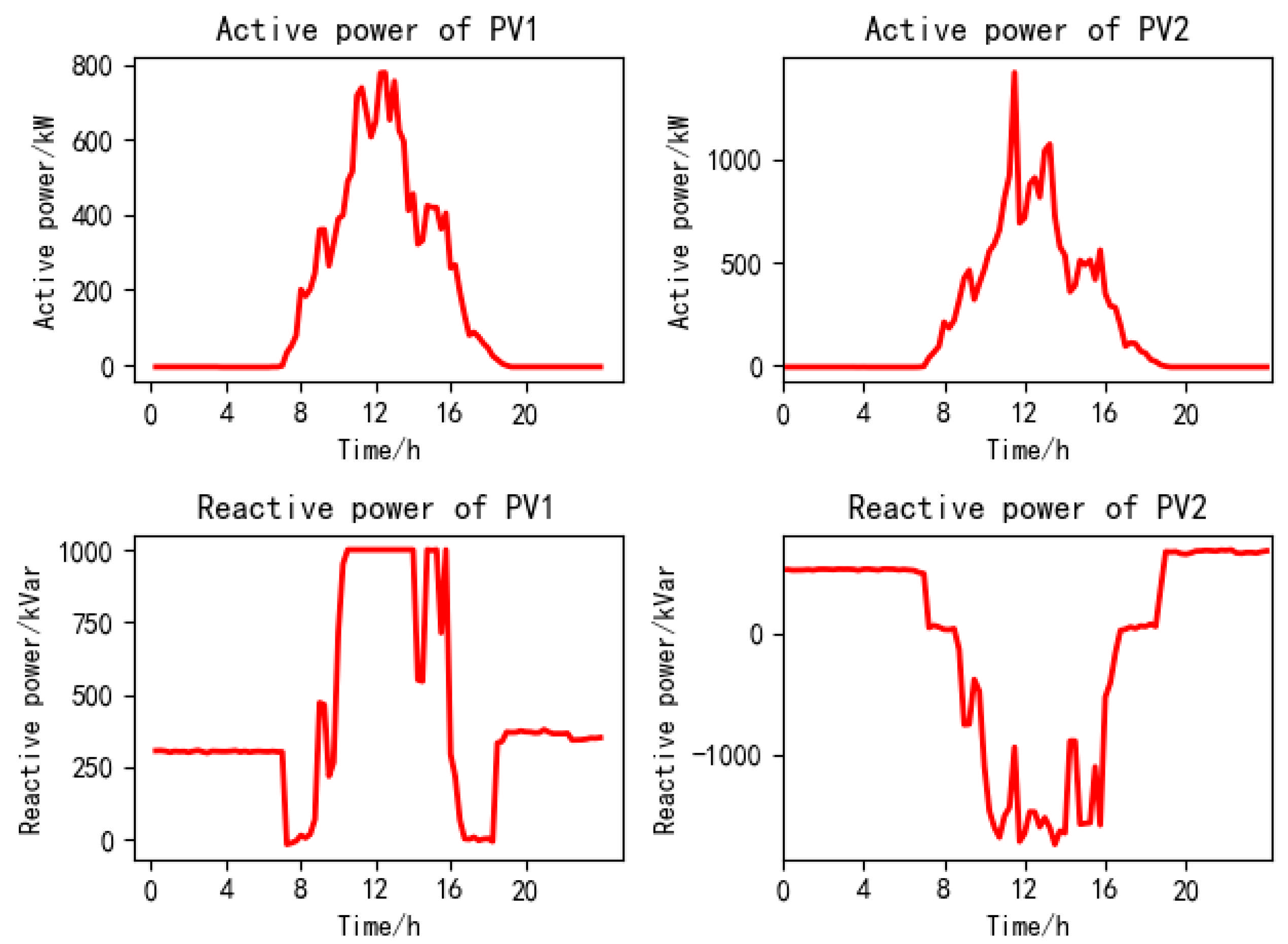
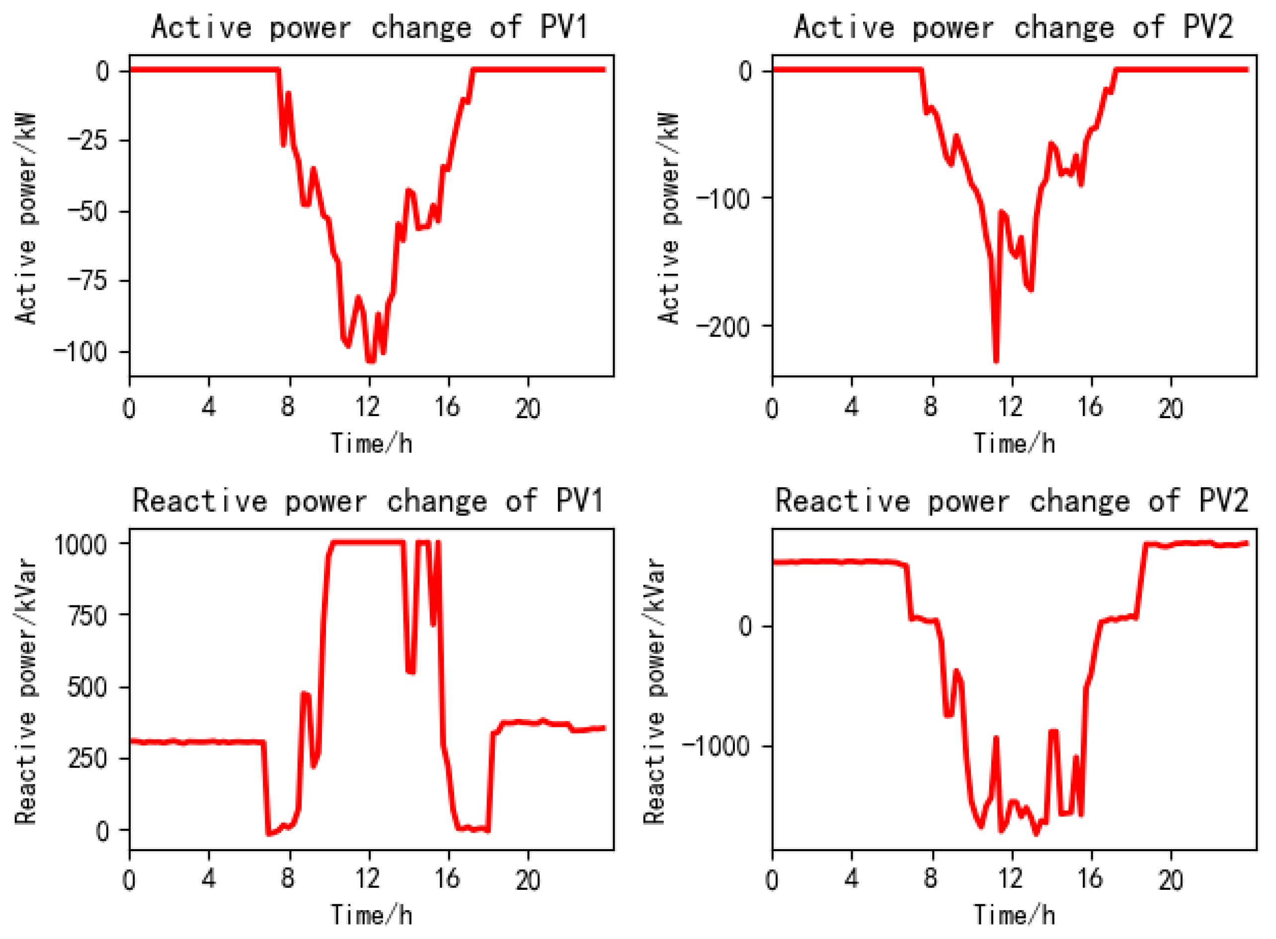
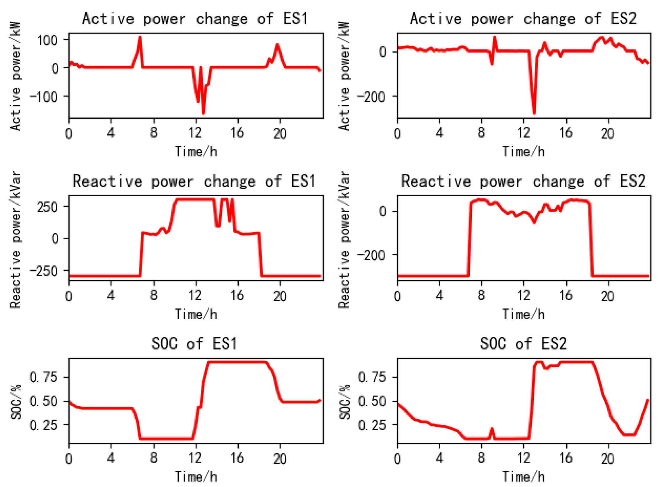
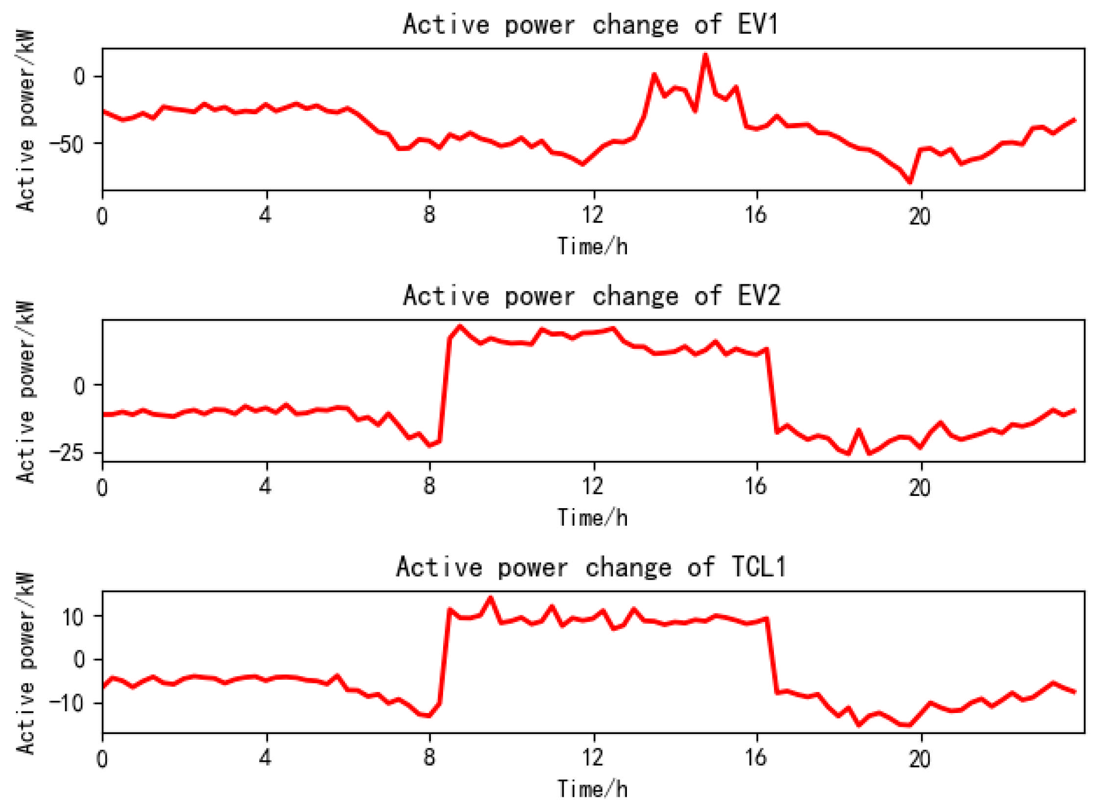
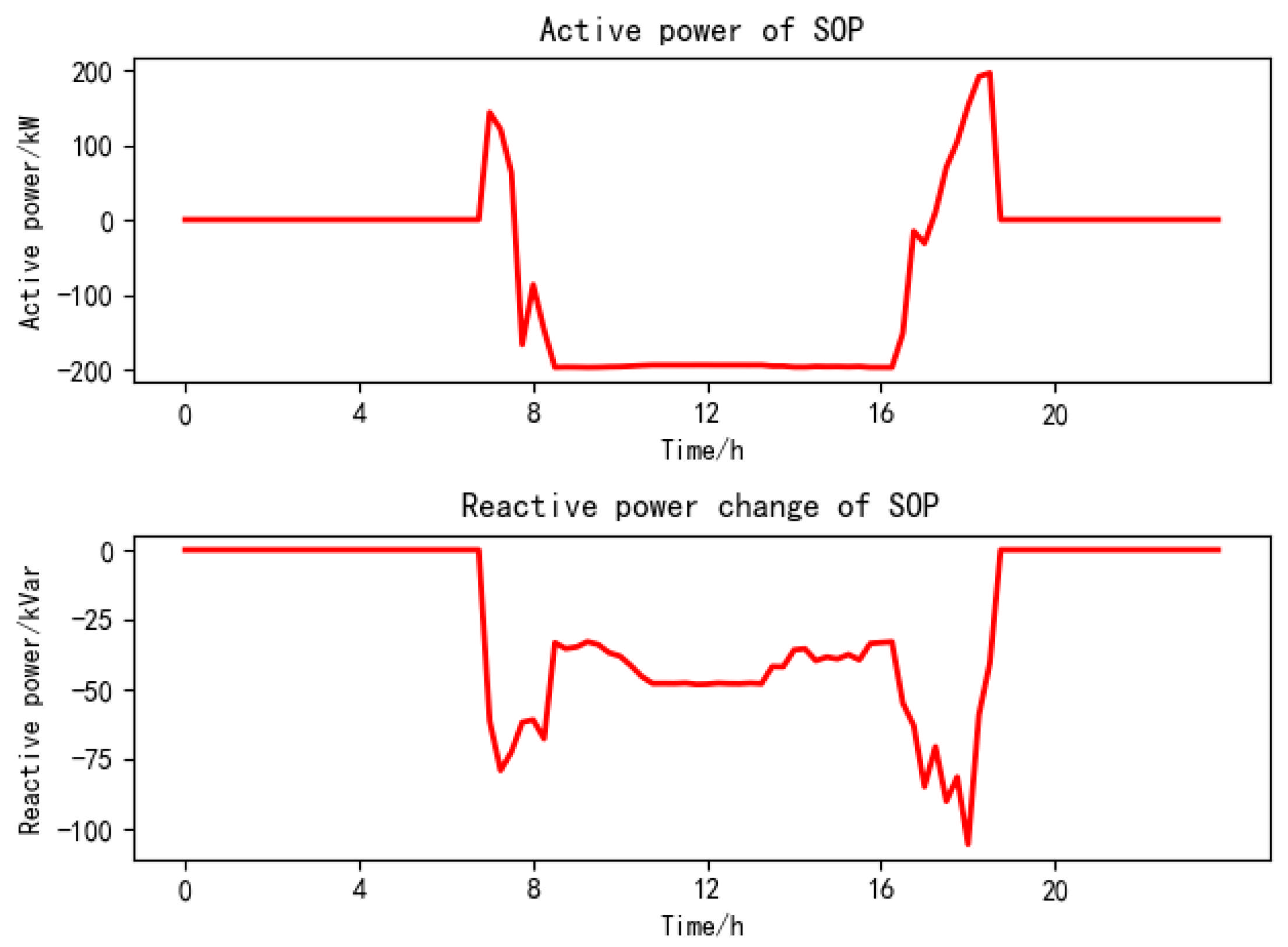
5.3. Collaborative Active–Reactive Power Optimization Scheduling Results

Figure 7 and Figure 8 show the active and reactive power outputs of two PVs located at node 5 and node 11 after optimization, and the changes of their active and reactive power outputs after optimization. It can be found that there is no active power output of the PVs before sunrise and after sunset, and with the increase in solar irradiation intensity, the active power output of the PVs gradually increases until the peak at noon and then gradually decreases. In addition, due to the existence of inverters, the PVs can provide reactive power for the microgrid to participate in power regulation to ensure the normal operation of the microgrid. When photovoltaic power is generated, the microgrid may have power reversal and voltage over-limits. Currently, in order to ensure the safe operation of the microgrid, it is necessary to reduce the output of some photovoltaics and rationally allocate the power flow inside the microgrid by regulating other distributed resources. While ensuring safety, the amount of light discarded should be reduced as much as possible to achieve the effect of improving the consumption rate of renewable energy.
Figure 9, Figure 10 and Figure 11 show the output curves of the ESs, EVs, TCL, and the SOP under active–reactive power optimization scheduling. It can be seen from Figure 9 that before sunrise and after sunset, the load of the microgrid is in a clear deficit state. At this time, ESs provide part of the active power for the microgrid through discharge, and at the same time, they provide considerable reactive power. When photovoltaic power is generated, the microgrid cannot consume so much power in time, so the ESs store the redundant power at this time, and the SOC increases significantly, which provides support for the subsequent power regulation of the microgrid. Figure 10 shows that under the reasonable control strategy, the EVs and TCL can increase or reduce the active power consumption in the microgrid by increasing or reducing the load, so as to achieve the effect of peak load shifting. In addition, with the change in load and distributed resource output, the SOP can make corresponding dynamic changes. By adjusting the active power and reactive power of its transmission, the SOP can achieve a certain dredging effect on power flow, as shown in Figure 11.
Figure 12 shows the voltage of each node in the microgrid at different times before and after the coordinated optimization of active and reactive powers. It can be observed that if the microgrid is not optimized and regulated, when photovoltaic power is generated, the overall voltage of the microgrid is obviously over-limit, and the nodes near the PVs are seriously over-limit, which will seriously endanger the normal operation of the microgrid. Through a reasonable optimization control strategy, distributed resources such as PVs, EVs, and ESs adjust their output or operating status, optimize the power flow distribution within the microgrid, and constrain the overall voltage of the microgrid within a reasonable range, and the voltage of each node does not exceed the limit. It should be noted that after optimization, not only did the voltage of each node not exceed the limit but also the overall voltage fluctuation range of the urban microgrid was significantly reduced, achieving the expected results.

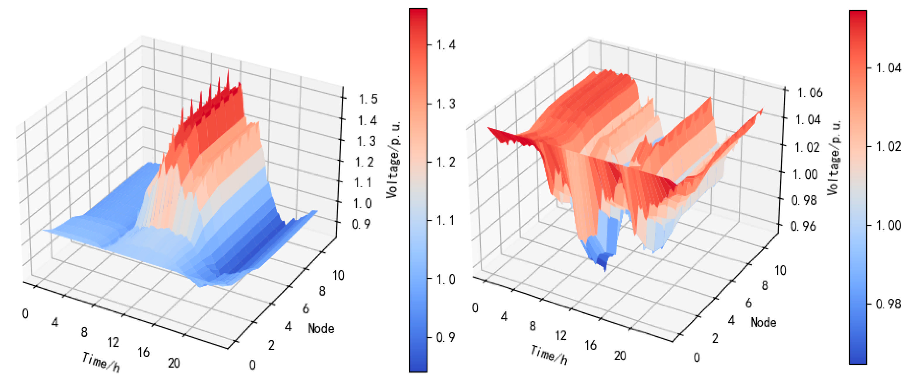
5.4. Comparative Results and Analysis

To validate the feasibility and superiority of the proposed control method, five comparative Schemes were implemented: (1) Scheme 1 adopted the active–reactive power coordinated optimization control method proposed in Section 4, accounting for uncertainties in the urban microgrid; (2) Scheme 2 employed the deterministic optimization model that neither considered distributed energy resources nor incorporated the SOP in the optimization control method; (3) Scheme 3 used the optimization control model proposed in Section 4 without considering uncertainties in the urban microgrid; (4) Scheme 4 implemented the active power single-objective optimization control method in [26]; and (5) Scheme 5 applied the reactive power single-objective optimization control method in [27].
Table 3 compares the comprehensive operational costs and overall voltage deviation rates of the urban microgrids across Schemes 1–5. A comparison between Scheme 1 and Scheme 2 demonstrated that by incorporating distributed energy resources and the SOP into the optimization control, the urban microgrid gained flexible control capabilities to optimize power flow distribution and improve overall voltage fluctuations. The total cost and voltage deviation rate were reduced by 19.86% and 72.49%, respectively. Compared with Scheme 3, Scheme 1’s consideration of uncertainties effectively avoided extreme scenarios and achieved superior operational performance, with reductions in both total cost and voltage deviation rate. The comparison between Scheme 1 and Schemes 4–5 revealed that single-objective optimization focusing solely on active power reduced network losses but achieved only a 2.4% decrease in total cost while increasing the voltage deviation rate by 52.69%. Similarly, reactive power single-objective optimization in Scheme 5 constrained the voltage deviation rate to 3.17% but increased the total cost by 13.71% compared to Scheme 1. In consequence, the proposed active–reactive power coordinated optimization control method for urban microgrids with a high proportion of renewable energy outperformed the other four Schemes in overall operational performance, simultaneously ensuring economic efficiency.

6. Conclusions

Aiming at the normal operation of microgrids with a high proportion of renewable energy, this paper proposes an active–reactive power coordinated optimization control method. The key innovations are as follows: (1) An active support capability evaluation and control platform for urban microgrids is built. The platform is embedded with the algorithm proposed in this paper, which can realize the active support capability evaluation and active–reactive power coordinated optimization control function of urban microgrids while providing data support to ensure the normal operation of microgrids. (2) An evaluation model of the active support capability of urban microgrids is established, which can evaluate the active support capability and reactive support capability of the whole urban microgrid and provide data support and boundary constraints for the dispatching part. (3) Considering the operation characteristics of various distributed resources, an active–reactive power coordinated optimization control model for urban microgrids with a high proportion of renewable energy is established. After optimization and control, the comprehensive operating costs of urban microgrids can be reduced by up to 19.86%, while the overall voltage deviation rate can be decreased by up to 7.25%. In general, the above innovations are helpful in promoting the construction of urban microgrids with a high proportion of renewable energy and can provide efficient optimal scheduling strategies for the normal and economic operation of such microgrids.

Author Contributions

Conceptualization, L.Y., Q.Z. and K.Z.; Methodology, Z.Q., X.L. and K.Z.; Software, Z.Z., Z.Q., L.Y., X.L. and K.Z.; Validation, Z.Q. and K.Z.; Formal analysis, Z.Z., T.S., L.Y. and Q.Z.; Investigation, Z.Z. and T.S.; Resources, Q.Z.; Writing—original draft, X.L.; Writing—review & editing, Q.Z. and X.L.; Visualization, T.S. and Z.Q.; Supervision, T.S.; Project administration, Z.Z. and L.Y. All authors have read and agreed to the published version of the manuscript.

Funding

This work was supported by the Science and Technology Project of China Southern Power Grid under Grant No. 031900KC24010006.

Data Availability Statement

The original contributions presented in this study are included in the article. Further inquiries can be directed to the corresponding author.

Conflicts of Interest

Author Zhuowen Zhu, Tuyou Si, Zejian Qiu, Lili Yu, Qian Zhou were employed by the Guangdong Power Grid Corp Dongguan Power Supply Bureau. The remaining authors declare that the research was conducted in the absence of any commercial or financial relationships that could be construed as a potential conflict of interest. The Guangdong Power Grid Corp Dongguan Power Supply Bureau had no role in the design of the study; in the collection, analyses, or interpretation of data; in the writing of the manuscript, or in the decision to publish the results.

Nomenclature

Parameters
Δ Q i , t , m a x P V / Δ Q i , t , m i n P V Maximum/minimum adjustable reactive power of PV at time t of node i
P i , t P V Active power output of PV at time t of node i
S i P V / S i E S Inverter capacity of PV/ES at node i
Δ Q i , t , m a x E S / Δ Q i , t , m i n E S Maximum/minimum adjustable reactive power of ES at time t of node i
G i j , t Conductance of line ij at time t
C i , t P V / C i , t E S / C i , t S O P Operating cost of PV/ES/SOP at time t of node i
ρ P V / ρ E S / ρ S O P Unit power cost of PV/ES/SOP
λ t P V / λ t S O P / λ t E V / λ t T C L Adjustment cost of PV/SOP/EV/TCL at time t
U i , N Rated voltage value of node i
P i , t , m a x P V / Q i , t , m a x P V Upper limits of active/reactive power output of PV at time t of node i
P i , t , m a x P V Upper limit of PV active power reduction at time t of node i
P i , t , c h , m i n E S / P i , t , c h , m a x E S Upper/lower limits of charge power of ES at time t of node i
P i , t , d i s , m i n E S / P i , t , d i s , m a x E S Upper/lower limits of discharge power of ES at time t of node i
E i , t , S O C , m i n E S / E i , t , S O C , m a x E S Upper/lower limits of stored energy of ES at time t of node i
η c h E S / η d i s E S Charge/discharge efficiency of ES
P i , t , m i n E V / P i , t , m a x E V Upper/lower limits of charging power of EV at time t of node i
η c h E V Charging efficiency of EV
P i , m i n T C L / P i , m a x T C L Upper/lower limits of operating power of TCL at time t of node i
T b a s e Reference value of indoor temperature
T T C L Dead zone value of indoor temperature
T i , t i n / T i , t o u t Indoor/outdoor temperature
λ r e / R c a Equivalent thermal resistance/capacitance
η T C L Coefficient of performance of TCL
Q i , m a x S O P / Q i , m i n S O P Maximum/minimum reactive power allowed to be injected by node i connected at ends of SOP
η i j S O P Loss coefficient of SOP
S i j S O P Capacity of SOP
P ~ i , t , s P V / P ~ i , t , s L o a d Predicted PV output
Variables
Q i , t P V Reactive power output of PV at time t of node i
P i , t E S / Q i , t E S Active/reactive power of ES at time t of node i
U i , t Voltage amplitude at time t of node i
θ i j , t Phase angle of line ij at time t
P i , t S O P Active power regulation of SOP at time t of node i
Δ P i , t P V / Δ P i , t E V / Δ P i , t T C L Active power adjustment of PV/EV/TC at time t of node i
P i , t , c h E S / P i , t , d i s E S Charge/discharge power of ES at time t of node i
E i , t , S O C E S Stored energy of ES at time t of node i
P i , t E V Charging power of EV at time t of node i
E i , t , S O C E V Storage energy of EV at time t of node i
P i , t T C L Operating power of TCL at time t of node i
P i , t S O P / P j , t S O P Active power injected by node i/j connected at both ends of SOP at time t
Q i , t S O P / Q j , t S O P Reactive power injected by node i/j connected at both ends of SOP at time t
Δ P i , t , s P V , E / Δ P i , t , s L o a d , E Prediction errors of PV/load at time t of node i in scenario s
P i , t , s P V / P i , t , s L o a d Actual PV output/load demand at time t of node i in scenario s
δ i , l , t , s P V / δ i , l , t , s L o a d Binary parameters of interval l associated with each predicted PV output and load demand at time t of node i in scenario s
π i , l , t , s P V / π i , l , t , s L o a d Probabilities of interval l associated with each predicted PV output and load demand at time t of node i in scenario s

References

  1. Ru, N.; Zhang, Z.; Zhang, H. Carbon Emission Peak and Carbon Neutrality under the New Target and Vision. In Proceedings of the 2021 International Conference on Advanced Electrical Equipment and Reliable Operation (AEERO), Beijing, China, 15–17 October 2021; pp. 1–5. [Google Scholar]
  2. Jafari, M.R.; Parniani, M.; Ravanji, M.H. Decentralized Control of OLTC and PV Inverters for Voltage Regulation in Radial Distribution Networks with High PV Penetration. IEEE Trans. Power Deliv. 2022, 37, 4827–4837. [Google Scholar] [CrossRef]
  3. Bonthagorla, P.K.; Mikkili, S. Optimal PV Array Configuration for Extracting Maximum Power Under Partial Shading Conditions by Mitigating Mismatching Power Losses. CSEE J. Power Energy Syst. 2022, 8, 499–510. [Google Scholar]
  4. Fan, H.; Wu, H.; Li, S.; Han, S.; Ren, J.; Huang, S.; Zou, H. Optimal Scheduling Method of Combined Wind–Photovoltaic–Pumped Storage System Based on Improved Bat Algorithm. Processes 2025, 13, 101. [Google Scholar] [CrossRef]
  5. Aghamohamadi, M.; Mahmoudi, A.; Haque, M.H. Two-Stage Robust Sizing and Operation Co-Optimization for Residential PV–Battery Systems Considering the Uncertainty of PV Generation and Load. IEEE Trans. Industr. Inform. 2021, 17, 1005–1017. [Google Scholar] [CrossRef]
  6. Lee, J.-W.; Kim, M.-K. An Evolutionary Game Theory-Based Optimal Scheduling Strategy for Multiagent Distribution Network Operation Considering Voltage Management. IEEE Access 2022, 10, 50227–50241. [Google Scholar] [CrossRef]
  7. Li, X.; Wang, L.; Yan, N.; Ma, R. Cooperative Dispatch of Distributed Energy Storage in Distribution Network With PV Generation Systems. IEEE Trans. Appl. Superconduct. 2021, 31, 1–4. [Google Scholar] [CrossRef]
  8. Linlin, Y.; Lihua, Z.; Gaojun, M.; Feng, Z.; Wanxun, L. Research on Multi-Objective Reactive Power Optimization of Power Grid With High Proportion of New Energy. IEEE Access 2022, 10, 116443–116452. [Google Scholar] [CrossRef]
  9. Sheng, H.; Wang, C.; Li, B.; Liang, J.; Yang, M.; Dong, Y. Multi-timescale Active Distribution Network Scheduling Considering Demand Response and User Comprehensive Satisfaction. IEEE Trans. Ind. Appl. 2021, 57, 1995–2005. [Google Scholar] [CrossRef]
  10. Jafarian, M.; Nouri, A.; Rigoni, V.; Keane, A. Real-Time Estimation of Support Provision Capability for Poor-Observable Distribution Networks. IEEE Trans. Power Syst. 2023, 38, 1806–1819. [Google Scholar] [CrossRef]
  11. Muzumdar, A.A.; Modi, C.N.; Vyjayanthi, C. Designing a Robust and Accurate Model for Consumer-Centric Short-Term Load Forecasting in Microgrid Environment. IEEE Syst. J. 2022, 16, 2448–2459. [Google Scholar] [CrossRef]
  12. Xia, M.; Shao, H.; Ma, X.; de Silva, C.W. A Stacked GRU-RNN-Based Approach for Predicting Renewable Energy and Electricity Load for Smart Grid Operation. IEEE Trans. Industr. Inform. 2021, 17, 7050–7059. [Google Scholar] [CrossRef]
  13. Rubasinghe, O.; Zhang, X.; Chau, T.K.; Chow, Y.H.; Fernando, T.; Iu, H.H.-C. A Novel Sequence to Sequence Data Modelling Based CNN-LSTM Algorithm for Three Years Ahead Monthly Peak Load Forecasting. IEEE Trans. Power Syst. 2024, 39, 1932–1947. [Google Scholar] [CrossRef]
  14. Petroșanu, D.-M.; Pîrjan, A. Electricity Consumption Forecasting Based on a Bidirectional Long-Short-Term Memory Artificial Neural Network. Sustainability 2021, 13, 104. [Google Scholar] [CrossRef]
  15. Shan, Y.; Hu, J.; Guerrero, J.M. A Model Predictive Power Control Method for PV and Energy Storage Systems with Voltage Support Capability. IEEE Trans. Smart Grid 2020, 11, 1018–1029. [Google Scholar] [CrossRef]
  16. Dey, B.; Krishnamurthy, S.; Fose, N.; Ratshitanga, M.; Moodley, P. A Metaheuristic Approach to Analyze the Techno-Economical Impact of Energy Storage Systems on Grid-Connected Microgrid Systems Adapting Load-Shifting Policies. Processes 2025, 13, 65. [Google Scholar] [CrossRef]
  17. Ai, Y.; Du, M.; Pan, Z.; Li, G. The optimization of reactive power for distribution network with PV generation based on NSGA-III. CPSS TPEA 2021, 6, 193–200. [Google Scholar] [CrossRef]
  18. Zhang, H.; Xu, Y.; Yi, Z.; Tu, Z.; Rong, S.; Zhao, G. Coordinated Operation Strategy of Energy Storages with Reactive Power Compensators in Joint Active and Reactive Power Market Environment. Processes 2025, 13, 16. [Google Scholar] [CrossRef]
  19. Martínez-Caballero, L.; Kot, R.; Milczarek, A.; Malinowski, M. Comparison of Energy Storage Management Techniques for a Grid-Connected PV- and Battery-Supplied Residential System. Electronics 2024, 13, 87. [Google Scholar] [CrossRef]
  20. Zhang, S.; Fang, Y.; Zhang, H.; Cheng, H.; Wang, X. Maximum Hosting Capacity of Photovoltaic Generation in SOP-Based Power Distribution Network Integrated With Electric Vehicles. IEEE Trans. Industr. Inform. 2022, 18, 8213–8224. [Google Scholar] [CrossRef]
  21. Meteorological Data. 2024. Available online: https://xihe-energy.com/ (accessed on 7 February 2025).
  22. Shi, H.; Xu, M.; Li, R. Deep Learning for Household Load Forecasting—A Novel Pooling Deep RNN. IEEE Trans. Smart Grid 2018, 9, 5271–5280. [Google Scholar] [CrossRef]
  23. Hu, H.; Hu, Q.; Tan, G.; Zhang, Y.; Lin, Z. A Multi-Layer Model Based on Transformer and Deep Learning for Traffic Flow Prediction. IEEE Trans. Intell. Transp. Syst. 2024, 25, 443–451. [Google Scholar] [CrossRef]
  24. Guo, J.; Han, M.; Zhan, G.; Liu, S. A Spatio-Temporal Deep Learning Network for the Short-Term Energy Consumption Prediction of Multiple Nodes in Manufacturing Systems. Processes 2022, 10, 476. [Google Scholar] [CrossRef]
  25. Dupačová, J.; Gröwe-Kuska, N.; Römisch, W. Scenario reduction in stochastic programming. Math. Program. 2003, 95, 493–511. [Google Scholar] [CrossRef]
  26. Ye, L.; Zhang, C.; Tang, Y.; Zhong, W.; Zhao, Y. Hierarchical Model Predictive Control Strategy Based on Dynamic Active Power Dispatch for Wind Power Cluster Integration. IEEE Trans. Power Syst. 2019, 34, 4617–4629. [Google Scholar] [CrossRef]
  27. Ding, T.; Liu, S.; Yuan, W.; Bie, Z.; Zeng, B. A Two-Stage Robust Reactive Power Optimization Considering Uncertain Wind Power Integration in Active Distribution Networks. IEEE Trans. Sustain. Energy 2016, 7, 301–311. [Google Scholar] [CrossRef]
Figure 1. Structure of the urban microgrid active support capability evaluation and scheduling platform.
Processes 13 01338 g001
Figure 2. Equivalent network topology of an urban microgrid with multiple types of distributed resources and an SOP.
Processes 13 01338 g002
Figure 3. Prediction results of PV output and net load demand.
Processes 13 01338 g003
Figure 4. Scenarios of PV output and load demand.
Processes 13 01338 g004
Figure 5. Voltage support of PVs to the urban microgrid.
Processes 13 01338 g005
Figure 6. Reactive power regulation capacity of the urban microgrid.
Processes 13 01338 g006
Figure 7. Active and reactive power outputs of PV1 and PV2 after optimization.
Processes 13 01338 g007
Figure 8. Changes in active and reactive power outputs of PV1 and PV2 after optimization.
Processes 13 01338 g008
Figure 9. Output curves of ESs under active–reactive power optimization.
Processes 13 01338 g009
Figure 10. Output curves of EVs and TCL under active–reactive power optimization.
Processes 13 01338 g010
Figure 11. Output curves of the SOP under active–reactive power optimization.
Processes 13 01338 g011
Figure 12. Voltage comparison of the urban microgrid before and after optimization.
Processes 13 01338 g012
Table 1. Active support capability evaluation results.
PVNet Load
Maximum Confidence Interval RangeMinimum Confidence Interval RangePoint Fluctuation AmplitudeMaximum Confidence Interval RangeMinimum Confidence Interval RangePoint Fluctuation Amplitude
472.860.4592.24279.930.57125.41
Table 2. Comparison of evaluation indexes of prediction results.
Prediction ObjectEvaluation
Index
Prediction Method
BiLSTMLSTMRNNGRUTransformerGCN
PVRMSE31.9739.8451.7647.5233.4145.13
MAE14.3916.3121.4419.7615.6818.89
Net loadRMSE176.81188.29190.13196.52182.73191.42
MAE99.63103.52105.61109.48102.59107.33
Table 3. Comparison of operational performance among Schemes 1–5.
SchemeNetwork Loss Cost ($)Operating Cost of DERs ($)Penalty Cost of
Demand Response ($)
Total Cost ($)Voltage Deviation Rate (%)
Scheme 11796.14387.8659.422243.423.26
Scheme 22326.47472.8102799.2811.85
Scheme 31894.03331.7766.272292.073.43
Scheme 41688.72412.3487.532188.596.89
Scheme 52105.36425.0769.482599.913.17
Disclaimer/Publisher’s Note: The statements, opinions and data contained in all publications are solely those of the individual author(s) and contributor(s) and not of MDPI and/or the editor(s). MDPI and/or the editor(s) disclaim responsibility for any injury to people or property resulting from any ideas, methods, instructions or products referred to in the content.

