Efficient Dual-Loop PFC for Challenging Dynamic Processes

Abstract

When controlling difficult industrial processes characterised by open-loop instability and/or poor damping, predictive functional control (PFC) practitioners often face two critical design challenges. The first one arises due to the intrinsic simplicity of the PFC control algorithm that, instead of optimising the future control trajectory in real time like other predictive controllers, simply assumes constant control action, thereby producing unreliable model predictions in the long range and thus inconsistent closed-loop performance. The second issue is related to the controller tuning, which may become ambiguous and unsystematic due to the existence of an inconsistent relationship between the controller parameters and closed-loop behaviour. This paper presents a dual-loop control strategy that aims at mitigating both weaknesses simultaneously by combining the concepts of pre-stabilisation and relative tuning within the framework of predictive functional control. Two challenging industrial case studies have been analysed through computer simulations that successfully validate the efficacy of the proposal under various real world scenarios.

1. Introduction

Predictive functional control (PFC) is a simplified Model Predictive Control (MPC) algorithm that was developed in the late 1970’s primarily to compete with PID (Proportional, Integral and Derivative) in petrochemical industries [1]. Since then, its applications have steadily grown to numerous other fields, as reported in the available literature [2,3,4,5,6,7]. However unlike the more mainstream MPC approaches that perform computationally expensive real-time optimisation for decision making [8,9,10,11], conventional PFC operates by assuming constant future control inputs to generate model predictions [2,12]. Though this approach significantly reduces the associated computational costs and improves transparency, it also nevertheless restricts the overall utility of the algorithm as a consequence. More specifically, while PFC generally performs well for stable and well-damped dynamic systems [2,12], many important industrial processes exhibit poorly damped and/or unstable open-loop dynamics for which this simplified predictive controller often proves ineffective [13]. This is because for such difficult processes [12,13], the following applies:

(i)

the use of constant input inevitably leads to ill-defined predictions in the long range; the decision making is, therefore, unreliable and prone to failure under the influence of external perturbations and/or constraints.

(ii)

controller tuning is no longer simple and straightforward; it is rather unsystematic with no clear linkage between the tuning parameters and the achieved performance.

To tackle (i), a common remedy is to implement a more flexible parametrisation of the degree-of-freedom, for example, by using input shaping or model decomposition [14,15,16]. Nevertheless, these techniques are more complicated and thus somewhat more difficult to implement and manage in general purpose industrial controllers. In contrast, recent studies have advocated the use of pre-stabilisation, a straightforward and well-established mechanism in the mainstream MPC literature [17,18], to achieve a more efficient parametrisation of the predicted input. In essence, pre-stabilisation is a dual-loop (this may also be called dual-mode [17] and/or a cascade structures) control strategy which requires the unstable/oscillatory prediction model to be first compensated using a well-understood classical inner-loop controller before implementing an outer-loop PFC in a cascade structure [19,20,21]. If designed properly, consistent and reliable long-range predictions can be ensured, but along with a slightly more complicated constraint management as compared to the original PFC algorithm [19].

Since pre-stabilisation simply transforms the internal prediction model without altering the basic PFC mechanism, implementing it alone may not resolve the tuning deficiencies mentioned in (ii). This is because controller tuning in PFC requires a prudent selection of two parameters, namely the target pole and the coincidence point, which directly influence the closed-loop performance, but their non-linear and non-standard relationship usually makes a meaningful selection somewhat difficult [12,13]. Consequently, one has to rely on some less systematic approaches, such as empirical suggestions or global search algorithms [2], to find the best possible parameter pairing. Furthermore, a recent study has highlighted the inconsistent use of target/disturbance information in the original control law, which causes additional lag in the response and weakens the expected link between the selected parameters and the achieved performance/behaviour [22].

To overcome these challenges, a unique PFC algorithm, called Relative PFC (RPFC), was recently proposed, which performs controller tuning relative to the steady-state benchmark response of the system [23]. Its core advantage over Conventional PFC (CPFC) is a drastic tuning simplification, which reduces to just answering the following statement: how much faster or slower does one want the closed-loop system to behave as compared to the open-loop performance? This, however, implicitly assumes stable and monotonically convergent prediction dynamics which, in many challenging applications, may be achieved using the dual-loop control strategy [23]. Nevertheless, a few important questions are still unanswered, such as (i) which pre-stabilisation strategy is the most effective and (ii) how should one select the most appropriate inner-loop design for a specific problem?

Therefore, the primary focus of this study, besides exploring the concept of relative tuning more closely, is to assess the efficacy of various simple pre-stabilisation strategies integrated within the framework of RPFC. The idea is to identify the most suitable alternative for a particular type of difficult system for which various simple and well-known classical control approaches, such as proportional compensation [24], Root Locus-based designs [25], Pole Cancellation [20], and Pole Placement [19], have been evaluated. The main findings of the study are summarised below:

• Pole Cancellation is more efficient in handling poorly damped (stable) dynamics than the other discussed techniques.
• For unstable processes, pre-compensation based on dominant first- or second-order models usually performs better than Pole Placement.
• Pre-stabilisation designs based on Pole Placement may over-actuate the controller, possibly leading to constraint violations and instability in practice, and therefore should be used with caution.

The rest of the article is organized as follows: Section 2 presents a technical overview of the dual loop, i.e., pre-stabilised PFC followed by a comprehensive discussion on the concept of relative tuning in Section 3. Section 4 then discusses some simple classical feedback compensator designs that integrate comfortably within the dual-loop PFC framework. Two simulation case studies have been presented and discussed in detail in Section 5. Finally, the paper concludes in Section 6.

2. Technical Overview of Dual-Loop PFC

Consider a challenging open-loop process modelled as follows:

$$G\left(z\right)=z^{-n_d}{G}_0\left(z\right);G_0\left(z\right)={\displaystyle \frac{{\widehat{y}}_k}{{\widehat{u}}_k}}={\displaystyle \frac{b\left(z\right)}{a\left(z\right)}}$$

(1)

where ${\widehat{y}}_k$ and ${\widehat{u}}_k$ are the model output and input, respectively, the polynomials $a\left(z\right)$ and $b\left(z\right)$ represent plant estimates with $a\left(z\right)=1+a_1{z}^{-1}+\cdots +a_n{z}^{-n}$, $b\left(z\right)=b_1{z}^{-1}+\cdots +b_n{z}^{-n}$, $n_d$ is the process delay in samples, and $a\left(z\right)$ factors the open-loop unstable and/or complex conjugate poles.

For a difficult dynamic process modelled as (1), the conventional pre-stabilised PFC works by first compensating the delay-free prediction model $G_0\left(z\right)$ using a classical feedback compensator before implementing PFC as an outer control loop [19]. The technical details of the framework are summarised in the following sections.

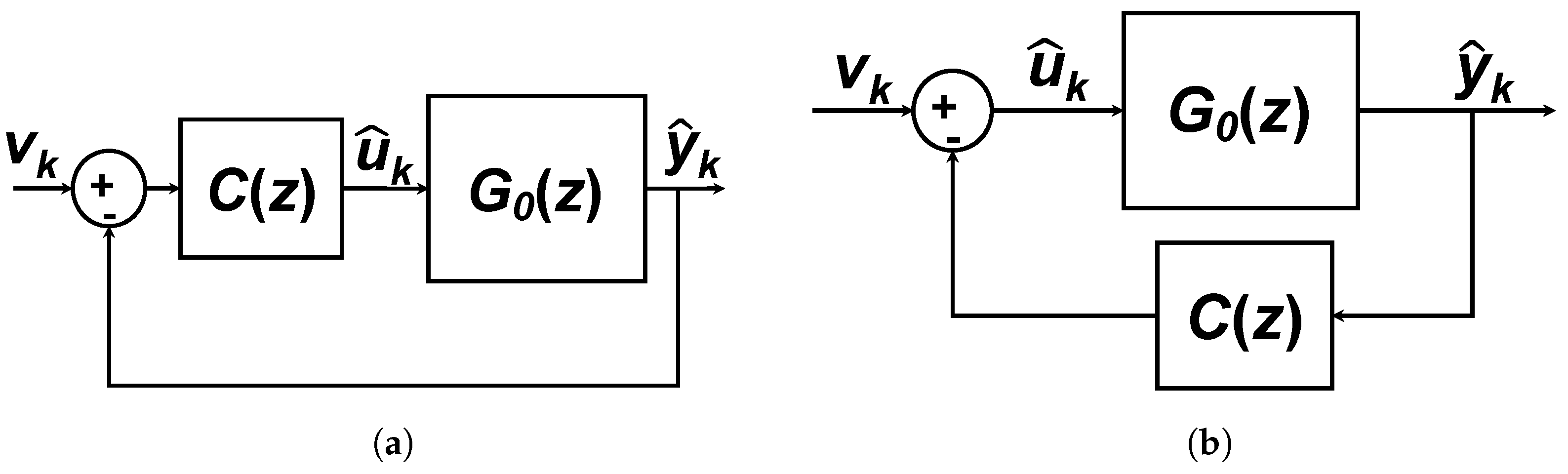
2.1. Pre-Compensating the Prediction Model

In order to obtain stable and well-damped output predictions, the model $G_0\left(z\right)$ in (1) is compensated using a bi-proper feedback controller $C\left(z\right)$, as shown in Figure 1a (or Figure 1b; see Remark 1). Note the following:

$$C\left(z\right)={\displaystyle \frac{q\left(z\right)}{p\left(z\right)}}$$

(2)

where $p\left(z\right)=1+p_1{z}^{-1}+\cdots +p_m{z}^{-m}$ and $q\left(z\right)=q_0+q_1{z}^{-1}+\cdots +q_m{z}^{-m}$. The resulting pre-stabilised delay-free prediction model is then given as follows:

$$G_{s,0}\left(z\right)={\displaystyle \frac{{\widehat{y}}_k}{v_k}}={\displaystyle \frac{q\left(z\right)b\left(z\right)}{p\left(z\right)a\left(z\right)+q\left(z\right)b\left(z\right)}}={\displaystyle \frac{\beta \left(z\right)}{\alpha \left(z\right)}}$$

(3)

where $v_k$ is the transformed decision variable which is computed via PFC, as shown in Figure 2. Hence, the i-step ahead output predictions can be obtained (see [12,19] for details) recursively from (3), i.e., $\alpha \left(z\right)\widehat{y}\left(z\right)=\beta \left(z\right)v\left(z\right)$ such that:

$$y_{k+i+n_d|k}={\mathbf{H}}_i{\underrightarrow{\mathbf{v}}}_k+{\mathbf{P}}_i{\underleftarrow{\mathbf{v}}}_{k-1}+{\mathbf{Q}}_i{\underleftarrow{\widehat{\mathbf{y}}}}_k+d_k$$

(4)

where $d_k=y_k-{\widehat{y}}_{k-nd}$ is added to remove prediction bias due to disturbance and/or uncertainties, and ${\mathbf{H}}_i$, ${\mathbf{P}}_i$, and ${\mathbf{Q}}_i$ depend on the model parameters $\alpha \left(z\right)$ and $\beta \left(z\right)$. Furthermore,

$${\underrightarrow{\mathbf{v}}}_k=\left[\begin{array}{c}{v}_k\\ v_{k+1}\\ ⋮\\ v_{k+i-1}\end{array}\right];{\underleftarrow{\mathbf{v}}}_{k-1}=\left[\begin{array}{c}{v}_{k-1}\\ v_{k-2}\\ ⋮\\ v_{k-l}\end{array}\right];{\underleftarrow{\widehat{\mathbf{y}}}}_k=\left[\begin{array}{c}{\widehat{y}}_k\\ {\widehat{y}}_{k-1}\\ ⋮\\ {\widehat{y}}_{k-l+1}\end{array}\right]$$

(5)

where $l=n+m$.

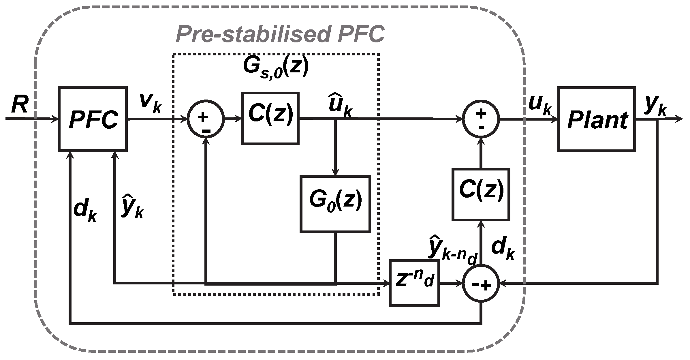
2.2. Establishing a Pre-Stabilised PFC Control Law

For simplicity, it is assumed that the output $y_k$ approaches the set-point R monotonically, i.e., exhibiting an ideal exponential trajectory. Thus, the desired i-step ahead tracking error can be expressed as follows:

$${\overline{e}}_{k+i+n_d|k}=(R-E\left[y_{k+n_d|k}\right]){\rho }^i;i\ge 1$$

(6)

where $\rho$ is the target pole $(0<\rho <1)$ representing the desired error reduction rate and $E\left[y_{k+n_d|k}\right]={\widehat{y}}_k+d_k$ is the expected delayed output. One may also obtain the actual error convergence using the output predictions (4):

$$e_{k+i+n_d|k}=R-\left({\mathbf{H}}_i{\underrightarrow{\mathbf{v}}}_k+{\mathbf{P}}_i{\underleftarrow{\mathbf{v}}}_{k-1}+{\mathbf{Q}}_i{\underleftarrow{\widehat{\mathbf{y}}}}_k+d_k\right);i\ge 1$$

(7)

Keeping $v_k$ constant, i.e., $v_{k+i}=v_k$, $\forall i\ge 1$, the desired and true errors, in (6) and (7) above, are matched at only one future instant $n_y$, known as the coincidence point, such that ${\overline{e}}_{k+n_y+n_d|k}=e_{k+n_y+n_d|k}$. Enforcing this coincidence defines the corresponding Pre-stabilised PFC control law as follows:

$$v_k={\displaystyle \frac{1}{h_{n_y}}}\left[R-(R-E\left[y_{k+n_d|k}\right]){\rho }^{n_y}-({\mathbf{P}}_{n_y}{\underleftarrow{\mathbf{v}}}_{k-1}+{\mathbf{Q}}_{n_y}{\underleftarrow{\widehat{\mathbf{y}}}}_k+d_k)\right]$$

(8)

where $h_{n_y}={\mathbf{H}}_{n_y}{\mathbf{L}}_{n_y}$ with ${\mathbf{L}}_{n_y}={[11\dots 1]}_{1\times n_y}^T$.

2.3. Computing the True Process Input

As shown in Figure 2, the actual process input $u_k$ is related to $v_k$ indirectly via the model input ${\widehat{u}}_k$, where $u_k={\widehat{u}}_k$ only in the absence of uncertainties, i.e., when $d_k=0$ (see [19] for a complete derivation). Here, we state the final result:

$$u_k=B_0{v}_k+f_k;f_k=-\mathbf{A}{\underleftarrow{\mathbf{u}}}_{k-1}+\mathbf{B}{\underleftarrow{\mathbf{v}}}_{k-1}+\mathbf{E}{\underleftarrow{\mathbf{d}}}_k$$

(9)

where $\mathbf{A}$, $\mathbf{B}$, and $\mathbf{E}$ are obtained from the parameters $a\left(z\right)$, $\alpha \left(z\right)$, $p\left(z\right)$, and $q\left(z\right)$ as follows:

$$\begin{array}{cc}\hfill A\left(z\right)& =\alpha \left(z\right)p\left(z\right)=1+A_1{z}^{-1}+A_2{z}^{-2}+\dots \hfill \\ \hfill B\left(z\right)& =q\left(z\right)a\left(z\right)p\left(z\right)=B_0+B_1{z}^{-1}+B_2{z}^{-2}+\dots \hfill \\ \hfill E\left(z\right)& =-\alpha \left(z\right)q\left(z\right)=E_0+E_1{z}^{-1}+E_2{z}^{-2}+\dots \hfill \end{array}$$

(10)

Evidently, after pre-stabilisation, the degree-of-freedom (d.o.f.) is reparametrised appropriately, given a suitable inner controller $C\left(z\right)$, which can now work well, notwithstanding any difficult open-loop dynamics.

Remark 1.

If $C\left(z\right)$ is positioned in the feedback path of the pre-compensation loop, as shown in Figure 1b, rather than the forward path, the numerator of the pre-stabilised model $G_{s,0}\left(z\right)$ in (3) changes to $\beta \left(z\right)=p\left(z\right)b\left(z\right)$. Hence, the computation of $B\left(z\right)$ in (10) must also be updated accordingly with $B\left(z\right)=p\left(z\right)a\left(z\right)p\left(z\right)$. In this case, the coefficient $B_0$ will be equal to 1 as both $p\left(z\right)$ and $a\left(z\right)$ are monic polynomials.

2.4. Constraint Handling with Pre-Stabilisation

Although reparametrising the predicted input $u_k$ slightly complicates the computation, it is still possible to incorporate constraint handling into Pre-stabilised PFC in a systematic way, and while retaining nominal feasibility, as demonstrated in several recent papers [19]. In practice, it is sufficient to check the following inequalities up to a long enough validation horizon $n_c$, where $n_c>>n_y$

$$\begin{array}{cc}\hfill {\mathbf{L}}_{n_c}\underset{¯}{u}& \le {\underrightarrow{\mathbf{u}}}_k\le {\mathbf{L}}_{n_c}\overline{u}\hfill \\ \hfill {\mathbf{L}}_{n_c}\Delta \underset{¯}{u}& \le \Delta {\underrightarrow{\mathbf{u}}}_k\le {\mathbf{L}}_{n_c}\Delta \overline{u}\hfill \\ \hfill {\mathbf{L}}_{n_c}\underset{¯}{y}& \le {\underrightarrow{\mathbf{y}}}_{k+1}\le {\mathbf{L}}_{n_c}\overline{y}\hfill \end{array}$$

(11)

However, as these details are not central to the contribution of this paper, they are excluded for clarity.

2.5. Summary

In short, assuming the availability of a suitable inner-loop compensator, pre-stabilisation ensures smooth, well-damped, and monotonically convergent prediction dynamics. Nevertheless, the consequent reparametrisation of the predicted input, as given in (9), also complicates to some extent the simplistic constraint management offered by the conventional PFC algorithm, although given the modern computing capacity, this is not likely to be a problem.

3. Pre-Stabilised PFC and Relative Tuning

The primary tuning parameter $\rho$ in the control law (8) is central to achieving the desired time response; nonetheless, its efficacy [13] is highly dependent on the judicious selection of the coincidence point $n_y$. For example, if $n_y$ is chosen closer to the system’s steady state, the effect of $\rho$ diminishes as ${\rho }^{n_y}\to 0$. On the other hand, imposing coincidence early in the transient region may cause significant over-actuation. Furthermore, the inconsistent use of target/disturbance information in (8) may also cause additional lag in the response, which further weakens the desired link between the selected parameters and the achieved performance. Consequently, the conventional PFC often fails to fulfil the control objectives as per the desired specification [22].

To overcome these tuning deficiencies, this section examines a conceptually new approach to PFC tuning using relative statements, such as faster or slower with respect to the steady-state benchmark, as opposed to finding $\rho$ and $n_y$ on absolute terms.

3.1. The Relative Tuning Proposal

Assuming zero initial conditions and no uncertainty for simplicity, it is straightforward to show using (8) that for a change in R,

$$v_k={\displaystyle \frac{R}{h_{n_y}}}(1-{\rho }^{n_y})$$

(12)

Moreover, the steady-state control in nominal conditions may be computed as follows:

$$v_{ss}={\displaystyle \frac{R}{G_{s,0}\left(1\right)}};\because y_{ss}=R$$

(13)

where $G_{s,0}\left(1\right)$ is the steady-state gain of the pre-stabilised system, given by the following:

$$G_{s,0}\left(1\right)={\displaystyle \frac{\beta \left(1\right)}{\alpha \left(1\right)}}={\displaystyle \frac{{\beta }_1+{\beta }_2+\cdots +{\beta }_l}{1+{\alpha }_1+{\alpha }_2+\cdots +{\alpha }_l}}={\displaystyle \frac{{\sum }_{i=1}^l{\beta }_i}{1+{\sum }_{i=1}^l{\alpha }_i}}$$

(14)

Now, define a new tuning parameter $\theta$, the transient input aggression factor, as the ratio of the input $v_k$ to the steady-state input $v_{ss}$, that is,

$$\theta ={\displaystyle \frac{v_k}{v_{ss}}}={\displaystyle \frac{G_{s,0}\left(1\right)}{h_{n_y}}}(1-{\rho }^{n_y})$$

(15)

from which it is obvious whether one uses the left-hand side with $\theta$ or the right-hand side with $(\rho ,n_y)$, the relationship in (15) will tune the controller by suitably adjusting $v_k$ with respect to the steady-state input $v_{ss}$. Although both methods attempt to fulfil the same performance specification, using $\theta$ directly as the sole tuning parameter appears more efficient and transparent than the conventional methods of selecting $\rho$ and $n_y$ [2,12,13].

Hence, the proposed relative tuning can benefit in the following ways:

(i)

The controller tuning simplifies to merely answering one trivial question, i.e., how much faster (or slower) one wishes the closed-loop system to respond as compared to the open-loop behaviour.

(ii)

Removing the explicit role of $\rho$ and $n_y$ implicit in conventional PFC laws [22] prevents the incorrect use of feedforward information in the control law, and consequently the inadvertent addition of undesirable lag in the closed-loop response.

This, however, requires reformulating the control law, which is presented in the following sections.

Remark 2.

It is emphasised that the true estimate of the expected steady-state input must incorporate the error correction term $d_k$ to ensure bias-free tracking, which is necessary to accommodate the effect of modelling uncertainty and/or disturbance. Thus, the following corrected expression of $v_{ss}$ will be employed in the following derivation, as well as the simulation studies presented in Section 5 of this article:

$$E\left[v_{ss}\right]={\displaystyle \frac{R-d_k}{G_{s,0}\left(1\right)}}$$

(16)

3.2. The Relative PFC Control Law

Just like the conventional PFC, the proposed Relative PFC also relies on three key elements: a suitable prediction model, a benchmark response, and a mechanism to ensure bias-free predictions. Nevertheless, instead of using an ideal exponential trajectory and the concept of coincidence, the system’s response to the steady-state input is utilised as a benchmark for the closed-loop performance tuning.

With $v_k=v_{ss}$, the following $n_y$-step ahead predicted error convergence is obtained:

$${\overline{e}}_{k+n_y+n_d|k}=R-(h_{n_y}{v}_{ss}+{\mathbf{P}}_{n_y}{\underleftarrow{\mathbf{v}}}_{k-1}+{\mathbf{Q}}_{n_y}{\underleftarrow{\widehat{\mathbf{y}}}}_k+d_k);$$

(17)

which compares to (7) with $i=n_y$ (here, $n_y$ represents the length of the prediction horizon). Thus, to ensure a faster convergence than the benchmark (17), one must select a $v_k$ correspondingly more active than $v_{ss}$. Lemma 1 below formalises this concept.

Lemma 1.

In the nominal state and zero initial conditions, the choice $v_k=\theta v_{ss}$ for the target R provides an error convergence which is γ times (17) when

$$\gamma ={\displaystyle \frac{G_{s,0}\left(1\right)-h_{n_y}\theta }{G_{s,0}\left(1\right)-h_{n_y}}}$$

(18)

Proof. 

With $d_k$, ${\underleftarrow{\mathbf{v}}}_{k-1}$ and ${\underleftarrow{\widehat{\mathbf{y}}}}_k$ all zero, and $v_k=\theta v_{ss}$, the tracking errors are related as follows:

$$R-h_{n_y}\theta v_{ss}=\gamma (R-h_{n_y}{v}_{ss})$$

using (13) then implies

$$1-{\displaystyle \frac{h_{n_y}\theta }{G_{s,0}\left(1\right)}}=\gamma \left(1-{\displaystyle \frac{h_{n_y}}{G_{s,0}\left(1\right)}}\right)$$

which simplifies to (18) after simple manipulations. □

Theorem 1.

For the chosen input activity θ and the error convergence γ defined in (18) above, the pre-stabilised relative PFC (PRPFC) control law is given as follows:

$$v_k=\gamma v_{ss}+{\displaystyle \frac{1-\gamma }{h_{n_y}}}\left[R-\left({\mathbf{P}}_{n_y}{\underleftarrow{\mathbf{v}}}_{k-1}+{\mathbf{Q}}_{n_y}{\underleftarrow{\widehat{\mathbf{y}}}}_k+d_k\right)\right]$$

(19)

Proof. 

Using Lemma 1, it is clear that $e_{k+n_y+n_d|k}=\gamma {\overline{e}}_{k+n_y+n_d|k}$, implying the following:

$$R-(h_{n_y}{v}_k+{\mathbf{P}}_{n_y}{\underleftarrow{\mathbf{v}}}_{k-1}+{\mathbf{Q}}_{n_y}{\underleftarrow{\widehat{\mathbf{y}}}}_k+d_k)=\gamma \left[R-(h_{n_y}{v}_{ss}+{\mathbf{P}}_{n_y}{\underleftarrow{\mathbf{v}}}_{k-1}+{\mathbf{Q}}_{n_y}{\underleftarrow{\widehat{\mathbf{y}}}}_k+d_k)\right]$$

which simplifies to the control law (19). □

Note that the true process input $u_k$ can be easily computed using (9) as before.

3.3. Parameter Tuning in RPFC

The core benefit of relative PFC is obvious from the preceding discussion, as the closed-loop performance tuning now reduces to simply answering one statement: how fast or slow does one want the closed-loop system to respond as compared to the benchmark behaviour based on steady-state inputs? More specifically, the proposal provides three distinct tuning choices, i.e., $0<\theta <1$, $\theta =1$, and $\theta >1$, each with the following interpretation:

• $0<\theta <1$ reduces the input activity, resulting in a slower closed-loop performance. For example, $\theta =0.5$ uses an input only half as active as the benchmark to produce a relatively slower response.
• $\theta =1$ is equivalent to the steady-state tuning.
• $\theta >1$ increases input activity with a faster performance. For example, $\theta =2$ uses an input twice as aggressive as the benchmark to produce a comparatively faster response.

Remark 3.

It is advised to practice caution while selecting θ, as large values may over-actuate the controller. Clearly, a more sensible approach would be to keep the actuating capacity of the system under consideration while making the ultimate tuning selection.

3.4. Managing Constraints with Pre-Stabilised Relative PFC

In addition to significant tuning simplifications, another benefit of the proposal is that it does not modify or complicate the process of handling constraints any further, which may be performed as discussed earlier in Section 2.4 of this paper.

3.5. Summary

The core conceptual novelty of this section is the introduction to relative tuning within a dual-loop setting. This is simple, intuitive, and far more transparent than the conventional tuning approaches adopted in PFC or even PID controllers. The obvious requirement here is the availability of system dynamics that are broadly acceptable, i.e., ideally well-damped, stable, and monotonically convergent to the steady state. Thus, in difficult applications where this is not the case, the dual-loop control strategy presented earlier can be implemented to benefit from simplified tuning offered by relative PFC.

4. Designing a Suitable Pre-Stabilising Compensator

In this section, we present a selection of four recently proposed pre-stabilisation schemes that are simple, well-understood, and easily implementable with basic technical know-how and, more importantly, without overly complicating the PFC design [19,20,24,25]. Note, as will be evident in the following subsections, the use of these strategies has been classified according to the type of dynamics, i.e., first-, second-, or more generic higher-order, for which they are designed.

4.1. Pre-Compensation of Unstable First-Order Dynamics

Consider an unstable first-order system given as follows [24]:

$$G_0\left(z\right)={\displaystyle \frac{b_1{z}^{-1}}{1-a_1{z}^{-1}}};a_1\ge 1$$

(20)

This system can be easily stabilised with a simple proportional gain $C\left(z\right)=K$ as per the proposed configuration shown in Figure 1a. The resulting pre-stabilised system has the following transfer function:

$$G_{s,0}\left(z\right)={\displaystyle \frac{{\beta }_1{z}^{-1}}{1-{\alpha }_1{z}^{-1}}}={\displaystyle \frac{K{b}_1{z}^{-1}}{1-(a_1-K{b}_1)z^{-1}}}$$

(21)

Theorem 2.

The compensated predictions in (21) are stable and monotonically convergent provided K is selected within the following range:

$${\displaystyle \frac{1-a_1}{b_1}}<K<-{\displaystyle \frac{a_1}{b_1}}$$

(22)

Proof. 

For convergent predictions, the pre-stabilised pole ${\alpha }_1$ must be stable, i.e., must lie within the range $0<{\alpha }_1<1$, implying the following:

$$0<a_1-K{b}_1<1$$

which after simple manipulations leads to (22). □

Although Theorem 2 in principle defines the upper and lower bounds on K for guaranteed stability, a more systematic choice of the pre-stabilised pole is ${\alpha }_1=1/a_1$ (if $a_1>1$), which means the pre-stabilising compensator may be designed by selecting the following:

$$K={\displaystyle \frac{a_1^2-1}{a_1{b}_1}}$$

(23)

In case the open-loop system exhibits integrator dynamics, i.e., $a_1=1$, then one may simply select ${\alpha }_1=0.5$ by choosing $K=0.5/b_1$. This pre-stabilises $G_0\left(z\right)$ in a straightforward manner.

4.2. Pre-Stabilising Second-Order Dynamics via Root Locus

This proposal (see [25]) is fairly generic and is based on the fact that a majority of real-world processes can be adequately represented as dominant second-order dynamics, for which simple tailored solutions are well understood.

Assume that a simple proportional controller, i.e., $C\left(z\right)=K$, is utilised in the feedback path of the inner loop, as shown in Figure 1b, to compensate a difficult second-order system $G_0\left(z\right)$, resulting in the following pre-stabilised transfer function:

$$G_{s,0}\left(z\right)={\displaystyle \frac{\beta \left(z\right)}{\alpha \left(z\right)}}={\displaystyle \frac{G_0\left(z\right)}{1+K{G}_0\left(z\right)}}={\displaystyle \frac{b\left(z\right)}{a\left(z\right)+Kb\left(z\right)}}$$

(24)

where $a\left(z\right)=1+a_1{z}^{-1}+a_2{z}^{-2}$ and $b\left(z\right)=b_1{z}^{-1}+b_2{z}^{-2}$. A simple approach is to design the proportional gain K via Root Locus, which is a powerful graphical tool for control systems’ analysis and design [26]. Hence, one may analyse the effect of K on the pre-stabilised pole polynomial $\alpha \left(z\right)$, with the goal to obtain critically (or, in practice, close to) damped poles at the stable break-in/breakaway points, denoted by $\sigma$, on the root loci, as shown in Figure 3. Consequently, at $z=\sigma$, the compensator K must satisfy the following gain condition [27]:

$$K\left(\sigma \right)=-{\displaystyle \frac{1}{G_0\left(\sigma \right)}}=-{\displaystyle \frac{a\left(\sigma \right)}{b\left(\sigma \right)}}$$

(25)

where the function $K\left(\sigma \right)$ demonstrates the local minimum/maximum at the break-in/breakaway points. Thus, being stationary, these points can be obtained analytically by taking the first derivative of (25) with respect to $\sigma$:

$${\displaystyle \frac{dK\left(\sigma \right)}{d\sigma }}=-{\displaystyle \frac{d}{d\sigma }}\left[{\displaystyle \frac{a\left(\sigma \right)}{b\left(\sigma \right)}}\right]=0$$

In practice, one could use computer tools to solve for $K\left(\sigma \right)$ quite quickly, but for second-order systems, simple analytic solutions exist, for example,

$${\sigma }_i=-{\displaystyle \frac{b_2}{b_1}}\pm {\displaystyle \frac{1}{b_1}}\sqrt{a_2{b_1}^2-a_1{b}_1{b}_2+{b_2}^2},i=1,2$$

(26)

Depending on the open-loop model parameters, two values of $\sigma$ are obtained from (26), but only the one within the range $0<\sigma <1$ can be implemented for pre-stabilisation. Hence, the pre-stabilised pole polynomial $\alpha \left(z\right)$ must be equal to $\alpha \left(z\right)=z^2-2\sigma z+{\sigma }^2$ with K evaluated from (25). It is also reiterated that one can easily find K using modern software tools and thus avoid explicit use of the algebra above.

Remark 4.

The open-loop zero dynamics of $G_0\left(z\right)$ may be significant in some instances, i.e., the root of $b\left(z\right)$ may appear in the vicinity of the system poles, hindering the successful implementation of this approach. In such cases, it is recommended to design a lead or lag type controller if possible to cancel and replace the problematic zero in order to minimise its undesirable effect. Interested readers are referred to [25] for details.

4.3. Pre-Compensation of Poorly Damped Systems via Pole Cancellation

Assume that $G_0\left(z\right)$ represents a nth-order under-damped, i.e., oscillatory, but otherwise stable system, such that [20]

$$G_0\left(z\right)={\displaystyle \frac{b\left(z\right)}{a\left(z\right)}};a\left(z\right)=a^{-}\left(z\right)a^{+}\left(z\right)$$

(27)

where $a^{+}\left(z\right)$ represents $p_u$ complex conjugate poles and $a^{-}\left(z\right)$ factors the remaining $n-p_u$ well-damped open-loop poles. As shown in Figure 1a, the cascade compensation of $G_0\left(z\right)$ with $C\left(z\right)$ results in the following pre-stabilised transfer function:

$$G_{s,0}\left(z\right)={\displaystyle \frac{\beta \left(z\right)}{\alpha \left(z\right)}}={\displaystyle \frac{C\left(z\right)G_0\left(z\right)}{1+C\left(z\right)G_0\left(z\right)}}$$

(28)

which after simple manipulations leads to the following:

$$C\left(z\right)={\displaystyle \frac{\beta \left(z\right)a\left(z\right)}{b\left(z\right)\left[\alpha \right(z)-\beta (z\left)\right]}}$$

(29)

Evidently, the open-loop zeros $b\left(z\right)$ become compensator poles that could possibly destabilise the system due to non-minimum phase dynamics. To avoid this issue, we set $\beta \left(z\right)=Kb\left(z\right)$ with $K\ne 0$ and therefore obtained the following:

$$C\left(z\right)=K{\displaystyle \frac{a\left(z\right)}{\alpha \left(z\right)-Kb\left(z\right)}}$$

(30)

where K can be evaluated easily, for example, via Root Locus. Hence, this compensator actually cancels the open-loop poles $a\left(z\right)$ and places the new poles defined by the polynomial $\alpha \left(z\right)$, which means it is necessary to select the pre-stabilised pole polynomial first before designing $C\left(z\right)$. Ideally, one would want the compensated model to exhibit non-oscillatory behaviour, for which a good starting point is to place the new poles of $G_{s,0}\left(z\right)$ at the projection of the dominant oscillatory poles of $G_0\left(z\right)$ along the real axis on the z-plane. The resulting pre-stabilised transfer function has the following form:

$$G_{s,0}\left(z\right)=K{\displaystyle \frac{b\left(z\right)}{\alpha \left(z\right)}};\alpha \left(z\right)=a^{-}\left(z\right){\alpha }^{+}\left(z\right)$$

(31)

where ${\alpha }^{+}\left(z\right)$ represents the $p_u$ pre-stabilised poles, such that ${\alpha }^{+}\left(z\right)={\prod }_{i=1}^{p_u}\left[z-\Re \left(z_{p,i}\right)\right]$ for each open-loop complex conjugate pole $z_{p,i}$ present in $a^{+}\left(z\right)$.

It is worth emphasising that despite being simple and intuitive, this method is not suitable for stabilising open-loop unstable systems due to the explicit pole cancellation in the control law [20].

4.4. Pre-Stabilisation via Pole Placement

Assume that a $(n-1)$th-order bi-proper compensator $C\left(z\right)$ is used to modify the open-loop model $G_0\left(z\right)$, as shown in Figure 1a, resulting in the pre-stabilised transfer function $G_{s,0}\left(z\right)$, with a smooth and monotonically convergent prediction behaviour. Then, the resulting ${(2n-1)}^{th}$-order pole polynomial $\alpha \left(z\right)$ is given by the following relationship [19]:

$$p\left(z\right)a\left(z\right)+q\left(z\right)b\left(z\right)=\alpha \left(z\right)$$

(32)

which is commonly known as the Diophantine Equation. In order to design $C\left(z\right)$, one must define the desired pre-stabilised characteristic polynomial $\alpha \left(z\right)$ and then utilise linear algebra to obtain the coefficients of $p\left(z\right)$ and $q\left(z\right)$ as follows:

$$\mathbf{M}={\mathbf{S}}^{-1}\mathbf{D}$$

(33)

where $\mathbf{M}={[p_{n-1}\dots 1q_{n-1}\dots q_0]}^T$, $\mathbf{D}={[{\alpha }_{2n-1}\dots {\alpha }_0]}^T$, and $\mathbf{S}$ is the Sylvester Matrix [28] given as follows:

$$\mathbf{S}=\left[\begin{array}{cccccccc}{a}_n& 0& \dots & 0& b_n& 0& \dots & 0\\ a_{n-1}& a_n& \dots & 0& b_{n-1}& b_n& \dots & 0\\ ⋮& ⋮& \dots & ⋮& ⋮& ⋮& \dots & ⋮\\ 1& a_1& \dots & a_{n-1}& 0& b_1& \dots & b_{n-1}\\ 0& 1& \dots & a_{n-2}& 0& 0& \dots & b_{n-2}\\ ⋮& ⋮& \dots & ⋮& ⋮& ⋮& \dots & ⋮\\ 0& 0& \dots & a_1& 0& 0& \dots & b_1\\ 0& 0& \dots & 1& 0& 0& \dots & 0\end{array}\right]$$

(34)

Note that $\alpha \left(z\right)$ is factorised as follows:

$$\alpha \left(z\right)=o\left(z\right)a^{-}\left(z\right){\alpha }^{+}\left(z\right)$$

(35)

where $o\left(z\right)$ is the $(n-1)$th-order observer, generally selected as $o\left(z\right)=z^{n-1}$, $a^{-}\left(z\right)$ factors the stable open-loop poles, and ${\alpha }^{+}\left(z\right)$ represents the $p_u$ pre-stabilised poles. If $a^{+}\left(z\right)={\prod }_{i=1}^{p_u}(z-z_{p,i})$, then the following is true.

• Proposal for Unstable Poles. With $z_{p,i}>1$, design ${\alpha }^{+}\left(z\right)={\prod }_{i=1}^{p_u}(z-1/z_{p,i})$. In case an integrator factor $(z-1)$ is present, one may simply replace it with $(z-0.5)$.
• Proposal for Complex Poles. With $z_{p,i}\in \mathbb{C}$, place the pre-stabilised poles at the real part of the complex open-loop poles, i.e., ${\alpha }^{+}\left(z\right)={\prod }_{i=1}^{p_u}\left(z-\Re \left(z_{p,i}\right)\right)$. This will effectively filter out the undesirable oscillations but without changing the convergence speed.

4.5. Summary

This section has presented a selection of classical feedback control techniques that integrate systematically into the dual-loop PFC framework. Though there are many choices available for a particular system at hand, ideally one should try the simplest controllers first, i.e., those based on proportional or proportional plus derivative elements, before opting for more complex higher-order designs based on, for example, pole cancellation or pole placement. This is important because a simpler inner loop naturally implies computationally efficient closed-loop constraint handling as well as simple coding and maintenance, akin to the original PFC algorithm, despite the added complexity of pre-compensation.

5. Simulation Results and Discussion

In this section, we investigate, compare, and contrast the closed-loop performance achieved with the proposed dual-loop control strategy. To highlight the benefits of the approach, the analysis also includes a comparison with the Conventional PFC (CPFC) and PID control algorithms in real world scenarios, i.e., in the presence of process constraints, disturbances, measurement noise, and modelling mismatches.

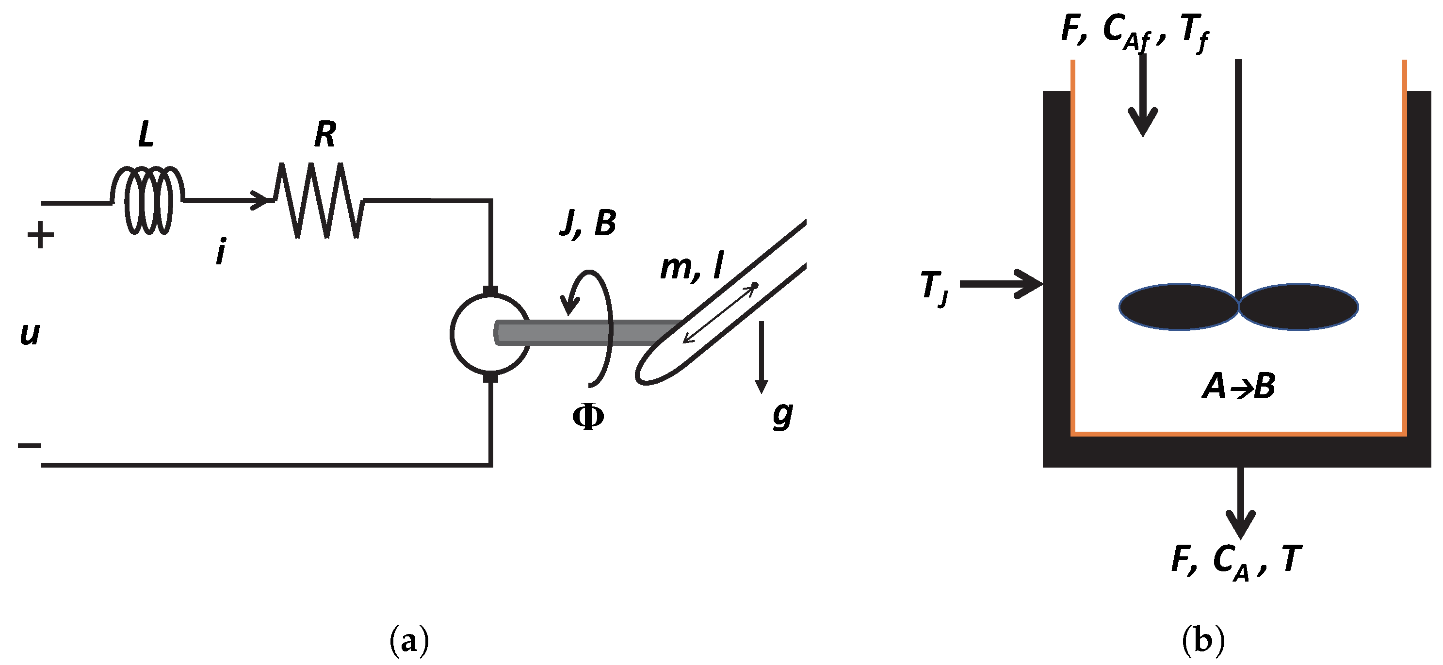
5.1. Description of Case Studies

Let us begin by introducing the two challenging open-loop industrial processes that will be used as case studies in the following sections.

Position Control of Single Link Robotic Arm. Robotic manipulators have played a vital role in global industrialisation, leading to better-quality products with cheaper manufacturing costs. This study implements the dual-loop relative PFC algorithm to control the angular position of a single-link robotic arm driven by a brushed DC motor, as shown in Figure 4a. The non-linear model of the manipulator has three coupled states, i.e., the angular position $\varphi$, the angular velocity $\dot{\varphi }$, and the motor current i, related to each other according to the following dynamic relationship [29]:

$$\begin{array}{cc}\hfill J{\displaystyle \frac{d^2\varphi }{d{t}^2}}+B{\displaystyle \frac{d\varphi }{dt}}+mglsin\varphi & =K_{\tau }i\hfill \end{array}$$

(36a)

$$\begin{array}{cc}\hfill L{\displaystyle \frac{di}{dt}}+Ri+K_e{\displaystyle \frac{d\varphi }{dt}}& =u\hfill \end{array}$$

(36b)

where u is the input voltage (manipulated variable), J is the inertia of the robotic arm, B represents the actuator damping, m and l denote the mass and length of the arm, g is acceleration due to gravity, L and R represent the inductance and resistance of the motor winding, $K_{\tau }$ is the torque constant, and $K_e$ represents the voltage constant of the motor. These parameters are assumed to have the following numerical values: $J=0.1$ kgm², $B=0.05$ Nms/rad, $m=2$ kg, $l=0.75$ m, $g=9.8$ m/s², $K_{\tau }=0.768$ Nm/A, $K_e=0.768$ Nms/rad, $R=2.6 \Omega$, and $L=25$ mH. Moreover, the motor voltage supply is limited between $0\le u\le 24$ volts with $|\Delta u|\le 0.5$ volts/s.

Temperature control in Jacketed CSTR. The Continuous Stirred Tank Reactor (CSTR) is a common industrial unit widely employed in different chemical manufacturing processes. In this study, we consider a specific type of CSTR equipped with an outer jacket in which the temperature of a flowing fluid $T_J$ is used to regulate the inside reaction temperature T, as shown in Figure 4b. The overall coupled model has two-state non-linear dynamics, as given below [30]:

$$\begin{array}{cc}\hfill {\displaystyle \frac{d{C}_A}{dt}}& ={\displaystyle \frac{F}{V}}\left(C_{A_f}-C_A\right)-k_0{e}^{-\frac{E}{R_{g}T}}{C}_A\hfill \end{array}$$

(37a)

$$\begin{array}{cc}\hfill {\displaystyle \frac{dT}{dt}}& ={\displaystyle \frac{F}{V}}\left(T_f-T\right)+\left({\displaystyle \frac{-\Delta H}{\rho C_p}}\right)k_0{e}^{-\frac{E}{R_{g}T}}{C}_A-{\displaystyle \frac{UA}{V\rho C_p}}\left(T-T_J\right)\hfill \end{array}$$

(37b)

where $C_A$ is the concentration of component A, T is the reaction temperature, $C_{A_f}$ is the feed concentration, $T_f$ is the feed temperature, $T_J$ is the jacket temperature, F is the input flow rate, V is the reactor volume, $k_0$ is the frequency factor, E is the activation energy, $R_g$ is the ideal gas constant, $-\Delta H$ is the heat of reaction, U is the heat transfer coefficient, A is the area of heat transfer, $\rho$ is the fluid density, and $C_p$ is the fluid heat capacity. The following parametric values have been used in simulations [31]: $k_0=16.96\times {10}^{12}$ h⁻¹, $E=\mathrm{32,400}$ Btu/lb mol, $R_g=1.987$ Btu/lb mol°F, $\rho C_p=53.25$ Btu/ft³°F, $UA=\mathrm{23,200}$ Btu/h°F, $V=500$ ft³, $F=2000$ ft³/h, $C_{A_f}=0.132$ lb mol/ft³, and $T_f=60$ °F. Furthermore, the jacket fluid temperature is limited to a maximum value, such that $T_J\le 2640$ °F.

5.2. Linearisation of Models

The single-link robotic arm (36) is linearised, using a sampling period of 10 ms, around the operating point ${\varphi }_{ss}=0.314$ rad (18°) and $u_{ss}=15.4$ volts, leading to the following:

$$G_1={\displaystyle \frac{{\varphi }^{\prime }\left(z\right)}{u^{\prime }\left(z\right)}}={\displaystyle \frac{4.011z^2+12.596z+2.384}{z^3-2.320z^2+1.681z-0.352}}\times {10}^{-5}$$

(38)

where ${\varphi }^{\prime }$ and $u^{\prime }$ are the output and input deviation variables around their corresponding steady-state values. A second-order model is also constructed using the model reducer app available in MATLAB 2021a [32]:

$$G_{1,r}={\displaystyle \frac{{\varphi }^{\prime }\left(z\right)}{u^{\prime }\left(z\right)}}={\displaystyle \frac{-1.192z+4.133}{z^2-1.962z+0.972}}\times {10}^{-2}$$

(39)

Note that both linear transfer function models (38) and (39) exhibit significant oscillations with open-loop poles positioned at $z=0.362,0.979\pm j0.117$ for $G_1$ and $z=0.981\pm j0.101$ for $G_{1,r}$.

Similarly, the jacketed CSTR process (37) is linearised using a sampling period of $0.01$ min ($0.6$ s) around the operating point $T_{ss}=560.8$ °F and $T_{J,ss}=2637.9$ °F, resulting in an unstable second-order dynamic model (assuming a measurement delay of $n_d=25$ samples) given as follows:

$$G_2={\displaystyle \frac{T^{\prime }\left(z\right)}{T_J^{\prime }\left(z\right)}}={\displaystyle \frac{0.00895z-0.00825}{z^2-1.972z+0.9719}}{z}^{-25}$$

(40)

where both $T^{\prime }$ and $T_J^{\prime }$ are deviation variables around the corresponding steady-state values. A first-order model is also constructed using the model reducer app available in MATLAB 2021a [32]:

$$G_{2,r}={\displaystyle \frac{T^{\prime }\left(z\right)}{T_J^{\prime }\left(z\right)}}={\displaystyle \frac{0.0205}{z-1.004}}{z}^{-25}$$

(41)

Note that both linear transfer function models (40) and (41) exhibit output instability with open-loop poles positioned at $z=0.969,1.004$ for $G_2$ and $z=1.004$ for $G_{2,r}$.

5.3. Pre-Stabilisation and Parameter Tuning

The third-order model $G_1$ (38) and the reduced second-order model $G_{1,r}$ (39) of the robotic arm were pre-stabilised using the Pole Placement (PP), Pole Cancellation (PC), and Root Locus (RL) methods. The associated pre-stabilising compensators, designed using the strategies discussed in Section 4, are as follows:

• $C_1^{PP}={\displaystyle \frac{-66.29z^2+18.2z+2.09}{z^2+0.00266z+0.00014}}$
• $C_1^{PC}={\displaystyle \frac{0.3z^3-0.696z^2+0.5042z-0.1055}{z^3-2.32z^2+1.67z-0.347}}$
• $C_{1,r}^{RL}=-32$

Consequently the following pre-compensated transfer function models were obtained:

• $G_1^{PP}={\displaystyle \frac{-265.90z^4-761.96z^3+79.55z^2+69.71z+4.98}{z^5-2.32z^4+1.67z^3-0.346z^2}}\times {10}^{-5}$
• $G_1^{PC}={\displaystyle \frac{1.20z^2+3.78z+0.715}{z^3-2.32z^2+1.67z-0.347}}\times {10}^{-5}$
• $G_{1,r}^{RL}={\displaystyle \frac{-15z+44.5}{z^2-1.96z+0.958}}\times {10}^{-5}$

The dominant pre-stabilised poles positioned at $z=$ 0.979, 0.979 in each case warrant an equivalent closed-loop behaviour in nominal conditions, which is indeed obvious from Figure 5a, depicting the benchmark (mean-level) system outputs with $\theta =1$. Furthermore, Figure 5b clearly indicates the tuning efficacy of the proposed pre-stabilised PFC algorithms, i.e., PPFC-PP, PPFC-PC, and PPFC-FO, with $\theta =5$, as the robotic arm now settles relatively quickly to its target steady-state angular position as compared to the benchmark responses shown in Figure 5a; the increase in the corresponding transient input magnitude is also clear.

In the unstable jacketed CSTR example, the original second-order model $G_2$ (40) along with its reduced first-order model $G_{2,r}$ (41) are pre-stabilised using the Pole Placement (PP), Root Locus (RL), and First-Order (FO) methods. Note that due to the presence of the open-loop unstable mode, the Pole Cancellation method was not utilised for pre-compensation.

• $C_2^{PP}={\displaystyle \frac{9.834z-9.525}{z-0.0808}}$, $G_2^{PP}={\displaystyle \frac{0.088z^2-0.166z+0.079}{z^3-1.965z^2+0.965z}}$, poles at $0,0.997,0.969$
• $C_2^{RL}=0.556$, $G_2^{RL}={\displaystyle \frac{0.00895z-0.00825}{z^2-1.967z+0.9673}}$, poles at $0.984,0.984$
• $C_{2,r}^{FO}=0.389$, $G_{2,r}^{FO}={\displaystyle \frac{0.00798}{z-0.996}}$, pole at $0.996$

The Root Locus method here provides relatively faster dominant poles than the other two techniques; hence, its pre-stabilised benchmark response (PPFC-RL) is correspondingly faster, as shown in Figure 6a. Nevertheless, the selected tuning parameter $\theta =3$ works effectively by producing relatively faster closed-loop outputs (Figure 6b). However, pre-compensation via pole placement in this case is likely not a good choice since the sharp initial input peak (for both $\theta =1,3$) is large compared to other methods; this could cause constraint violations and even worse lead to instability in consequence.

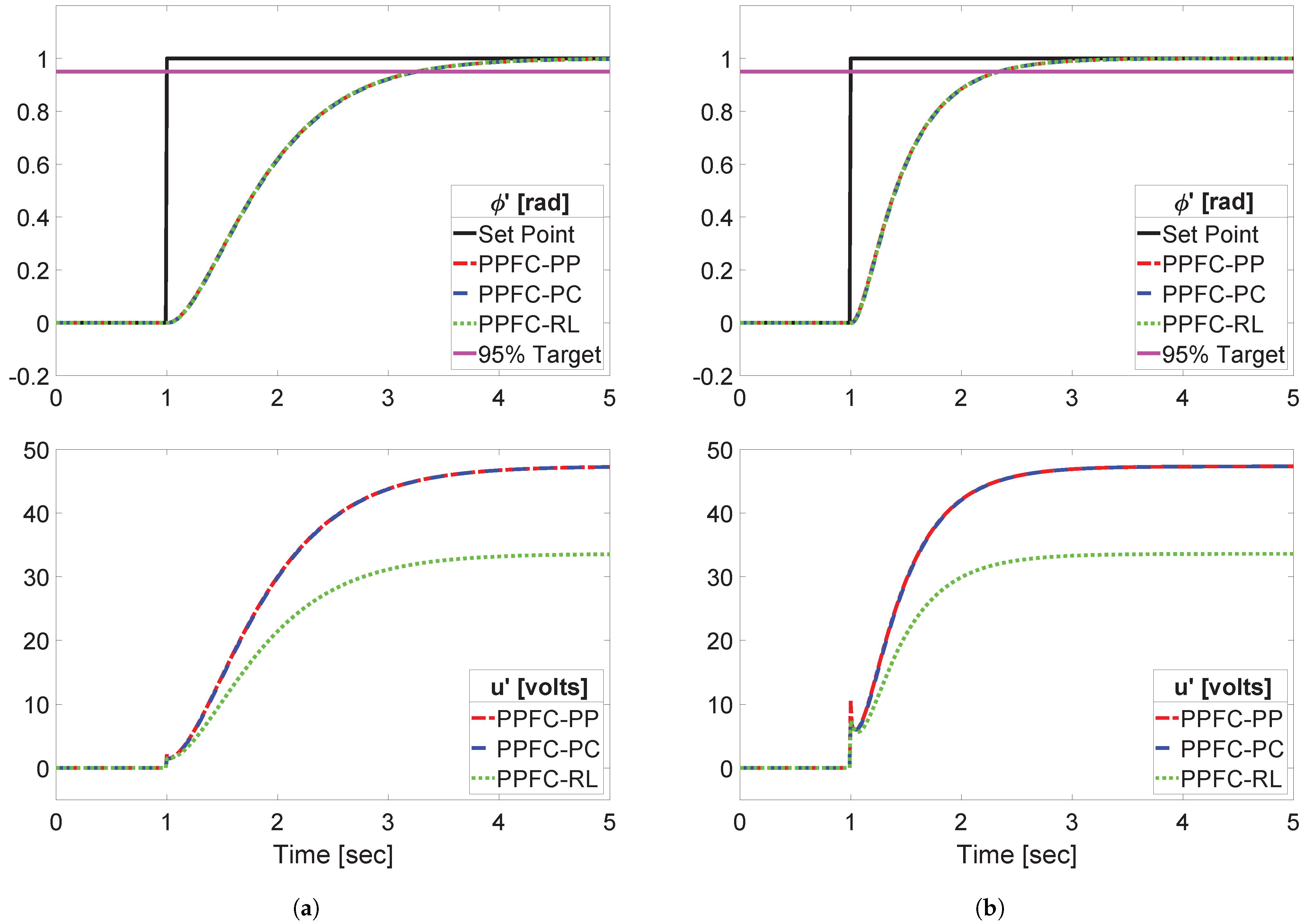
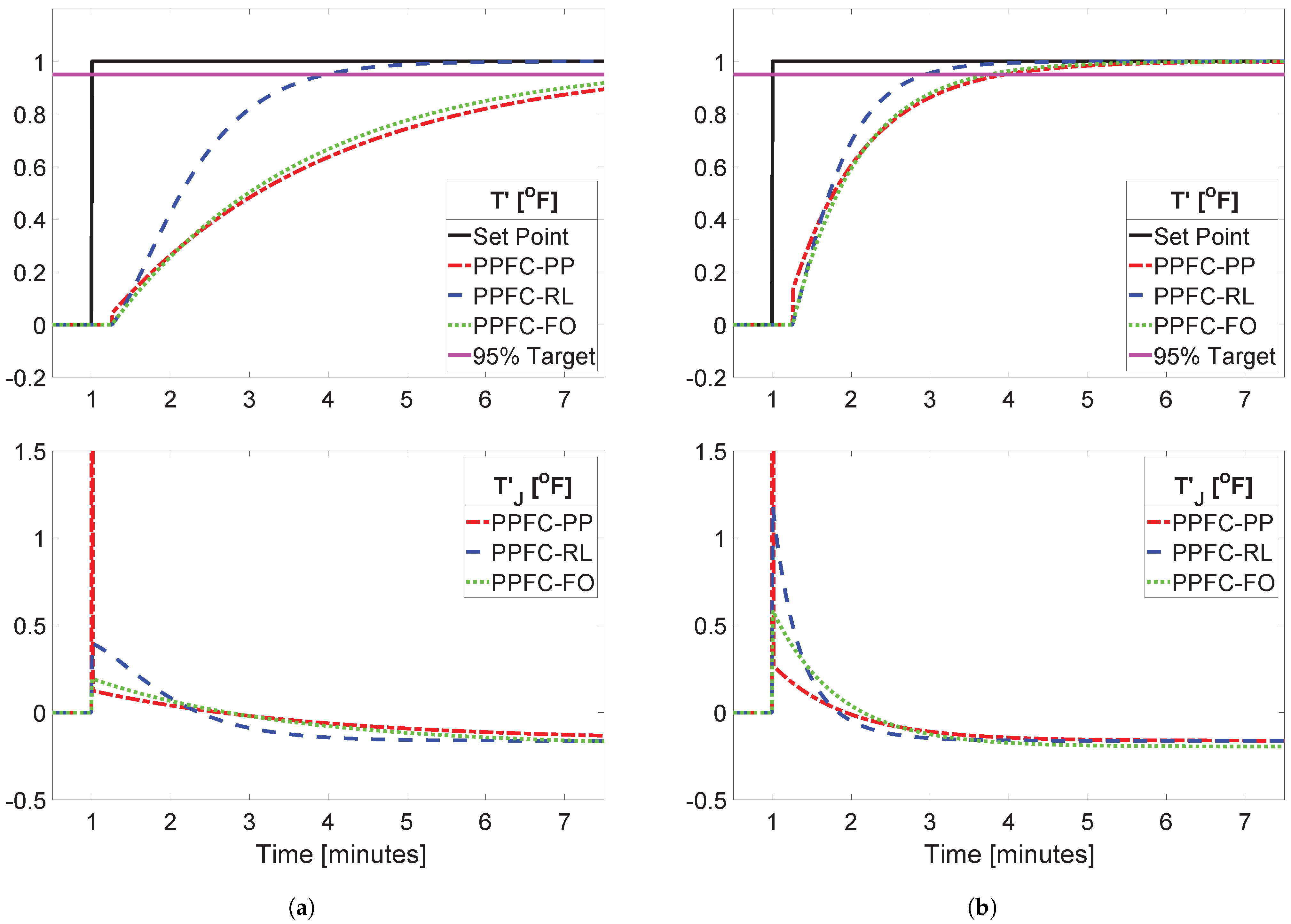
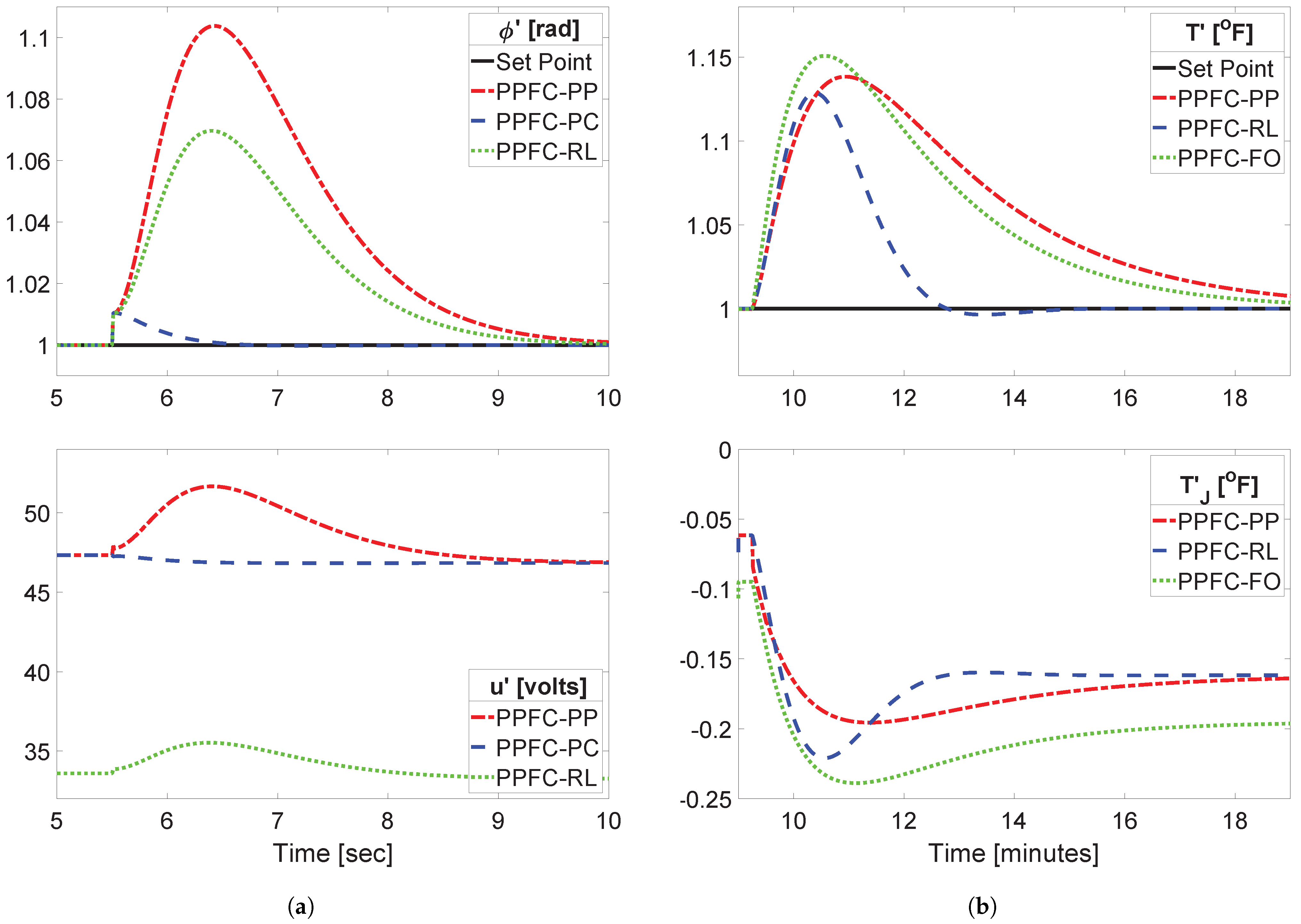
5.4. Comparison in Practical Scenarios

We further analysed the closed-loop performance of these pre-stabilisation methods in more practical scenarios by incorporating the effect of external disturbances, measurement noise, and modelling uncertainties.

For the single-link robot, a constant disturbance of 0.1 rad was introduced at the process output, whereas for the unstable CSTR, a constant input disturbance of 1 °F was added. The results are shown in Figure 7, from which it is evident that the Pole Placement method in both cases demonstrates relatively sluggish disturbance rejection as compared to the other two methods. Notably, Pole Cancellation provides by far the best performance, with significantly faster disturbance rejection and output normalisation. A similar trend is observed in the noise and uncertainty management (see Figure 8), which shows the PPFC-PP being far more adversely affected than any of the other methods, especially for the unstable process example.

Table 1. Comparison of Mean Absolute Error (MAE) for different pre-stabilisation techniques used in Section 5.3 and Section 5.4.

S. No.	Scenario	Case Study 1	Case Study 2
		$\theta =1$	$\theta =1$
		$MA{E}^{PP}=0.0384$	$MA{E}^{PP}=0.1166$
		$MA{E}^{PC}=0.0386$	$MA{E}^{RL}=0.0523$
		$MA{E}^{RL}=0.0383$	$MA{E}^{FO}=0.1082$
1.	No disturbance, noise, and/or modelling uncertainty	$\theta =5$	$\theta =3$
		$MA{E}^{PP}=0.0208$	$MA{E}^{PP}=0.0423$
		$MA{E}^{PC}=0.0210$	$MA{E}^{RL}=0.0342$
		$MA{E}^{RL}=0.0208$	$MA{E}^{FO}=0.0426$
		$\theta =5$	$\theta =3$
		$MA{E}^{PP}=0.0279$	$MA{E}^{PP}=0.0663$
2.	Added disturbance	$MA{E}^{PC}=0.0212$	$MA{E}^{RL}=0.0432$
		$MA{E}^{RL}=0.0254$	$MA{E}^{FO}=0.0645$
		$\theta =5$	$\theta =3$
		$MA{E}^{PP}=0.0428$	$MA{E}^{PP}=0.0490$
3.	Added measurement noise and modelling uncertainty	$MA{E}^{PC}=0.0320$	$MA{E}^{RL}=0.0421$
		$MA{E}^{RL}=0.0383$	$MA{E}^{FO}=0.0532$

quantifies the achieved closed-loop performances, as discussed above, using the Mean Absolute Error (MAE), where $MAE={\displaystyle \frac{1}{N}}{\sum }_{i=1}^N|y_i-R|$ and N are the size of the vectors involved. Thus, in summary, for the case studies considered here, the following is concluded:

• Pole Cancellation is more efficient in handling poorly damped (stable) dynamics than the other discussed techniques.
• For unstable processes, pre-compensation based on dominant first- or second-order models usually outperforms Pole Placement.
• Pre-stabilisation based on Pole Placement often over-actuates the controller, possibly leading to constraint violations and instability in practice, and therefore should be used with caution.

Naturally, given that offline simulation and testing is relatively cheap, for any given scenario, it would be sensible to evaluate several alternatives, as it may not be possible to give generic guidance on which method is most appropriate.

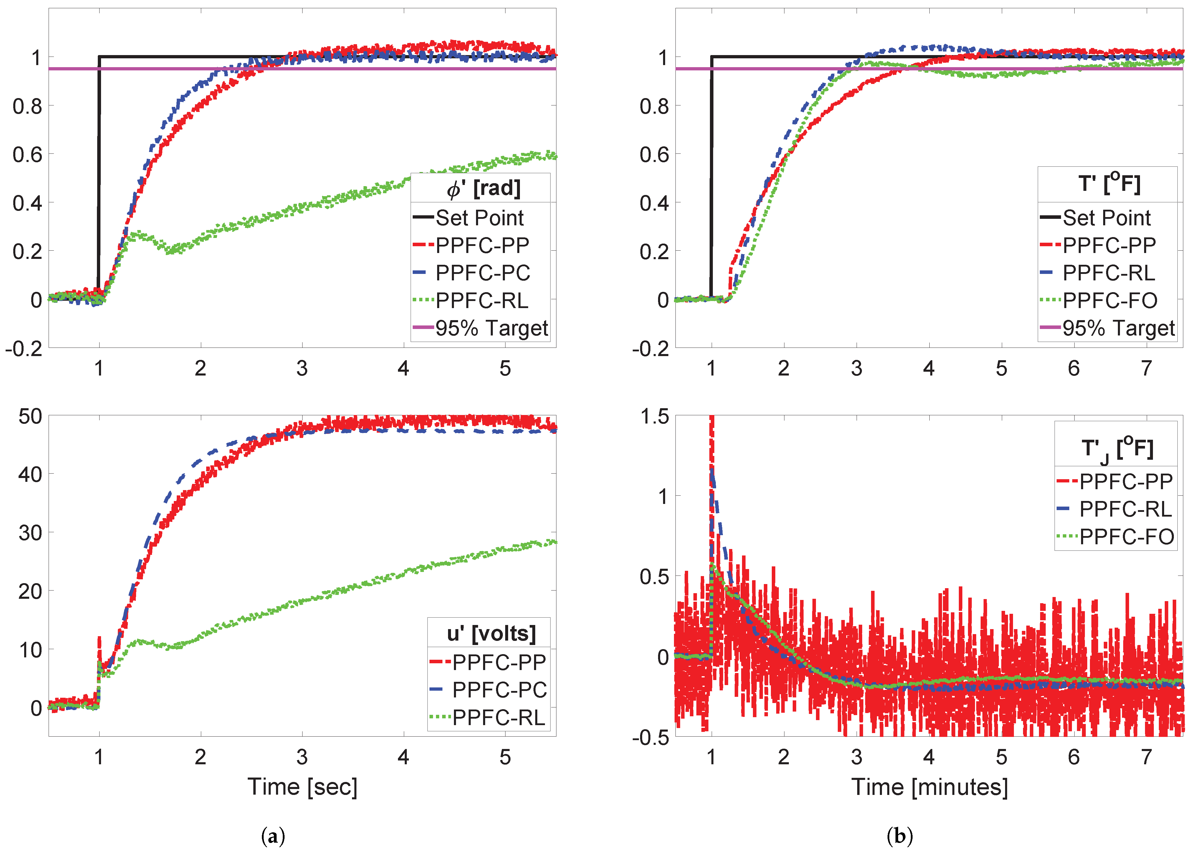
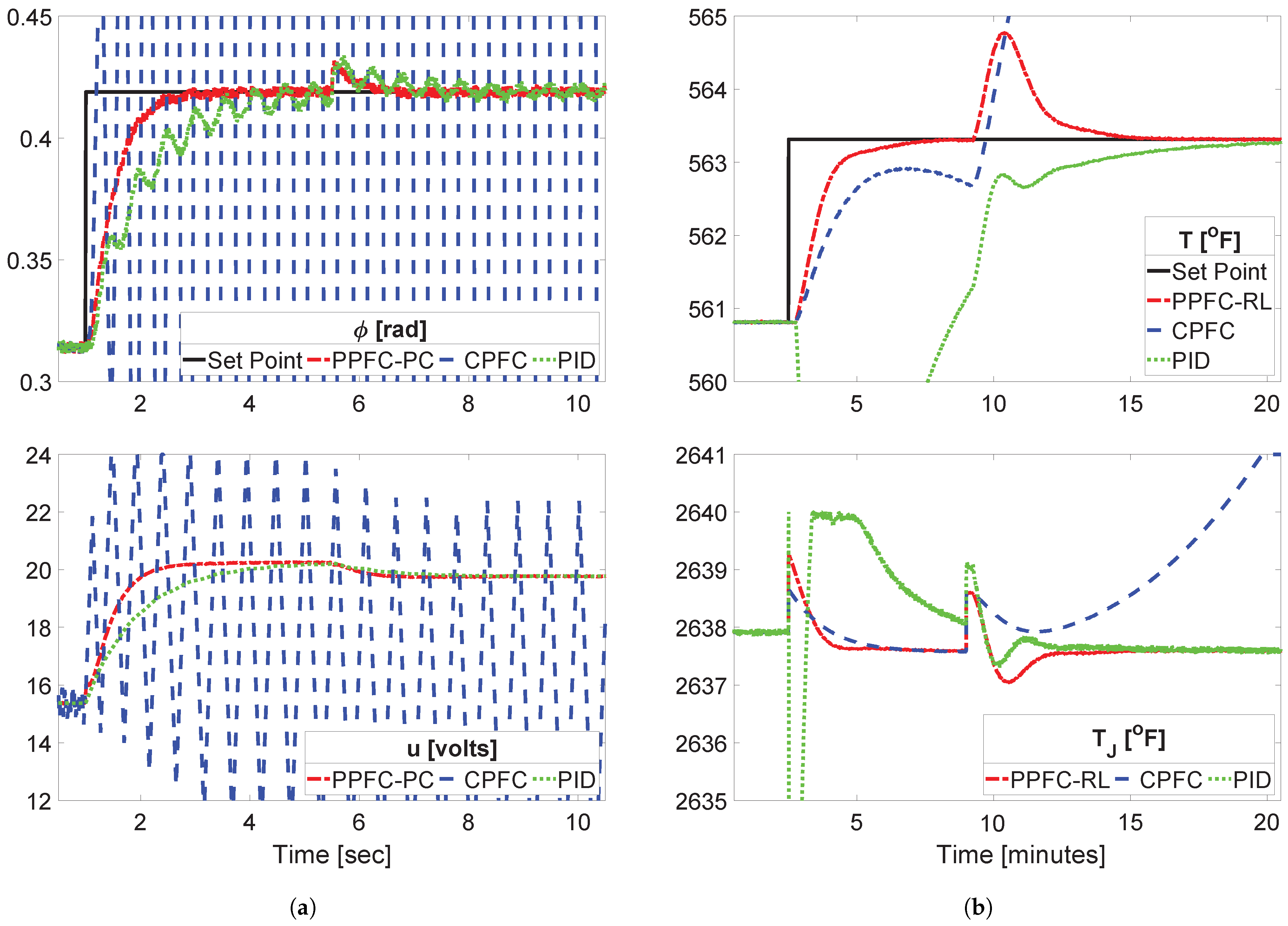
5.5. Analysis of Constrained Closed-Loop Performance

Based on the observations of the preceding sections, we selected PPFC-PC for the robotic arm example and PPFC-RL for the unstable CSTR system, and present a comparative analysis of the constrained closed-loop performance against the conventional PFC (CPFC) and PID controllers. For a fair comparison, the CPFC uses the parameters $\rho$ and $n_y$ chosen according to the corresponding $\theta$, albeit with difficult open-loop prediction dynamics implemented directly within the control law. Furthermore, the PID was synthesised using the robust PID tuning algorithm available in MATLAB [33]. The actual non-linear models (36) and (37) acted as the plants for a more realistic evaluation.

Figure 9a depicts the scenario for the poorly damped robotic arm process, where a set point change of 0.105 radians, i.e., 6°, from the initial steady-state was introduced. As evident, both the CPFC and PID controllers failed to compensate the open-loop underdamping, though the performance of CPFC was far worse under the constraints. On the other hand, the proposed PPFC not only successfully filtered out the unwanted oscillations, but did so by maintaining feasibility despite a significant change in both the set point and the disturbance.

For the unstable jacketed CSTR process, the closed-loop performance is displayed in Figure 9b. A step change of 2.5 °F drove the process away from the nominal operating point, causing large uncertainty, which alongside the imposed actuation limit proved too demanding for both the CPFC and the PID. In this case too, the proposed PPFC algorithm depicted superior performance, with highly commendable characteristics despite facing the challenges.

Thus, these examples validate the rationale behind using pre-stabilised predictions in predictive functional control law for a superior performance, as compared to the direct utilisation of the difficult open-loop dynamics, which clearly fails to fulfil the desired performance specification in an efficient and reliable manner.

6. Conclusions

This paper presents a dual-loop control architecture for challenging industrial processes that combine two seemingly different concepts, i.e., pre-stabilisation and relative tuning, in order to rectify the fundamental weaknesses of the conventional PFC algorithm. More specifically, the proposal transforms the difficult open-loop prediction dynamics via classical feedback compensation in an inner loop so as to obtain stable and well-damped prediction behaviour that is more easily manageable by the outer loop PFC. Moreover, the PFC employs a novel tuning technique that bases decision making relative to the steady-state benchmark performance of the pre-stabilised system, making the overall implementation much more transparent and intuitive than the original PFC, or indeed PID, in industrial settings.

The paper has also consolidated and summarised numerous simple and well-understood classical feedback compensation designs that work well within the proposed dual-loop control framework. Notably, the work highlights the superior efficacy of Pole Cancellation for poorly damped stable systems, which not only ensures reliable and consistent prediction dynamics but also provides excellent performance under the influence of disturbances, noise, and modelling uncertainties. For open-loop unstable processes, however, the recommendation is to implement reduced second- or first-order models, if possible, as compensating higher-order dynamics directly with Pole Placement often produces aggressive control action, which may in turn lead to constraint violation or instability in practice.

While the current simulation results are highly promising, in future, the authors plan to validate the proposal’s efficacy with hardware-based experiments on challenging industrial processes. Furthermore, we plan to investigate the functionality of inner-loop designs more closely using detailed frequency domain analysis so as to understand why pre-stabilisation based on Pole Cancellation performs so efficiently as compared to other techniques, especially in handling uncertainties and disturbances.

References

1. Richalet, J.; Rault, A.; Testud, J.; Papon, J. Model predictive heuristic control. Automatica 1978, 14, 413–428. [Google Scholar] [CrossRef]
2. Richalet, J.; O’Donovan, D. Predictive Functional Control: Principles and Industrial Applications; Springer Science & Business Media: Berlin/Heidelberg, Germany, 2009. [Google Scholar] [CrossRef]
3. Richalet, J.; O’Donovan, D. Elementary predictive functional control: A tutorial. In Proceedings of the 2011 International Symposium on Advanced Control of Industrial Processes (ADCONIP), Hangzhou, China, 23–26 May 2011; pp. 306–313. [Google Scholar]
4. Zhou, L.; Lin, J.; Sun, J.; Fu, H.; Wan, Q. Predictive Functional Control for Linear Motor Speed System Based on Repetitive Sliding Mode Observer. In Proceedings of the 2021 40th Chinese Control Conference (CCC), Shanghai, China, 26–28 July 2021; IEEE: Piscataway, NJ, USA, 2021; pp. 2633–2638. [Google Scholar] [CrossRef]
5. Luo, Q.; Bai, J.; Wu, F. Improved Constrained Predictive Functional Control Using Extended Non-Minimal State Space Formulation for the Cement Production Process. Processes 2022, 10, 969. [Google Scholar] [CrossRef]
6. Zainuddin, M.; Abdullah, M.; Ahmad, S.; Tofrowaih, K. Performance Comparison Between Predictive Functional Control and PID Algorithms for an Automobile Cruise Control System. Int. J. Automot. Mech. Eng. 2022, 19, 9460–9468. [Google Scholar] [CrossRef]
7. Li, H.; Song, B.; Chen, T.; Xie, Y.; Zhou, X. Adaptive fuzzy PI controller for permanent magnet synchronous motor drive based on predictive functional control. J. Frankl. Inst. 2021, 358, 7333–7364. [Google Scholar] [CrossRef]
8. Eduardo, F.; Camacho, C.B.A. Model Predictive Control; Springer: London, UK, 2007. [Google Scholar]
9. Mayne, D.Q. Model predictive control: Recent developments and future promise. Automatica 2014, 50, 2967–2986. [Google Scholar] [CrossRef]
10. Köhler, J.; Müller, M.A.; Allgöwer, F. Analysis and design of model predictive control frameworks for dynamic operation—An overview. Annu. Rev. Control 2024, 57, 100929. [Google Scholar] [CrossRef]
11. Nikolaou, M. Model Predictive Controllers: A Critical Synthesis of Theory and Industrial Needs. In Advances in Chemical Engineering; Elsevier: Amsterdam, The Netherlands, 2001; pp. 131–204. [Google Scholar] [CrossRef]
12. Rossiter, J.A. A First Course in Predictive Control; CRC Press: Boca Raton, FL, USA, 2018. [Google Scholar]
13. Rossiter, J.A.; Haber, R. The effect of coincidence horizon on predictive functional control. Processes 2015, 3, 25–45. [Google Scholar] [CrossRef]
14. Rossiter, J.A. Input shaping for PFC: How and why? J. Control Decis. 2016, 3, 105–118. [Google Scholar] [CrossRef]
15. Khadir, M.; Ringwood, J. Extension of first order Predictive Functional Controllers to handle higher order internal models. Int. J. Appl. Math. Comput. Sci. 2008, 18, 229–239. [Google Scholar] [CrossRef]
16. Zabet, K.; Rossiter, J.A.; Haber, R.; Abdullah, M. Pole-placement predictive functional control for under-damped systems with real numbers algebra. ISA Trans. 2017, 71, 403–414. [Google Scholar] [CrossRef] [PubMed]
17. Mayne, D.Q.; Rawlings, J.B.; Rao, C.V.; Scokaert, P.O. Constrained model predictive control: Stability and optimality. Automatica 2000, 36, 789–814. [Google Scholar] [CrossRef]
18. Rossiter, J.A.; Kouvaritakis, B.; Rice, M. A numerically robust state-space approach to stable-predictive control strategies. Automatica 1998, 34, 65–73. [Google Scholar] [CrossRef]
19. Aftab, M.S.; Rossiter, J.A. Predictive functional control for challenging dynamic processes using a simple prestabilization strategy. Adv. Control Appl. 2022, 4, e102. [Google Scholar] [CrossRef]
20. Aftab, M.S.; Rossiter, J.A. Predictive Functional Control with Explicit Pre-conditioning for Oscillatory Dynamic Systems. In Proceedings of the 2021 European Control Conference (ECC), Delft, The Netherlands, 29 June–2 July 2021; IEEE: Piscataway, NJ, USA, 2021. [Google Scholar] [CrossRef]
21. Zhang, Z.; Xie, L.; Lu, S.; Rossiter, J.A.; Su, H. A low-cost pole-placement MPC algorithm for controlling complex dynamic systems. J. Process Control 2022, 111, 106–116. [Google Scholar] [CrossRef]
22. Rossiter, J.A.; Abdullah, M.; Aftab, M.S. Improving the Feedforward Component for Recent Variants of Predictive Functional Control. Processes 2024, 12, 229. [Google Scholar] [CrossRef]
23. Aftab, M.S.; Rossiter, J.A.; Panoutsos, G. Predictive Functional Control for Difficult Dynamic Processes with a Simplified Tuning Mechanism. In Proceedings of the 2022 UKACC 13th International Conference on Control (CONTROL), Plymouth, UK, 20–22 April 2022; pp. 130–135. [Google Scholar] [CrossRef]
24. Aftab, M.S.; Rossiter, J.A.; Zhang, Z. Predictive Functional Control for Unstable First-Order Dynamic Systems. In CONTROLO 2020; Lecture Notes in Electrical Engineering; Springer International Publishing: Berlin/Heidelberg, Germany, 2020; pp. 12–22. [Google Scholar] [CrossRef]
25. Aftab, M.S.; Rossiter, J.A.; Panoutsos, G. Predictive Functional Control for Difficult Second-Order Dynamics with a Simple Pre-compensation Strategy. In Proceedings of the 2022 UKACC 13th International Conference on Control (CONTROL), Plymouth, UK, 20–22 April 2022; IEEE: Piscataway, NJ, USA, 2022. [Google Scholar] [CrossRef]
26. Ogata, K. Discrete-Time Control Systems, 2nd ed.; Prentice Hall Englewood: Cliffs, NJ, USA, 1995. [Google Scholar]
27. Nise, N.S. Control Systems Engineering, 6th ed.; John Wiley & Sons: Hoboken, NJ, USA, 2007. [Google Scholar]
28. Goodwin, G. Control System Design; Prentice Hall: Upper Saddle River, NJ, USA, 2001. [Google Scholar]
29. Hasirci, U. An engineering education tool for real-time nonlinear control: Stabilization of a single link robot. Int. J. Electr. Eng. Educ. 2015, 52, 320–339. [Google Scholar] [CrossRef]
30. Bequette, B. Behavior of a CSTR with a recirculating jacket heat transfer system. In Proceedings of the Proceedings of the 2002 American Control Conference (IEEE Cat. No.CH37301), Anchorage, AK, USA, 8–10 May 2002; IEEE: Piscataway, NJ, USA, 2002. [Google Scholar] [CrossRef]
31. Rao, A.S.; Chidambaram, M. Analytical design of modified Smith predictor in a two-degrees-of-freedom control scheme for second order unstable processes with time delay. ISA Trans. 2008, 47, 407–419. [Google Scholar] [CrossRef] [PubMed]
32. MathWorks. Model Reducer: Reduce Complexity of Linear Time-Invariant (LTI) Models. 2024. Available online: https://www.mathworks.com/help/control/ref/modelreducer-app.html (accessed on 3 February 2025).
33. MathWorks. PID Tuning Algorithm. 2024. Available online: https://www.mathworks.com/help/control/getstart/pid-tuning-algorithm.html (accessed on 3 February 2025).
Figure 1. Pre-stabilisation loop structure with compensation in (a) forward path, and (b) feedback path.
Processes 13 00862 g001
Figure 2. Dual-loop PFC control architecture.
Processes 13 00862 g002
Figure 3. Root locus design of a difficult second-order dynamic system with (a) complex pole pair, (b) one unstable pole.
Processes 13 00862 g003
Figure 4. Schematic representation of (a) DC motor-driven single-link robot, and (b) jacketed CSTR process.
Processes 13 00862 g004
Figure 5. Tuning efficacy of dual-loop PFC for single-link robotic arm process with Pole Placement, Pole Cancellation, and Root Locus compensation schemes using (a) θ = 1 (benchmark), and (b) θ = 5 .
Processes 13 00862 g005
Figure 6. Tuning efficacy of dual-loop PFC for jacketed CSTR process with Pole Placement, Root Locus, and First-Order compensation schemes using (a) θ = 1 (benchmark), and (b) θ = 3 .
Processes 13 00862 g006
Figure 7. Comparison of disturbance rejection between various compensation schemes for (a) single-link robotic arm with θ = 5 and a constant output disturbance of 0.1 rad, and (b) jacketed CSTR with θ = 3 and a constant input disturbance of 1 °F.
Processes 13 00862 g007
Figure 8. Comparison of tuning efficacy between various compensation schemes along with measurement noise and plant-model mismatches for (a) single-link robotic arm with θ = 5 and an unmodelled pole at z = 0.5 , and (b) jacketed CSTR with θ = 3 and a 10 % multiplicative uncertainty.
Processes 13 00862 g008
Figure 9. Closed-loop performance comparison with constraints and external perturbations for (a) single-link robotic arm pre-stabilised via Pole Cancellation using θ = 5 subject to | Δ u | 0.5 volts and 0 u 24 volts, and (b) jacketed CSTR pre-stabilised via Root Locus scheme with θ = 3 subject to T J 2640 °F.
Processes 13 00862 g009