Predicting Multi-Dense Jet Concentration Fields Using a Field Reconstruction Machine Learning Framework

Abstract

Jet phenomena have significant applications in environmental engineering, chemical process simulations, fluid dynamics, and pollutant dispersion. However, traditional physical models and numerical simulation methods face challenges such as high computational cost and limited accuracy when dealing with complex jet phenomena, such as systems with multiple inclined dense jets. To address this issue, this study proposes a field reconstruction machine learning algorithm to model the concentration field of multiple inclined dense jets. A comprehensive dataset was constructed through computational fluid dynamics (CFD) simulations, and a field reconstruction LightGBM model was trained and compared with field reconstruction approaches based on the XGBoost, GradientBoostingRegressor, and KNN algorithms to validate its superiority in this physical problem. Through testing, the R² value of LightGBM is close to 0.99, and the RMSE value is around 0.001. The results show that the LightGBM model can accurately predict the mixing and diffusion processes of the jets and exhibits higher prediction accuracy and stability compared to other machine learning methods used in this study, particularly in the complex flow environment of high-density jets. This study provides new ideas and tools for researching jet characteristics and offers theoretical support for engineering emission optimization.

1. Introduction

The behavior of jets has a significant impact on water quality monitoring, chemical process simulations, pollutant dispersion, and aquatic ecosystem management [1]. Inclined dense jets, as a common fluid dynamics phenomenon, require the accurate prediction of the concentration field variations for engineering design and environmental monitoring. However, high-density jets often experience large density differences, which make them prone to instabilities such as fluctuations and vortices [2], increasing the difficulty in predicting concentration fields.

Traditional mathematical methods, such as empirical formulas and analytical approaches, rely on certain assumptions or simplifications and cannot describe the turbulent mixing and momentum interference effects between multiple jets. Additionally, buoyancy plays an important role in high-density flows, and traditional methods struggle to predict this complex evolution accurately [3]. Numerical simulation methods require high computational precision and dense grids to capture details, especially in multi-jet systems, which demand vast computational resources. Moreover, in buoyancy-driven flows, the dynamic changes in jets require higher precision in computations, further increasing the model’s complexity and computational burden. In contrast, machine learning methods can automatically capture the complex interactions and dynamic changes between fluids by training on large datasets, without the need for manually defining specific physical models or assumptions. Data-driven modeling can reduce computational costs [4]. Therefore, machine learning methods hold promise for enhancing predictive capabilities in this field.

Early fundamental research has revealed the controlling effects of the tilt angle and density Froude number on geometric features such as jet trajectory and rise height through experiments [5,6]. Ferrari et al. [7] reported the phenomenon of re-entrainment in negative buoyant jets. Shao et al. [8], Jiang et al. [9], and Gungor et al. [10] conducted experimental studies on the mixing characteristics and turbulence properties of jets. Abessi et al. [11] studied the flow characteristics of single dense jets at different nozzle angles, while Pagliara et al. [12] revealed the multi-factor coupling mechanism of multi-jet erosion patterns. Papakonstantis et al. [13,14,15] systematically uncovered the radial expansion mechanism of jet impact on the bottom and the concentration distribution characteristics at different tilt angles. In terms of theoretical modeling, Lai et al. [16] established an empirical relationship between the mixing characteristics and dilution of circular density jets, while Kikkert et al. [17] proposed an analytical solution that could describe the jet trajectory but underestimated the internal expansion. These studies provide theoretical support and experimental evidence for jet characteristics, but their applicability in complex jet systems may be limited.

Computational fluid dynamics (CFD) methods can handle complex geometries, boundary conditions, and flow characteristics, offering greater flexibility and accuracy. Choi et al. [18] revealed the concentration field evolution of jet impact on the bottom in co-flow through experiments and 3D numerical models. Bombardelli et al. [19] and Ma et al. [20], respectively, combined experiments and numerical methods to study the jet erosion depth evolution theory and water jet-induced air flow characteristics. Zhang et al. [21,22] used Large-Eddy Simulation (LES) to analyze the turbulent mixing behavior of circular wall jets and 45° and 60° inclined dense jets, while Liu et al. [23] captured the free-falling jet morphology precisely using finite element and level set methods. Yan et al. [24] conducted a series of numerical simulations to study jet characteristics in various scenarios. Additionally, Nikiforakis et al. [25] improved the prediction accuracy of negative buoyant jets by modifying the CorJet model, Lou et al. [26] established a merged plume model to reveal the effect of buoyant flux on turbulent entrainment, and Li et al. [27] clarified the flow field and scour coupling process of wall jet erosion through numerical simulation. These studies demonstrate that CFD simulations can be conducted in complex flow domains, providing more detailed flow field information compared to traditional methods, though they require significant computational resources and time.

In recent years, machine learning has gradually been applied in the field of fluid mechanics [4]. Yan et al. [28] researched the application of multi-gene genetic programming (MGGP) technology in jet characteristic modeling and prediction, showing that machine learning can make rapid predictions and significantly improve computational efficiency compared to numerical simulations. However, the performance of different algorithms varies, and when predicting the concentration field of multiple inclined dense jets, large-scale data processing is required. A challenge is how to reduce training time and memory consumption while ensuring prediction accuracy. LightGBM, a gradient-boosting tree-based machine learning algorithm, is particularly suitable for handling large-scale datasets and has been applied across various fields [29,30,31,32]. However, current studies have not applied machine learning methods to simulate the concentration field of multiple inclined dense jets, nor have they used LightGBM models to predict jet phenomena.

To validate the potential of machine learning methods in complex flow problems, this study used field reconstruction machine learning to simulate the concentration fields of multiple inclined dense jets. Simulating the concentration fields of multiple inclined dense jets is a crucial and challenging problem. On one hand, this problem is essential for practical applications, such as in environmental protection, industrial production, and climate research, where understanding the concentration distribution of dense jets can help optimize resource utilization and control pollution. On the other hand, this problem also holds significant importance for machine learning research, as it presents a complex, multivariable, highly nonlinear, and time-varying system, which provides an excellent test case for evaluating the generalization capabilities of machine learning methods.

Therefore, this study proposes a field reconstruction machine learning framework that combines physics-driven feature engineering, enabling traditional machine learning models to efficiently perform field reconstruction. Specifically, it predicts the concentration field of multiple high-density inclined jets based on the field reconstruction LightGBM algorithm. First, concentration field data for 25 different jet densities were generated through OpenFOAM simulations, and 20 cases were randomly selected as the comprehensive dataset to train the model, with the remaining 5 cases used as unseen data to assess the model’s prediction performance. Then, the LightGBM algorithm was compared with other machine learning algorithms to verify its advantages in this physical problem. To the best of the authors’ knowledge, this is the first application of the LightGBM algorithm to predict multi-dense jet concentration fields inclined dense jets. This method significantly improves computational efficiency while maintaining prediction accuracy. This study provides a new method for predicting inclined dense jets and offers new research ideas for the prediction of other complex fluid problems.

2. Materials and Methods

2.1. Overall Research Approach

This study proposes a field reconstruction machine learning framework based on existing machine learning algorithms. Through feature selection engineering, we developed a field reconstruction LightGBM algorithm and applied it to the simulation and prediction of multiple inclined dense jets concentration fields. The research approach is shown in Figure 1 and consists of three main stages: CFD simulation and model validation, data preparation and preprocessing, and machine learning modeling. First, CFD simulations were conducted to model the concentration field of inclined dense jets under different conditions, generating concentration field data for various scenarios. The data were then normalized, and feature extraction was performed to build a comprehensive dataset, laying the foundation for subsequent machine learning model training. Then, an efficient concentration field reconstruction machine learning model was constructed based on the LightGBM algorithm through feature selection. The model’s prediction accuracy was enhanced through model training and hyperparameter optimization. The model’s performance was evaluated using multiple metrics, and the LightGBM algorithm was compared with other machine learning models to verify its superiority in predicting the concentration field of multiple inclined dense jets.

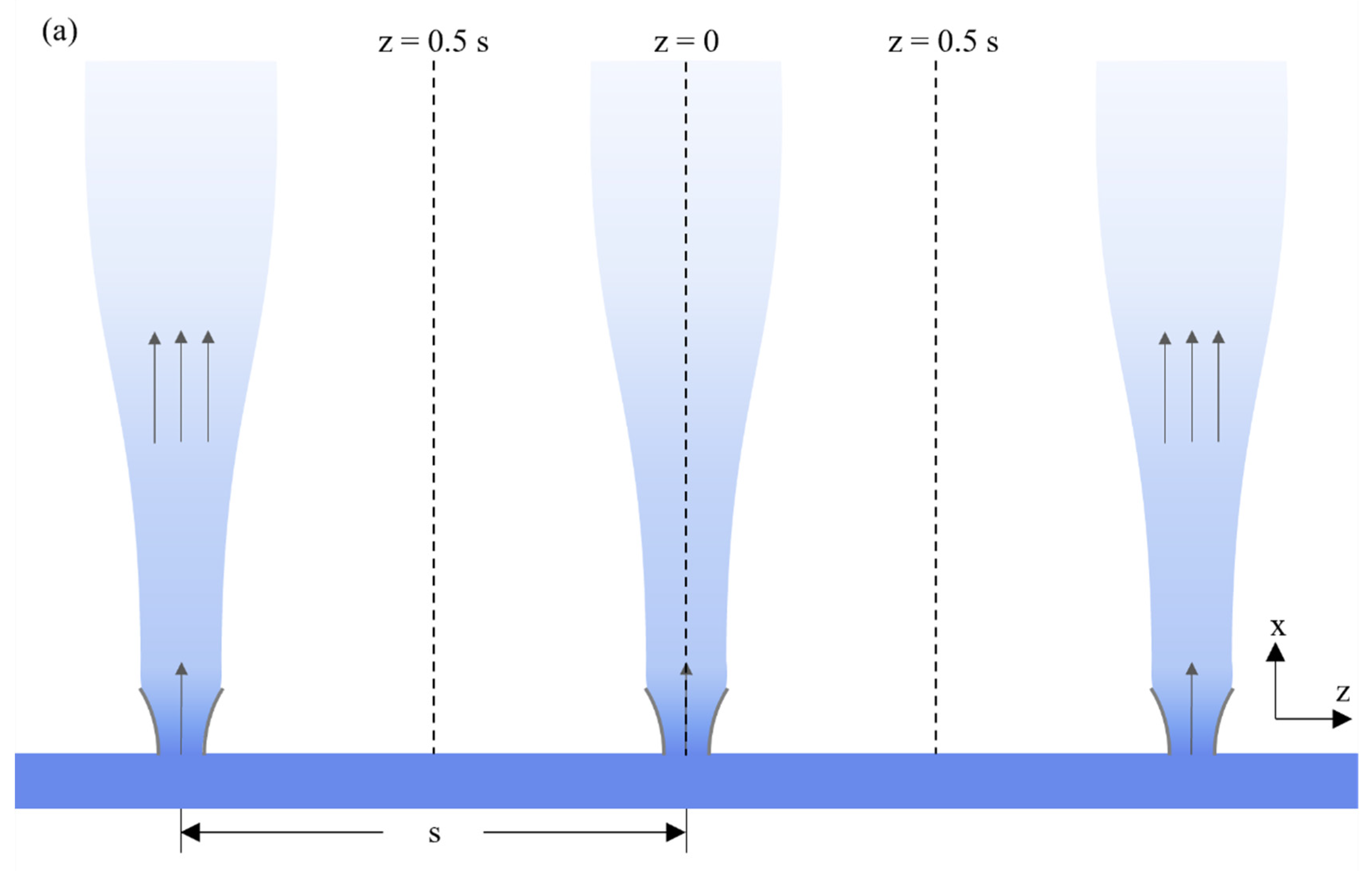
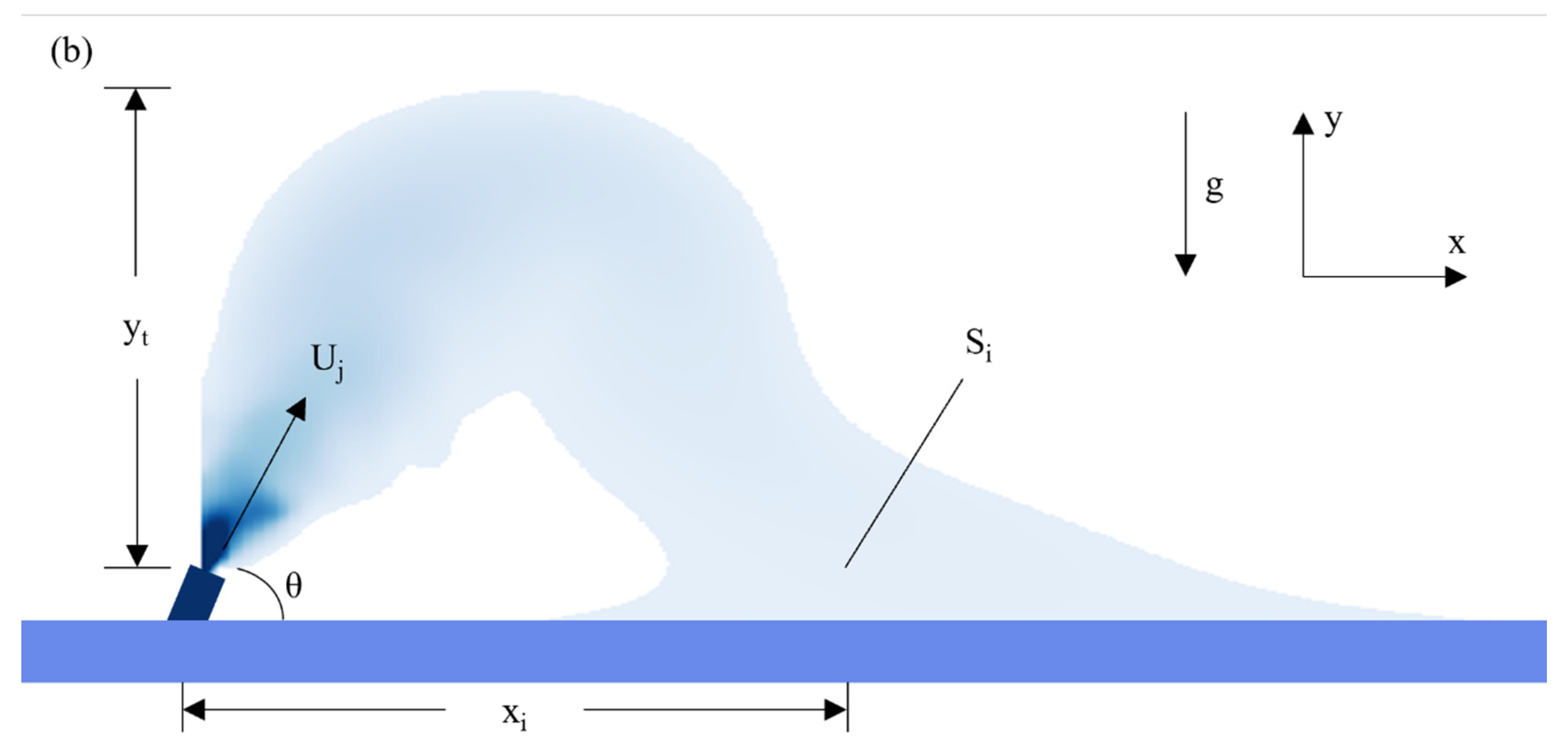
2.2. Physical Phenomenon

Schematics of multiple inclined dense jets are shown in Figure 2, where (a) is the plan view and (b) is the elevation view. These jets are ejected from multiple nozzles spaced at a distance s with an angle θ and initial velocity U_j into the surrounding water. After reaching the highest point, they fall back to the horizontal bed. The height at the highest point is referred to as the terminal rise height (y_t), the distance between the diffuser nozzle and the reattachment point is called the impact distance (x_i), and the dilution at the reattachment point is referred to as the impact dilution (S_i).

2.3. Physical Representation

In this study, CFD simulations were conducted within the OpenFOAM (version 11) framework. It was assumed that the multiple fluids are incompressible and Newtonian. In this study, multiple fluids refer to the receiving water body and the jet. Their physical properties were identical except for their density. The viscosity and density of the fluids were assumed to be constant, with the viscosity and density of the mixed fluid depending on the proportion of each fluid. These assumptions are reasonable for the current case. The three-dimensional Navier–Stokes equations for multiphase flow can be written as [33,34]

$$\nabla \cdot \mathrm{U}=0$$

(1)

$${\displaystyle \frac{\partial \rho \mathrm{U}}{\partial t}}+\nabla \cdot \left(\rho \mathrm{UU}\right)=-\nabla \cdot \left(p_{rgh}\right)-gh\nabla \rho +\nabla \cdot \left(\rho \mathrm{T}\right)$$

(2)

where U is velocity, ρ is density, and t denotes time. The term p_rgh represents static pressure minus hydraulic pressure, and h is the height of the fluid column.

The density ρ is calculated as the weighted average of the densities of the two fluids. Specifically, the density is the volume fraction α₁ of fluid 1 multiplied by its density ρ₁, plus the volume fraction α₂ of fluid 2 multiplied by its density ρ₂. The stress tensor T is the sum of three parts: the first part is the effective viscosity μ_eff multiplied by the divergence of the velocity gradient (∇⋅U) and the unit matrix I, which is then multiplied by the coefficient −2/3; the second part is the product of the effective viscosity and the velocity gradient ∇U; and the third part is the product of the effective viscosity and the transpose matrix of the velocity gradient (∇U)^T. The effective viscosity μ_eff is the weighted average of the effective viscosities of the two fluids. For a single fluid, the effective viscosity (μ_eff)_i is the dynamic viscosity μ minus the turbulent viscosity μ_t.

The volume fraction of the fluid is represented by the variable α, and the diffusion equation can be written as [24]

$${\displaystyle \frac{\partial \alpha }{\partial t}}+\nabla \cdot \left(\mathrm{U}\alpha \right)=\nabla \cdot \left(\left(D_{ab}+{\displaystyle \frac{{\nu }_t}{S_C}}\right)\nabla \alpha \right)$$

(3)

where D_ab is the molecular diffusivity, ν_t is the turbulent eddy viscosity, and S_C is the turbulent Schmidt number.

2.4. Numerical Experiments

The CFD simulation governing equations were solved using the “twoLiquidMixingFoam” solver in OpenFOAM, which has a high accuracy for predicting the mixing behavior of wastewater jets [35,36]. The computational domain was discretized using a fine hexahedral mesh with a port spacing of 0.114 m, and the total number of computational cells was 194,400. The default time step was set to 0.005 s, and the “adjustTimeStep” feature in OpenFOAM automatically was used to adjust the time step based on the maximum Courant number. To ensure smaller time steps, the maximum Courant number was set to 0.5 [24]. This study used the Latin hypercube design to investigate 25 different operating conditions, as shown in

Table 1. Operating condition design.

Cases	ρjet	Fr	s/(d·Fr)	Cases	ρjet	Fr	s/(d·Fr)
C00	1029	81.1	0.73	C13	1336	24.9	2.37
C01	1021	93.8	0.63	C14	1362	24.0	2.46
C02	1047	64.9	0.91	C15	1388	23.2	2.54
C03	1076	51.7	1.14	C16	1414	22.5	2.63
C04	1103	44.6	1.32	C17	1440	21.8	2.71
C05	1129	40.0	1.48	C18	1466	21.2	2.79
C06	1154	36.6	1.61	C19	1492	20.6	2.86
C07	1180	33.9	1.74	C20	1518	20.1	2.94
C08	1207	31.7	1.86	C21	1544	19.6	3.01
C09	1233	29.9	1.98	C22	1570	19.2	3.08
C10	1259	28.4	2.08	C23	1596	18.8	3.15
C11	1276	27.5	2.15	C24	1622	18.4	3.22
C12	1310	25.9	2.28	C25	1649	18.0	3.29

Note: ρ_jet = jet density; F_r = density Froude number; d = diameter; s = port spacing.

, with C00 being the baseline case, and the U_x for each case was 1 m/s, while U_y was 1.7321 m/s.

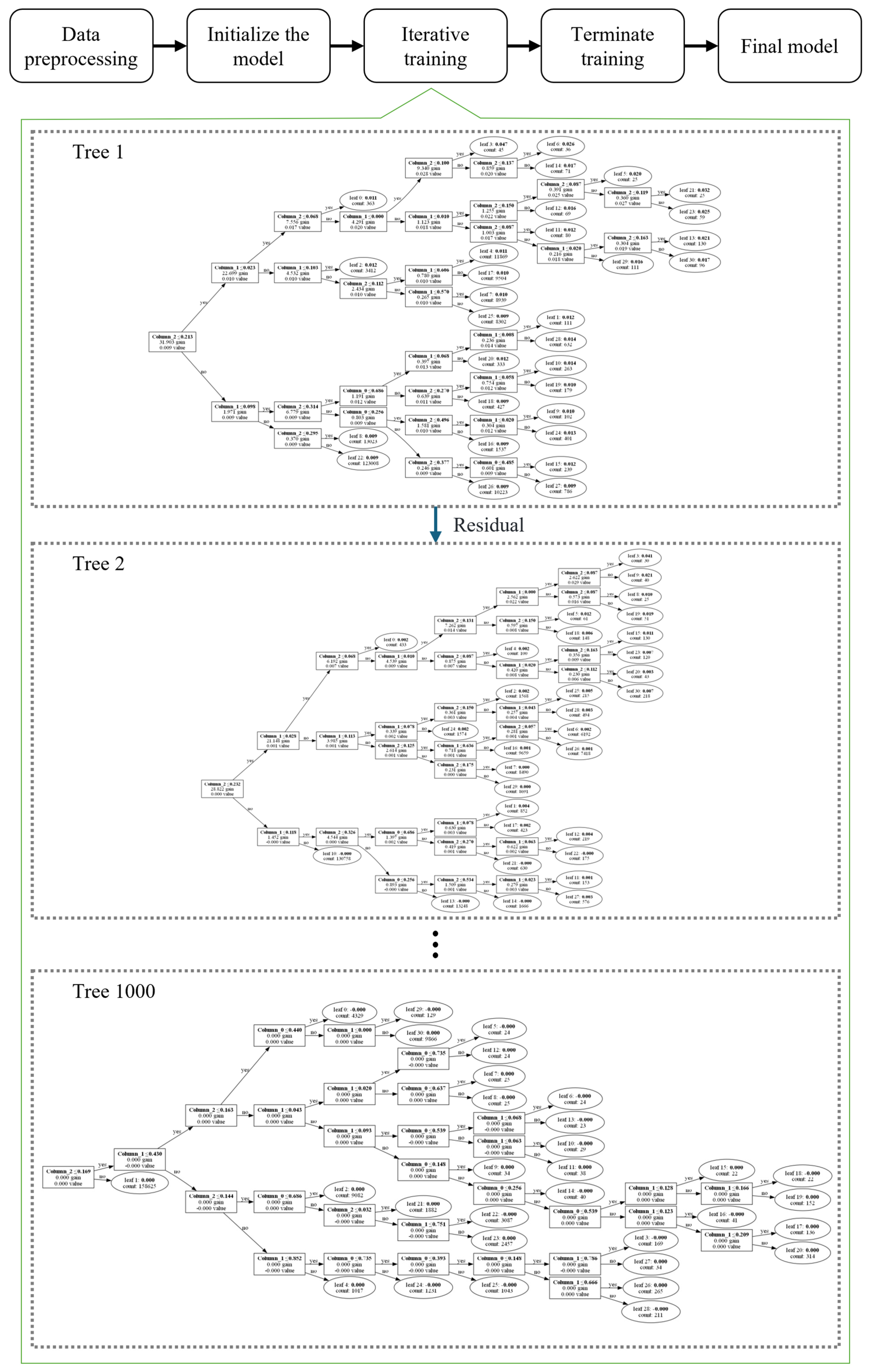
2.5. Field Reconstruction LightGBM Algorithm

Light Gradient-Boosting Machine (LightGBM) is an efficient machine learning algorithm based on gradient-boosting trees (GBTs). It combines multiple decision tree models to make predictions, reducing bias and variance, thereby improving the model’s generalization ability. In this study, the LightGBM algorithm was used to simulate the concentration field of multiple inclined dense jets. Through feature selection, LightGBM can achieve concentration field reconstruction. Specifically, the s/(dF) value, x-coordinate, and y-coordinate were selected as features and normalized. The algorithm flowchart is shown in Figure 3.

First, the data were preprocessed, and the model was initialized with the number of decision trees set to 1000 and the learning rate set to 0.05 to ensure the model’s learning ability and stability. During the iterative training process, each iteration calculates the negative gradient of the current model as the new target value and seeks the optimal split point based on the binned histogram to build the decision tree. The tree growth follows the leaf-wise strategy, selecting the optimal split based on gradient gain. Parameters num_leaves and max_depth were set to 31 and −1 to avoid overfitting. The predicted results from the newly generated trees were scaled by the learning rate (η) and accumulated in the model, progressively optimizing it until the set number of trees was reached and training was stopped. Finally, the model, composed of multiple decision trees, is output. This method has good handling capability for large-scale data and can efficiently predict the concentration field of multiple inclined dense jets.

2.6. Reference Methods

2.6.1. GradientBoostingRegressor

GradientBoostingRegressor is a classic implementation of the gradient-boosting decision tree (GBDT), which enhances model performance by constructing multiple decision trees. Each newly generated tree corrects the residuals from the previous tree. Unlike LightGBM, GBDT uses a “level-wise growth” strategy to generate trees, starting from the root node and expanding the tree depth layer by layer. The number of nodes at each layer is the same until the maximum depth or other stopping criteria are reached. In this study, a GBDT model was built to simulate the concentration fields of multiple inclined dense jets. The number of decision trees was set to 100 to control model complexity, the learning rate was set to 0.1 to adjust the contribution of each tree to the overall model, and the maximum depth of the trees was set to 3 to limit the complexity of each tree and prevent overfitting. The model was trained using a normalized training dataset, optimizing performance by progressively fitting the residuals of the training data.

2.6.2. XGBoost

eXtreme Gradient Boosting (XGBoost) is an enhanced version of GBDT. In addition to implementing gradient-boosting trees, it introduces L1 and L2 regularization to control model complexity and reduce the risk of overfitting. During the training process, two strategies—feature parallelism and data parallelism—are used to accelerate training and provide more efficient parallelization support. In this study, an XGBoost regression model was built with the objective function set to reg:squarederror to minimize squared error. The random seed was set to random_state = 42 to ensure the results of model training are reproducible. During model training, the normalized training data were used as input, where the target variable was flattened into a one-dimensional array to meet XGBoost’s input format requirements. The model was trained using the model.fit method, optimizing the decision tree structure through gradient boosting to learn the complex feature relationships in the data.

2.6.3. K-Nearest Neighbors

K-Nearest Neighbors (KNN) is an instance-based, non-parametric algorithm. Its core idea is to calculate the distance between a sample point and its neighboring data points and use the attributes of the k-nearest sample points to predict the value of the target variable. In this study, a KNN regression model was built to predict the concentration field of multiple inclined dense jets, with k = 5, meaning that the 5 nearest neighbors to the input sample are chosen for prediction, balancing the model’s fitting ability and robustness to noise. During the training phase, the model stores all sample data and their corresponding target values from the training set. During the prediction phase, the model finds the 5 nearest neighbors based on the distance between the test sample and the training samples, calculates the average of the target values of these neighbors, and returns this value as the prediction result.

3. Results

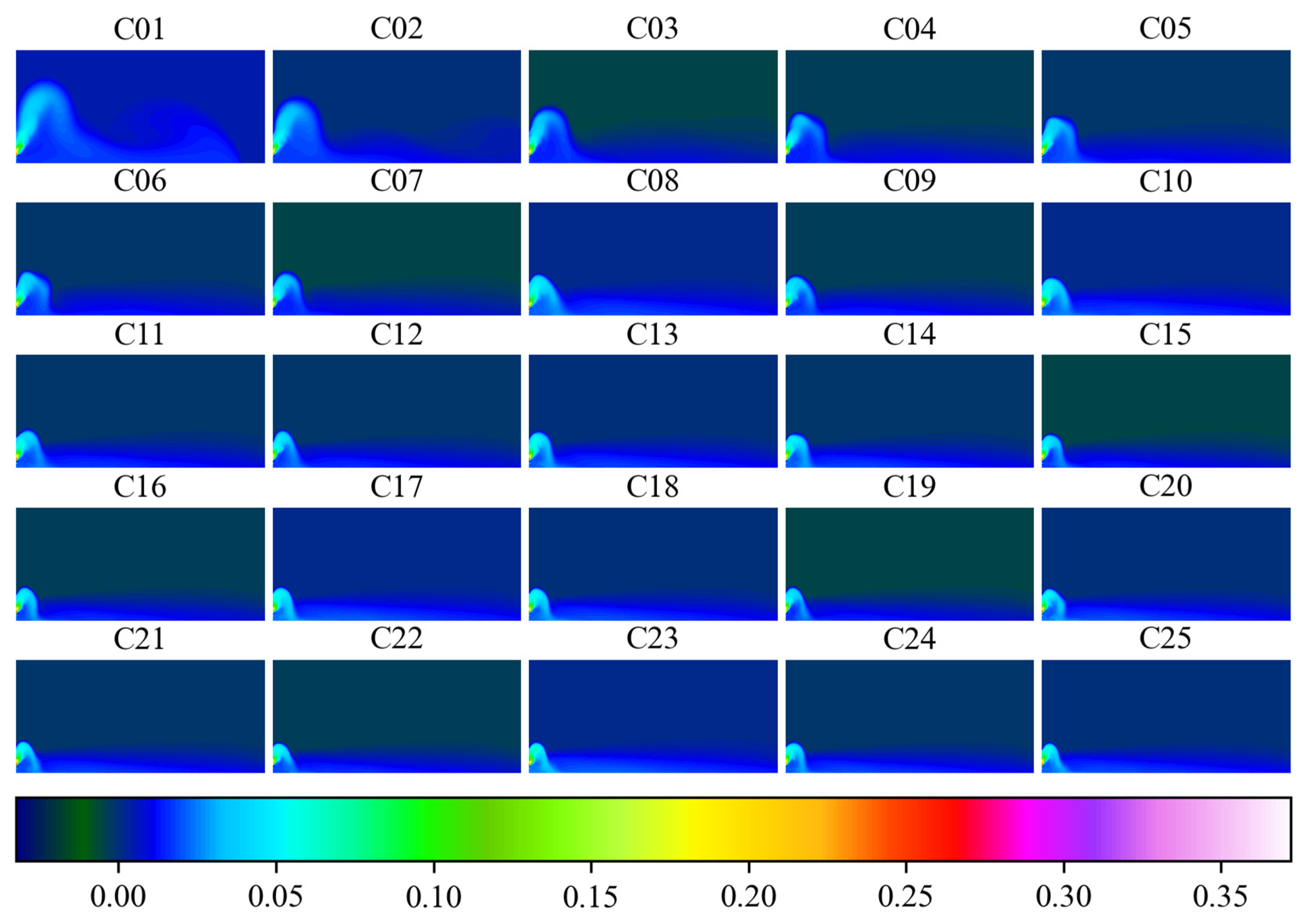
3.1. Numerical Results

Yan et al. [24] validated a numerical model, and the simulation results were consistent with experimental observations. They also calculated the relevant error metrics (MBE = −0.22, MAE = 0.22, MAPE = 11.81%, RMSE = 0.26, NRMSE = 0.14%, R² = 0.91), indicating that the numerical model has high reliability and can effectively capture the overall flow and mixing characteristics of multiple inclined dense jets. The validated CFD model was then utilized in this study to perform 25 additional scenarios.

Figure 4 shows the spatial distribution characteristics of the jet under different operating conditions. It can be seen that the C01–C05 jets have relatively low jet density, with the jets spreading more along the inclined direction and diffusing rapidly. The concentration gradient in the far-field region of the jet is relatively mild, indicating good mixing. For the C06–C15 jets, the jet density increases, and the depth of the jet’s descent also increases. The Froude number (Fr) lies between momentum-dominated and buoyancy-dominated regimes, showing both significant horizontal diffusion and a strong downward trend. For the C16–C25 jets, the jet density is higher, and the jets rapidly descend and spread along the bottom, exhibiting strong buoyancy effects. Overall, high-density jets show a stronger diving characteristic in the initial stage, while low-density jets have more noticeable diffusion. These results are consistent with existing theory and provide a reliable, comprehensive dataset for subsequent machine learning simulations.

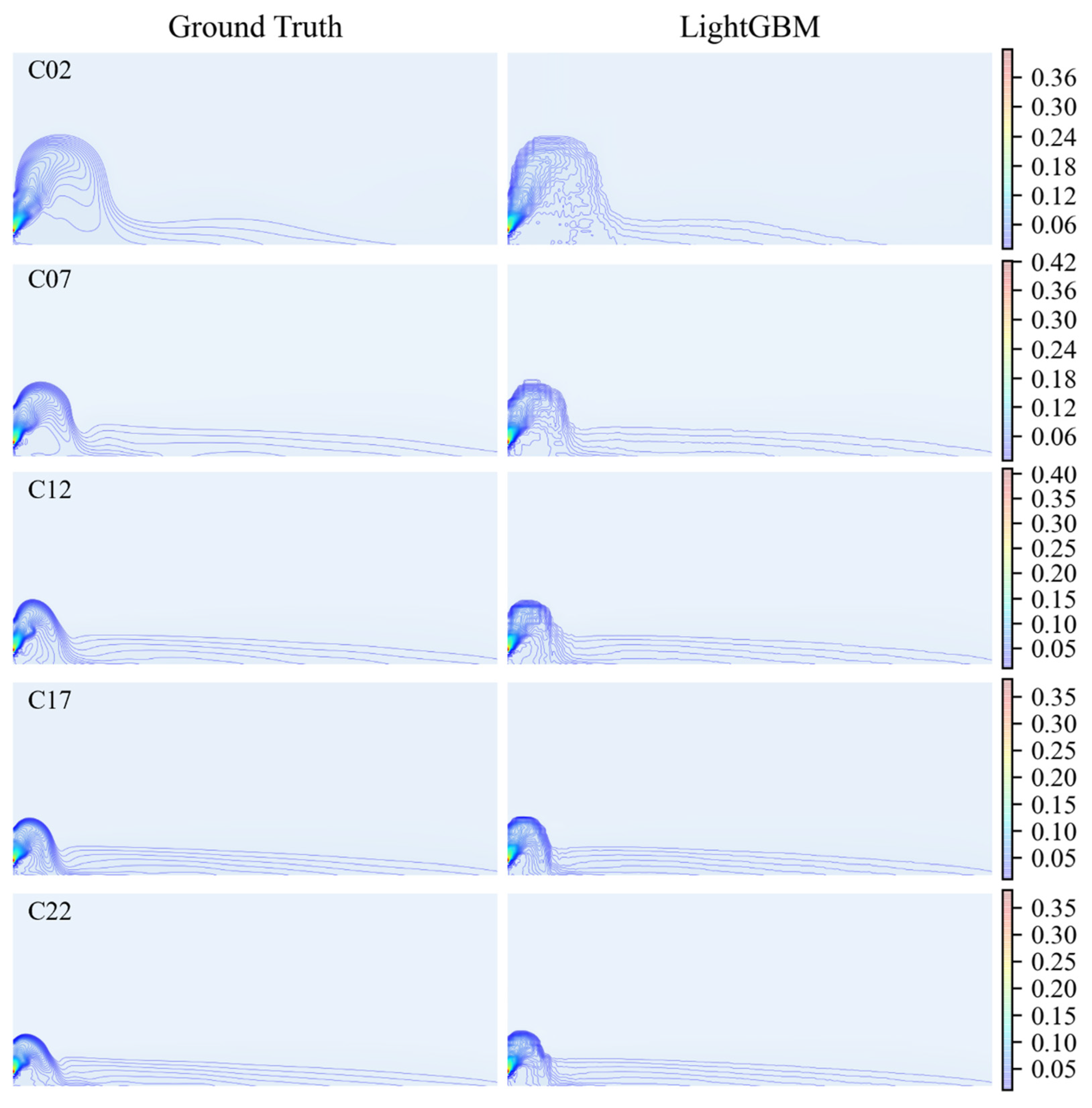
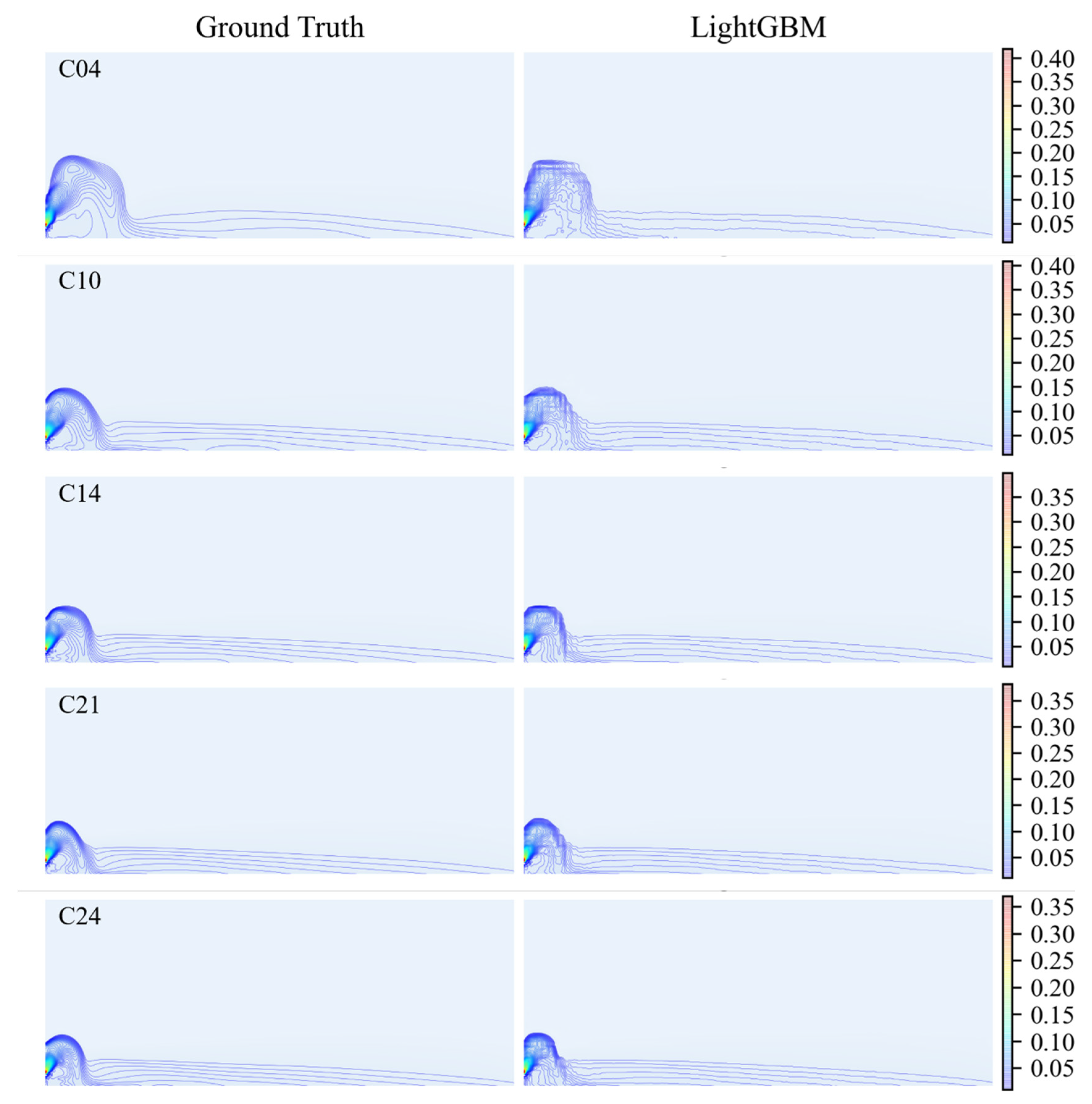
3.2. Performance of the LightGBM Method

To evaluate the performance of the LightGBM model, 20 out of 25 cases were randomly selected to construct a comprehensive dataset (with a total of 324,000 data points). The dataset was divided into training, validation, and test sets in a 6:2:2 ratio, with the remaining five cases used as unseen data to test the model’s prediction performance (with a total of 81,000 data points). Five cases were randomly selected from the comprehensive dataset, and the concentration field spatial distribution predicted by the LightGBM model was compared with the ground truth, as shown in Figure 5. At the jet source, the contour lines are spaced closely together, with large concentration changes and steep concentration gradients. As the jet expands into the far field, the spacing between the contour lines gradually increases, and the concentration changes slow down, indicating that the attenuation effect of the concentration begins to show, and the mixing of the jet with the surrounding fluid becomes more complete. The C02 concentration field exhibits typical jet diffusion characteristics. For C07 and C12, the jet density increases, the diffusion slows down, and the concentration distribution shows an obvious downward trend. For C17 and C22, the jet density is higher, showing a sinking effect, and the diffusion of the jet mainly occurs at the bottom, gradually expanding along the bottom in areas with higher concentration. The concentration attenuation in the far field is relatively slow. The LightGBM model’s predicted results are similar to the ground truth, effectively capturing the diffusion trend and concentration distribution of the ground truth concentration field.

To assess the predictive performance of the LightGBM model on unseen data, the prediction results for the remaining five cases were compared with the ground truth, as shown in Figure 6. From the figure, it can be seen that the LightGBM model successfully captured the concentration attenuation trend, effectively simulating the concentration diffusion trend, and accurately captured the concentration distribution of the jet in the near-source region. This indicates that the LightGBM model can effectively predict the concentration field of inclined dense jets.

To further assess the predictive performance of the LightGBM model, contour scatter plots were created, as shown in Figure 7. The LightGBM model performs excellently on both the integrated and unseen datasets. In the integrated dataset, the model’s R² value is generally close to 0.99, and the RMSE value is very low, indicating that the model fits the training data very well, with predictions almost identical to the real data. For the unseen data, although the R² value slightly decreases, it still remains high at around 0.98, and the RMSE value remains low, demonstrating the model’s strong generalization ability and its capability to accurately predict the concentration field variations in the unseen data. In both the training and unseen datasets, the data points are close to the 1:1 line, showing the model’s accuracy and stability in predictions. Overall, the LightGBM model not only performs excellently on the comprehensive dataset but also demonstrates strong predictive power and good generalization ability on the unseen dataset.

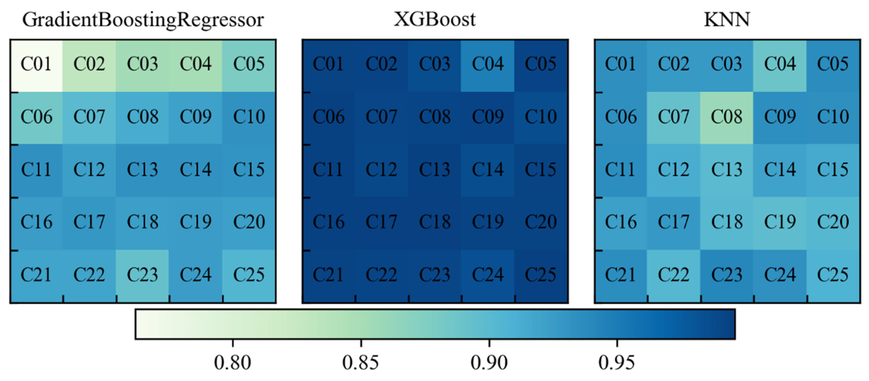
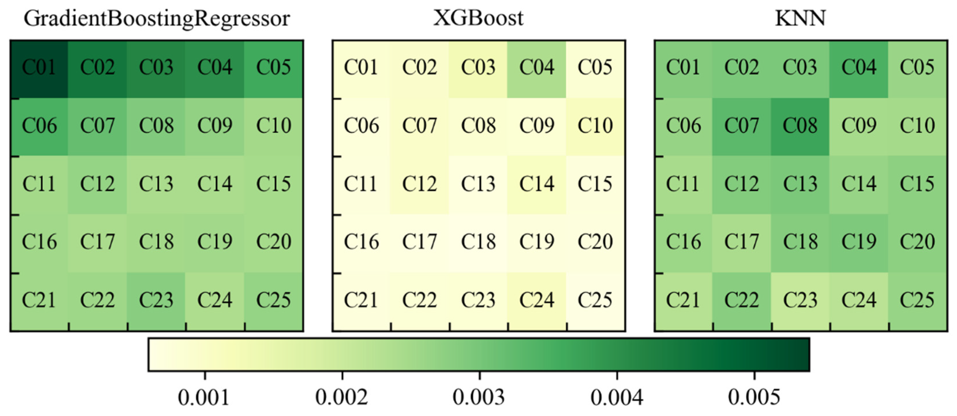
3.3. Performance of the Reference Methods

To analyze the performance of the GradientBoostingRegressor, XGBoost, and KNN models on different datasets, the R² values and RMSE values for each algorithm across different datasets were calculated, with the results shown in Figure 8 and Figure 9. All three algorithms performed well overall, with the XGBoost model performing the best, achieving an R² value close to 1 and the smallest RMSE error, indicating good fit and low error. However, in some individual cases, such as C04, the R² value decreased and the RMSE value increased. The GradientBoostingRegressor model showed poor prediction performance in low-density jets (C01–C05), but as the jet density increased, the R² value improved and the RMSE value decreased. On the other hand, the KNN model performed relatively weakly, with poor fitness and large errors in some cases (e.g., C08, C07), indicating its weaker adaptability in certain situations.

4. Discussion

This study is the first to apply machine learning algorithms to the reconstruction of concentration fields for multiple inclined dense jets. Specifically, the LightGBM algorithm was used to predict the concentration field of multiple inclined dense jets. As a nonlinear model, LightGBM can accurately simulate the distribution characteristics of the concentration field by learning the nonlinear relationship between the jet features and the concentration distribution. In the simulation of the concentration field of multiple inclined dense jets, the large volume of data was effectively processed by the model’s efficient gradient-boosting decision tree method, which significantly improves computational speed and efficiency when handling large-scale data. This provides a new and efficient solution for predicting concentration distributions in complex flow scenarios.

Traditional jet analysis methods, such as experimental studies, theoretical analysis, and numerical simulations, have certain limitations when predicting the concentration fields of multiple inclined dense jets. Experimental simulation methods allow for intuitive observation of jet behavior but typically require expensive equipment and substantial resources, making them costly. Moreover, experiments are often conducted on scaled-down models, which may lead to scale effects, making it difficult to accurately simulate jet behavior in real-world applications. Theoretical analysis is typically based on simplified assumptions, making it challenging to capture the complex interactions and nonlinear effects between fluids. Additionally, in multi-jet systems, obtaining a closed-form analytical solution is difficult, meaning that theoretical analysis may rely on approximate solutions or numerical methods, which may not fully describe the actual situation. High-precision numerical simulations require significant computational resources and time, especially when simulating multiple jets, which leads to high computational costs and time consumption. Compared to traditional methods, machine learning methods excel at capturing and modeling complex nonlinear relationships and can effectively simulate the dynamic behavior of multiple inclined jets. After training, machine learning models are usually faster in prediction than traditional numerical simulations, significantly reducing computational resource consumption. Therefore, compared to traditional methods, machine learning methods can reduce computational time while ensuring prediction accuracy, offering better adaptability and generalization ability.

To further analyze the predictive performance of the LightGBM algorithm compared to other machine learning algorithms for this physical problem, two-dimensional kernel density estimation (KDE) plots of the R² and RMSE for each algorithm are presented, as shown in Figure 10. The two-dimensional kernel density plot shows the joint distribution of the RMSE and R², rather than the direct numerical values. Therefore, when the R² value approaches 1, the smoothing effect caused by the KDE interpolation can make the kernel density plot show R² values exceeding 1, which is not the actual R² value. From the figure, it can be observed that both LightGBM and XGBoost perform excellently in predicting the concentration fields of multiple inclined dense jets. LightGBM, in particular, shows that most cases are concentrated in the high-R² (close to 1) and low-RMSE (close to 0.001) regions, indicating a very high degree of fit and accuracy in concentration field prediction. XGBoost also demonstrates high fitting performance, with R² close to 1, but with a slightly higher RMSE than LightGBM. In contrast, the GradientBoostingRegressor exhibits relatively poor fitting performance, with the data points being more scattered, and R² values concentrated between 0.85 and 0.95, which are relatively low, and a higher RMSE, indicating lower prediction accuracy. KNN performs relatively weakly, with R² values generally lower than 0.95 and higher RMSE, indicating that this model has poor accuracy in predicting concentration fields and struggles to capture the complex characteristics of high-density jets. Overall, LightGBM performs significantly better than other algorithms in this task, providing more accurate prediction results for the concentration field reconstruction of inclined dense jets.

In addition to being compared with other field reconstruction models based on traditional machine learning algorithms, LightGBM was further compared with deep learning algorithms (CNN). A CNN consisting of two convolutional layers (Conv1D), a flattening layer (Flatten), a fully connected layer (Dense), and a dropout layer was constructed. The model was trained using the Adam optimizer and the mean squared error (MSE) loss function. LightGBM and the CNN were trained on a computer equipped with a 13th-generation Intel(R) Core(TM) i5 processor and 16 GB of memory. In terms of computational efficiency and resource consumption, the LightGBM model only required a few minutes, while the CNN took more than 30 min. The results show that in the complex multi-jet concentration field reconstruction problem, the computational efficiency of LightGBM is significantly superior to that of the CNN, with the training time reduced several times. It can significantly outperform the more computationally expensive deep learning method (CNN) without sacrificing accuracy. This result further highlights the efficiency and application potential of LightGBM in concentration field reconstruction.

The core innovation of this study lies in the proposed efficient field reconstruction method, which can predict the concentration field of high-density jet flows with high efficiency using traditional machine learning methods (such as LightGBM) without relying on complex deep learning models. Traditional methods, such as CFD numerical simulations, are computationally expensive, while deep learning models often depend heavily on large datasets and involve high training costs. This study demonstrates that through utilizing relatively lightweight traditional machine learning methods like LightGBM, high-precision jet flow field predictions can be achieved, providing a low-cost and efficient alternative for related fields. While this study focused on the prediction of concentration fields in multiple inclined dense jets, the proposed field reconstruction approach using traditional machine learning techniques has broader applicability beyond this specific problem. The methodology of feature selection and efficient regression modeling can be extended to other fluid dynamics applications, such as pollutant dispersion, thermal plume modeling, and turbulence closure modeling. However, the diversity of the dataset in this study is relatively limited. In the future, the model’s generalization ability can be further improved by expanding the dataset and including data from different operating conditions and environmental factors. Additionally, new methods based on deep learning algorithms, such as neural networks, could be considered, as these methods may help study the complex scenarios involving multi-scale and multi-physical process coupling in aquatic environments.

5. Conclusions

This study applies machine learning methods to the reconstruction of multiple inclined dense jet concentration fields, builds a field reconstruction LightGBM machine learning model, and compares its performance with that of XGBoost, GradientBoostingRegressor, and KNN algorithms. The results show that LightGBM performs best in predicting the concentration fields of inclined dense jets. This model not only outperforms other machine learning models in prediction accuracy, with an R² value close to 1 and a very low RMSE error but also demonstrates higher stability in concentration field prediction, accurately forecasting the changes in concentration fields under different jet densities. In contrast, although XGBoost shows similar performance, its RMSE is slightly higher than LightGBM’s. Meanwhile, GradientBoostingRegressor and KNN are significantly inferior in terms of both accuracy and stability. This study provides a new approach for the reconstruction of inclined dense jet concentration fields, highlighting the powerful potential of machine learning, especially LightGBM, in complex fluid dynamics problems. Future research could further expand the dataset, enhance data diversity, and improve the model’s real-time performance and interpretability to better adapt to more complex fluid dynamics scenarios.

References

1. Campos, C.J.A.; Morrisey, D.J.; Barter, P. Principles and technical application of mixing zones for wastewater discharges to freshwater and marine environments. Water 2022, 14, 1201. [Google Scholar] [CrossRef]
2. Alavian, V.; Jirka, G.H.; Denton, R.A.; Johnson, M.C.; Stefan, H.G. Density currents entering lakes and reservoirs. J. Hydraul. Eng. 1992, 118, 1464–1489. [Google Scholar] [CrossRef]
3. Yannopoulos, P.C.; Noutsopoulos, G.C. Interaction of vertical round turbulent buoyant jets—Part I: Entrainment restriction approach. J. Hydraul. Res. 2006, 44, 218–232. [Google Scholar] [CrossRef]
4. Brunton, S.L.; Noack, B.R.; Koumoutsakos, P. Machine learning for fluid mechanics. Annu. Rev. Fluid Mech. 2020, 52, 477–508. [Google Scholar] [CrossRef]
5. Lindberg, W.R. Experiments on Negatively Buoyant Jets, with and Without Cross-Flow. In Recent Research Advances in the Fluid Mechanics of Turbulent Jets and Plumes; Springer: Dordrecht, The Netherlands, 1994; pp. 131–145. [Google Scholar]
6. Cipollina, A.; Brucato, A.; Grisafi, F.; Nicosia, S. Bench-scale investigation of inclined dense jets. J. Hydraul. Eng. 2005, 131, 1017–1022. [Google Scholar] [CrossRef]
7. Ferrari, S.; Querzoli, G. Mixing and re-entrainment in a negatively buoyant jet. J. Hydraul. Res. 2010, 48, 632–640. [Google Scholar] [CrossRef]
8. Shao, D.; Law, A.W.-K. Mixing and boundary interactions of 30 and 45 inclined dense jets. Environ. Fluid Mech. 2010, 10, 521–553. [Google Scholar] [CrossRef]
9. Jiang, M.; Chen, W.; Law, A.W.-K. Mixing characteristics of 45° inclined duckbill dense jets in co-flowing currents. J. Hydro-Environ. Res. 2021, 36, 77–86. [Google Scholar] [CrossRef]
10. Gungor, E.; Roberts, P.J.W. Experimental studies on vertical dense jets in a flowing current. J. Hydraul. Eng. 2009, 135, 935–948. [Google Scholar] [CrossRef]
11. Abessi, O.; Roberts, P.J.W. Effect of nozzle orientation on dense jets in stagnant environments. J. Hydraul. Eng. 2015, 141, 06015009. [Google Scholar] [CrossRef]
12. Pagliara, S.; Palermo, M. Scour process caused by multiple subvertical non-crossing jets. Water Sci. Eng. 2017, 10, 17–24. [Google Scholar] [CrossRef]
13. Papakonstantis, I.G.; Christodoulou, G.C. Spreading of round dense jets impinging on a horizontal bottom. J. Hydro-Environ. Res. 2010, 4, 289–300. [Google Scholar] [CrossRef]
14. Papakonstantis, I.G.; Christodoulou, G.C.; Papanicolaou, P.N. Inclined negatively buoyant jets 1: Geometrical characteristics. J. Hydraul. Res. 2011, 49, 3–12. [Google Scholar] [CrossRef]
15. Papakonstantis, I.G.; Christodoulou, G.C.; Papanicolaou, P.N. Inclined negatively buoyant jets 2: Concentration measurements. J. Hydraul. Res. 2011, 49, 13–22. [Google Scholar] [CrossRef]
16. Lai, C.C.; Lee, J.H. Mixing of inclined dense jets in stationary ambient. J. Hydro-Environ. Res. 2012, 6, 9–28. [Google Scholar] [CrossRef]
17. Kikkert, G.A.; Davidson, M.J.; Nokes, R.I. Inclined negatively buoyant discharges. J. Hydraul. Eng. 2007, 133, 545–554. [Google Scholar] [CrossRef]
18. Choi, K.W.; Lai, C.C.K.; Lee, J.H.W. Mixing in the intermediate field of dense jets in cross currents. J. Hydraul. Eng. 2016, 142, 04015041. [Google Scholar] [CrossRef]
19. Bombardelli, F.A.; Palermo, M.; Pagliara, S. Temporal evolution of jet induced scour depth in cohesionless granular beds and the phenomenological theory of turbulence. Phys. Fluids 2018, 30, 085109. [Google Scholar] [CrossRef]
20. Ma, Y.; Li, P.; Zhu, D.Z.; Khan, A. Air flow inside a vertical pipe induced by a free-falling water jet. J. Hydro-Environ. Res. 2022, 44, 23–34. [Google Scholar] [CrossRef]
21. Zhang, S.; Law, A.W.; Zhao, B. Large eddy simulations of turbulent circular wall jets. Int. J. Heat Mass Transf. 2015, 80, 72–84. [Google Scholar] [CrossRef]
22. Zhang, S.; Law, A.W.-K.; Jiang, M. Large eddy simulations of 45 and 60 inclined dense jets with bottom impact. J. Hydro-Environ. Res. 2017, 15, 54–66. [Google Scholar] [CrossRef]
23. Liu, Y.; Yang, H.; Abali, B.E.; Müller, W.H. Investigating the Morphology of a Free-Falling Jet with an Accurate Finite Element and Level Set Modeling. Fluids 2024, 9, 264. [Google Scholar] [CrossRef]
24. Yan, X.; Mohammadian, A. Numerical modeling of multiple inclined dense jets discharged from moderately spaced ports. Water 2019, 11, 2077. [Google Scholar] [CrossRef]
25. Nikiforakis, I.K.; Stamou, A.I.; Christodoulou, G.C. A modified integral model for negatively buoyant jets in a stationary ambient. Environ. Fluid Mech. 2015, 15, 939–957. [Google Scholar] [CrossRef]
26. Lou, Y.; He, Z.; Jiang, H.; Han, X. Numerical simulation of two coalescing turbulent forced plumes in linearly stratified fluids. Phys. Fluids 2019, 31, 037111. [Google Scholar] [CrossRef]
27. Li, G.; Wang, B. Simulation of the flow field and scour evolution by turbulent wall jets under a sluice gate. J. Hydro-Environ. Res. 2022, 43, 22–32. [Google Scholar] [CrossRef]
28. Yan, X.; Mohammadian, A. Evolutionary modeling of inclined dense jets discharged from multiport diffusers. J. Coast. Res. 2020, 36, 362–371. [Google Scholar] [CrossRef]
29. Beheshtian, S.; Roodbari, S.K.; Ghorbani, H.; Azodinia, M.; Mudabbir, M. Machine Learning Prediction of Gas Hydrates Phase Equilibrium in Porous Medium. In Proceedings of the 2024 IEEE 18th International Symposium on Applied Computational Intelligence and Informatics (SACI), Timisoara, Romania, 23–25 May 2024; IEEE: Piscataway, NJ, USA, 2024. [Google Scholar]
30. Zou, F.; Wang, W.; Cai, Q.; Guo, F.; Shi, R. Dynamic Generation Method of Highway ETC Gantry Topology Based on LightGBM. Mathematics 2023, 11, 3413. [Google Scholar] [CrossRef]
31. Zhang, Z.; Wang, L.; Chen, G.; Gu, Z.; Tian, Z.; Du, X.; Guizani, M. STG2P: A two-stage pipeline model for intrusion detection based on improved LightGBM and K-means. Simul. Model. Pract. Theory 2022, 120, 102614. [Google Scholar] [CrossRef]
32. Liu, S.; Zhao, T.; Zhang, D. Fault Detection of Flow Control Valves Using Online LightGBM and STL Decomposition. Actuators 2024, 13, 222. [Google Scholar] [CrossRef]
33. Holzmann, T. Mathematics, Numerics, Derivations and OpenFOAM®; Holzmann CFD: Loeben, Germany, 2016. [Google Scholar]
34. The OpenCFD Foundation. OpenFOAM User Guide; Version 4.0; The OpenCFD Foundation: London, UK, 2016. [Google Scholar]
35. Zhang, S.; Jiang, B.; Law, A.W.K.; Zhao, B. Large eddy simulations of 45 inclined dense jets. Environ. Fluid Mech. 2016, 16, 101–121. [Google Scholar] [CrossRef]
36. Lai, A.C.; Zhao, B.; Law, A.W.K.; Adams, E.E. A numerical and analytical study of the effect of aspect ratio on the behavior of a round thermal. Environ. Fluid Mech. 2015, 15, 85–108. [Google Scholar] [CrossRef]
Figure 1. Technical route diagram.
Processes 13 00863 g001
Figure 2. Schematics of multiple inclined dense jets: (a) plan view; (b) elevation view.
Processes 13 00863 g002aProcesses 13 00863 g002b
Figure 3. LightGBM algorithm flowchar.
Processes 13 00863 g003
Figure 4. Spatial distribution of numerical simulation results.
Processes 13 00863 g004
Figure 5. Comparison of the LightGBM model and the ground truth concentration field distribution.
Processes 13 00863 g005
Figure 6. Comparison of the LightGBM model and the ground truth concentration field distribution in the unseen data.
Processes 13 00863 g006
Figure 7. Contour plots of the LightGBM model and the ground truth concentration field.
Processes 13 00863 g007
Figure 8. Heatmaps of R2 matrix for other algorithms.
Processes 13 00863 g008
Figure 9. Heatmaps of RMSE matrix for other algorithms.
Processes 13 00863 g009
Figure 10. Two-dimensional kernel density estimation plots of various machine learning algorithms: (a) LightGBM; (b) XGBoost; (c) GradientBoostingRegressor; (d) KNN. (The color represents the density of data points, with darker colors indicating higher density).
Processes 13 00863 g010