ANN-Based Prediction and RSM Optimization of Radiative Heat Transfer in Couple Stress Nanofluids with Thermodiffusion Effects

Abstract

This research investigates the impact of second-order slip conditions, Stefan flow, and convective boundary constraints on the stagnation-point flow of couple stress nanofluids over a solid sphere. The nanofluid density is expressed as a nonlinear function of temperature, while the diffusion-thermo effect, chemical reaction, and thermal radiation are incorporated through linear models. The governing equations are transformed using appropriate non-similar transformations and solved numerically via the finite difference method (FDM). Key physical parameters, including the heat transfer rate, are analyzed in relation to the Dufour number, velocity, and slip parameters using an artificial neural network (ANN) framework. Furthermore, response surface methodology (RSM) is employed to optimize skin friction, heat transfer, and mass transfer by considering the influence of radiation, thermal slip, and chemical reaction rate. Results indicate that velocity slip enhances flow behavior while reducing temperature and concentration distributions. Additionally, an increase in the Dufour number leads to higher temperature profiles, ultimately lowering the overall heat transfer rate. The ANN-based predictive model exhibits high accuracy with minimal errors, offering a robust tool for analyzing and optimizing the thermal and transport characteristics of couple stress nanofluids.

1. Introduction

Machine learning and artificial intelligence have increasingly been applied to modeling fluid flow in boundary layers, offering promising advances over traditional computational fluid dynamics (CFD) methods. Machine learning algorithms can be accomplished to expect the complex and nonlinear behavior of boundary layers by learning from large datasets of flow simulations or experimental results. This reduces computational cost while maintaining accuracy in predicting flow properties such as velocity profiles, turbulence, and separation points. AI techniques, such as neural networks, can enhance prediction efficiency, especially in scenarios with high Reynolds numbers, where the flow becomes turbulent and difficult to model with classical methods. For example, researchers have successfully used deep learning to predict boundary layer transitions and flow separation [1], which is critical in the design of aerodynamic surfaces. Furthermore, AI-based approaches help identify patterns in flow behavior that traditional CFD models may overlook, enabling more robust and adaptive flow control strategies. However, challenges persist in ensuring the generalization and interpretation of these models, especially in complex real-world applications [2]. The integration of machine learning and artificial intelligence (AI) into the study of fluid flow in boundary layers is revolutionizing the field by enabling the modeling and analysis of complex flow phenomena with increasing accuracy and efficiency. Traditional computational fluid dynamics (CFD) methods, while powerful, often require significant computational resources and time, especially when dealing with turbulent flows or high Reynolds number conditions. Machine learning procedures, like deep neural networks, can be competent on large datasets of flow simulations, allowing rapid predictions of flow behavior without the need for extensive recalculations [3]. This data-driven approach enhances the prediction of critical features such as boundary layer separation, laminar-to-turbulent transition, and heat transfer rates, all of which are essential for improving aerodynamic performance and enhancing energy efficiency. AI-based surrogate models have also become popular in reducing the computational burden of solving the Navier–Stokes equations, especially in real-time flow control applications. These models can rapidly evaluate fluid behavior under various conditions, making them invaluable for applications such as aerodynamic design and weather forecasting [4]. Furthermore, reinforcement learning algorithms are being used to develop adaptive control strategies to manipulate boundary layer flows to reduce drag or delay separation, which could have significant implications for improving the efficiency of vehicles, turbines, and other engineering systems.

Due to better datasets and processing capacity, machine learning and AI for boundary layer fluid flow are progressing quickly. These technologies are used to overcome the constraints of computational fluid dynamics approaches in complicated flow systems like turbulence. Machine learning algorithms, especially deep learning, can learn complicated fluid behavior patterns to predict velocity profiles, shear stress, and boundary layer transitions quickly and more accurately. A recent work by Morimoto et al. [5] demonstrated the effectiveness of convolutional neural networks (CNNs) in reconstructing turbulent flow disciplines, demonstrating that data-driven methods can outperform traditional turbulence frameworks in bounds of accurateness and computing speed. This has significant implications for real-time applications such as aerodynamic optimization and climate modeling. AI-based performances like reinforcement learning (RL) and generative adversarial networks (GANs) have also shown promise in controlling boundary layer separation and optimizing flow conditions. For example, Rappolt et al. [6] applied deep reinforcement learning (DRL) to autonomously control fluid flow in a bluff-body configuration, reducing drag and flow separation more effectively than traditional control strategies. Furthermore, recent advances in transfer learning allow machine learning models trained on simpler flow conditions to be adapted to more complex situations with minimal retraining, thereby improving the generalizability of AI models in fluid mechanics [7]. Despite these advances, several challenges remain. The interpretability of machine learning models in fluid dynamics remains a major concern, as these models often conduct as black boxes with limited vision into the underlying physical managements. The heterogeneous fluid model is used for nanofluid flow analysis to examine the importance of Fourier’s and Fick’s laws using artificial neural networks (ANNs), as presented by Jubair et al. [8]. The flow of magnetohydrodynamic couple stress bioconvection nanofluid is examined across an expanding surface, including the influence of exponential heat generating (sinking) and stratification boundary constraints. Jan et al. [9] probed the boundary layer flowing of a Carreau–Yasuda tri-hybridized nanoliquid model in a porous medium across a curved surface that is linearly stretched, influenced by an applied radial magnetic field. The energy equation incorporates the consequences of viscous dissipative and ohmic influences. The outcomes are assessed by the implementation of a computational intelligence method using the ANN to examine flow stability. The efficacy and dependability of ANN are substantiated using fitness curves utilizing a correlation index (R), error metrics, and regression analysis. Ur Rehman et al. [10] performed a thermal analysis utilizing AI to analyze the heat transference characteristics in Williamson fluid flowing, including heat generating and thermal slippage influences. The quantity of neurons is set at 10. The Levenberg–Marquardt method is managed for developing the NN framework. The Nusselt number has a decreasing tendency concerning thermic slippage, magnetized variables, and the Weissenberg number, whereas it demonstrates rising values for the Prandtl number. Swamy et al. [11] used AI with CFD to investigate the magneto-bioconvection behavior of a hybridized nanoliquid in an inclination porous annulus populated by oxytactic microbes. Utilizing the 212 CFD dataset, we constructed ANN, which was evaluated with a fresh dataset, resulting in accuracies of 99.03% and 94.82% for the average numbers of Nusselt and Sherwood, separately. Akbar et al. [12] performed a heat transference study of tri-hybridized nanoliquids utilizing an intelligent Levenberg–Marquardt neural network (ANN-LMA) technique, emphasizing entropy generation. The researchers discovered that radiation heat elevates plate thermal energy via considerable accumulating, hence improving heat transfer characteristics, whereas dissipative heat, resulting from Joule dissipative and other exterior factors, greatly boosts the fluid temperature. Babu et al. [13] investigated the effects of Joule influence and heat transference in magneto-dissipation tri-hybridized nanoliquid flowing via a channel situated inside a Darcy–Forchheimer penetrable material. The governing equations are solved using bvp4c and ANN model methodologies. Simultaneously, the temperature fields are analyzed by employing bvp4c and ANN, yielding highly linked findings. Khan et al. [14] investigated the computerized intelligence of NN developed using the Levenberg–Marquardt backpropagation (LMBP-NNs) methods for simulating the Darcy–Forchheimer flow of Casson nanofluid through a stretchable surface. The primary results of the research indicated that as the Casson fluid develops, the velocity outline diminishes; nevertheless, the porosity parameter, electric parameter, and Forchheimer number demonstrate an opposing trend. In addition, many studies can be referred to that have studied the behavior of nanofluids using neural networks and artificial intelligence and studied the behavior of different parameters on these fluids using this modern method [15,16,17].

The study of boundary layer flow of nanofluids has extended significant interest caused by its potential implementations in enhancing heat transfer in various industrial processes. Researchers have found that the attendance of nanoparticles in the fluid changes the viscosity and thermal conductance, leading to more efficient heat exchange across the boundary layer. For example, Khan and Pop [18] also Makinde and Aziz [19] scrutinized the boundary layer flow of nanofluids through a stretchable surface, displaying that the inclusion of nanomolecules meaningfully increased the heat transference rate while also affecting the velocity profiles. Similarly, the Buongiorno [20] model, which accounts for the influences of Brownian diffusion and heat transference, has been widely used to study the behavior of nanofluids in boundary layers, demonstrating that these microscopic phenomena have a substantial impression on the macroscopic thermal efficacy of nanoliquids. Recent research by Bhattacharyya and Layek [21] explores the effect of magnetic fields and different nanoparticle shapes on boundary layer flow, demonstrating that these factors can be optimized to improve heat transfer performance. Nanofluids play a fundamental position in improving heat transfer efficacy across various engineering systems. By suspending nanoparticles in base fluids like water, oil, or ethylene glycol, nanofluids exhibit significantly improved thermal conductivity, making them ideal for heat exchangers, refrigeration systems, and solar energy devices. Their superior heat transfer capabilities are particularly useful in microelectronics, automotive refrigeration, and HVAC systems, where effective temperature control is vital [22]. Additionally, nanofluids have potential in biomedical applications, such as targeted drug delivery and cancer therapy through hyperthermia. Their versatility in improving energy efficiency and system performance makes them an essential component in the development of thermal management technologies [23].

Couple stress nanofluids have several potential uses across different manufacturing purposes and technical domains, including energy generation, healthcare diagnosis, thermal management systems, and aerospace manufacturing. The viscous dissipative and thermal radiative influences and nanoliquid on a stretchable plate, as well as the impacts of viscous dissipative fluxing on a two-dimensional couple stress blood basis for the improvement of heat transference rates, are detailed by Rehman et al. [24]. Gold and multiwall carbon nanotubes are two types of nanomolecules under study, using blood as the base fluid. The findings indicate intricate relationships between stretching, temperature characteristics, and micro-scale phenomena. Aljaloud et al. [25] demonstrated the generation of induced magnetized force in a couple stress nanofluid resulting from a movement stretchable plate. The expectation of heat and mass phenomena assumes a varying role in thermal conductance and mass diffusivity in nanofluids. Moreover, the heat transference rate is also influenced by nonlinear radiative phenomena. The attraction of magnetic numbers is said to result in a reduction in speed. The improvement in heat and mass transport has been shown as a result of a magnetized variable. Li et al. [26] explored the flowing of magnetohydrodynamics couple stress hybrid nanofluids, including Hall influences and heat radiative fluxing. The influences of the Joule effect and the Cattaneo–Christov heat-mass flux theory are applied to the fluid flow. The rate of heat transfer is enhanced by the growing impact of thermal radiative fluxing. Dasari et al. [27] managed a computational examination to illustrate the impression of Lorentz force and viscous dissipative impacts on the couple stress hybridized nanoliquid flowing among two parallel surfaces subjected to external squeezing. Entropy production escalates with a boost in nanofluid fractional size. Kathyayani and Rao [28] examined the magnetohydrodynamic (MHD) flow and heat transference characteristics of a Maxwell hybrid nanoliquid via a flat plate. This involved the investigation of the synergistic effects of pair stress and activation energy on flow behavior. It has been determined that entropy formation escalates with elements that augment friction and heat dissipation.

By examining the results obtained from previous studies on the effect of the different parameters that are examined, we did not find any study based on studying the thermal convection of a double-stressed nanofluid around a sphere in the presence of the effect of diffusion thermo-effect and thermal radiation, as well as the chemical reaction and velocity slippage. Therefore, in this examination, the heat transfer characteristics are studied using mixed convection in a double-stressed nanofluid around a solid sphere in the attendance of the Dufour effect and thermal radiative fluxing. The heterogeneous nanofluid model is used in the existence of the first-order chemical reactive flowing, velocity slip, Darcy’s law with Stephen’s blowing, and thermal jump boundary conditions. In addition, the neural network method based on machine learning and artificial intelligence was used. Furthermore, this study extends the applicability of couple stress nanofluid models in engineering and industrial applications because it gives deeper insight into the complex interplay of slip effects, thermodiffusion, and chemical reactions.

From this study, we find that it answers the following questions:

• What is the influence of the couple stress parameter on the flowing, temperature, and heat transference rate of the nanofluid?
• What role does the Dufour effect play in the heat transfer of the studied nanofluid?
• What is the effect of the accident on the movement of the nanofluid and the rates of heat transference because of the occurrence of thermal radiation?
• Does porosity play an essential role in the motion of the nanofluid and heat transference during its flow on the surface of a solid sphere?
• Are the flow and temperature of nanofluids affected by the presence of a velocity slippage condition?

2. Mathematical Formulations

Analyze the combined nonlinear convective flowing of a nanofluid around a sphere of radius $a$, as seen in Figure 1. The continuous flow is defined as laminar. The fluid is characterized as both Newtonian and incompressible. The flow domain is situated inside a Darcy porous medium subjected to a magnetic field. The sphere is located in a flow region defined by a free-streaming velocity $U_{\infty }$, ambient temperature $T_{\infty }$, and the volume percentage of ambient nanoparticles $C_{\infty }$. The $x$-axis is defined across the sphere’s surface, while the $y$-axis is shown in opposition to it. The governing equations are shown below (Refs. [26,27,28,29]) under the non-linear Boussinesq and large Reynolds number assumptions:

$${\displaystyle \frac{\partial \left(ru\right)}{\partial x}}+{\displaystyle \frac{\partial \left(rv\right)}{\partial y}}=0,$$

(1)

$$\begin{gathered} u{\displaystyle \frac{\partial u}{\partial x}}+v{\displaystyle \frac{\partial u}{\partial y}}=u_e{\displaystyle \frac{\partial u_e}{\partial x}}+\nu {\displaystyle \frac{{\partial }^{2}u}{\partial y^2}}-{\displaystyle \frac{{\beta }_0}{\rho }}{\displaystyle \frac{{\partial }^{4}u}{\partial y^4}}+\left({\displaystyle \frac{\sigma {B_0}^2}{\rho }}+{\displaystyle \frac{\nu }{K}}\right)\left(u_e-u\right) \\ +g\left[\left(1-C_{\mathrm{\infty }}\right)\left[{\mathsf{\Lambda }}_0\left(T-T_{\mathrm{\infty }}\right)+{\mathsf{\Lambda }}_1{\left(T-T_{\mathrm{\infty }}\right)}^2\right]-{\displaystyle \frac{\left({{\rho }_p-{\rho }_f}_{\mathrm{\infty }}\right)}{{{\rho }_f}_{\mathrm{\infty }}}}\left(C-C_{\mathrm{\infty }}\right)\right]\mathit{sin}\left({\displaystyle \frac{x}{a}}\right) \end{gathered}$$

(2)

$$u{\displaystyle \frac{\partial T}{\partial x}}+v{\displaystyle \frac{\partial T}{\partial y}}={\displaystyle \frac{\nu }{Pr}}{\displaystyle \frac{{\partial }^{2}T}{\partial y^2}}+\tau \left[D_B{\displaystyle \frac{\partial T}{\partial y}}{\displaystyle \frac{\partial C}{\partial y}}+{\displaystyle \frac{D_T}{T_{\mathrm{\infty }}}}{\left({\displaystyle \frac{\partial T}{\partial y}}\right)}^2\right]+{\displaystyle \frac{h_s}{\rho C_p}}\left(T-T_{\mathrm{\infty }}\right)+{\displaystyle \frac{D_m{K}_T}{C_s{C}_p}}{\displaystyle \frac{{\partial }^{2}C}{\partial y^2}}+{\displaystyle \frac{16{\sigma }^{\mathrm{*}}}{3k^{\mathrm{*}}\rho C_p}}{\displaystyle \frac{{\partial }^{2}T}{\partial y^2}}$$

(3)

$$u{\displaystyle \frac{\partial C}{\partial x}}+v{\displaystyle \frac{\partial C}{\partial y}}=D_B{\displaystyle \frac{{\partial }^{2}C}{\partial y^2}}+{\displaystyle \frac{D_T}{T_{\mathrm{\infty }}}}{\displaystyle \frac{{\partial }^{2}T}{\partial y^2}}-k_r\left(C-C_{\mathrm{\infty }}\right)$$

(4)

This problem has the following boundary conditions:

$$\left.\begin{array}{c}aty=0:u=A{\displaystyle \frac{\partial u}{\partial y}}+B{\displaystyle \frac{{\partial }^{2}u}{\partial y^2}},v=-{\displaystyle \frac{D_B}{1-C_w}}{\displaystyle \frac{\partial C}{\partial y}},{\displaystyle \frac{{\partial }^{2}u}{\partial y^2}}=0,T=T_w+ts{\displaystyle \frac{\partial T}{\partial y}},C=C_w,\\ asy\to \mathrm{\infty }:u\to u_e,T\to T_{\mathrm{\infty }},C\to C_{\mathrm{\infty }},\end{array}\right\}$$

(5)

where $\nu ,\rho ,\sigma ,\kappa ,C_p$ denote kinematic viscosity, density, electrical conductivity, thermal conductivity, and specific heat capacity, respectively. ${\mathsf{\Lambda }}_0$ and ${\mathsf{\Lambda }}_1$ are the thermal expansion coefficients. $r=\mathrm{a}\mathrm{s}\mathrm{i}\mathrm{n}\left({\displaystyle \frac{x}{a}}\right)$ represents the radial distance from the symmetric axis to the surface of the sphere; $u_e={\displaystyle \frac{3}{2}}{U}_{\infty }\mathrm{s}\mathrm{i}\mathrm{n}\left({\displaystyle \frac{x}{a}}\right)$ represents the local free-streaming velocity; $\left(u,v,T,\mathsf{\Theta }\right)$ indicates velocity in the $x$-orientation, velocity in the $y$-orientation, temperature, and nanomolecules fractional size; $K,B_0,Pr,\tau ,D_B,D_T,$ represent the permeability of the porous media, the intensity of the magnetic field, the Prandtl number, the specific heat ratio, the Brownian movement diffusion parameter, and the thermophoresis parameter, respectively. $h_s,ts$ indicate the parameters of heat generation and thermal slippage. The subscripts $w$ and $\infty$ signify the surface of the sphere and the ambient condition, respectively, at a distance from the surface. Furthermore, Equation (5) represents the velocity, temperature, and concentration conditions at the surface ($y=0$) where the velocity and temperature slip together with Stefan flow are proposed and at the free stream $(y\to \infty )$ where a specific velocity, temperature, and concentration values are introduced.

In this analysis, the nondimensional variables are represented as follows:

$$\left.\begin{array}{c}\xi ={\displaystyle \frac{x}{a}},\zeta ={Re}^{{\displaystyle \frac{1}{2}}}{\displaystyle \frac{y}{a}},r^{\mathrm{*}}\left(\xi \right)={\displaystyle \frac{r\left(x\right)}{a}},u^{\mathrm{*}}={\displaystyle \frac{u}{U_{\mathrm{\infty }}}},v^{\mathrm{*}}={\displaystyle \frac{v}{U_{\mathrm{\infty }}}}{R}_e^{{\displaystyle \frac{1}{2}}},\theta \left(\xi ,\zeta \right)={\displaystyle \frac{T-T_{\mathrm{\infty }}}{T_w-T_{\mathrm{\infty }}}},\\ \varphi \left(\xi ,\zeta \right)={\displaystyle \frac{C-C_{\mathrm{\infty }}}{C_w-C_{\mathrm{\infty }}}},u_e^{\mathrm{*}}\left(\xi \right)={\displaystyle \frac{u_e\left(x\right)}{U_{\mathrm{\infty }}}},r=a\mathit{sin}\left({\displaystyle \frac{x}{a}}\right),u_e={\displaystyle \frac{3}{2}}{U}_{\mathrm{\infty }}\mathit{sin}\left({\displaystyle \frac{x}{a}}\right).\end{array}\right\}$$

(6)

Substituting Equation (6) into Equations (1)–(5) results in (disregarding the asterisks)

$${\displaystyle \frac{\partial \left(ru\right)}{{\partial }_{\xi }}}+{\displaystyle \frac{\partial \left(rv\right)}{{\partial }_{\zeta }}}=0$$

(7)

$$u{\displaystyle \frac{\partial u}{\partial \xi }}+v{\displaystyle \frac{\partial u}{\partial \zeta }}=u_e{\displaystyle \frac{\partial u_e}{\partial \xi }}+{\displaystyle \frac{{\partial }^{2}u}{\partial {\zeta }^2}}-{\beta }_k{\displaystyle \frac{{\partial }^{5}u}{\partial {\zeta }^5}}+\left(K_p+Ha\right)\left(u_e-u\right)+Mc\left[\theta +Nc{\theta }^2-Nr\varphi \right]\sin \left(\xi \right)$$

(8)

$$u{\displaystyle \frac{\partial \theta }{\partial \xi }}+v{\displaystyle \frac{\partial \theta }{\partial \zeta }}={\displaystyle \frac{\left(1+\frac{4}{3}Rd\right)}{Pr}}{\displaystyle \frac{{\partial }^2\theta }{\partial {\zeta }^2}}+Nb{\displaystyle \frac{\partial \theta }{\partial \zeta }}{\displaystyle \frac{\partial \varphi }{\partial \zeta }}+Nt{\left({\displaystyle \frac{\partial \theta }{\partial \zeta }}\right)}^2+Du{\displaystyle \frac{{\partial }^2\varphi }{\partial {\zeta }^2}}+Q_T\theta$$

(9)

$$u{\displaystyle \frac{\partial \varphi }{\partial \xi }}+v{\displaystyle \frac{\partial \varphi }{\partial \zeta }}={\displaystyle \frac{1}{\mathrm{Pr}Le}}{\displaystyle \frac{{\partial }^2\varphi }{\partial {\zeta }^2}}+{\displaystyle \frac{Nt}{\mathrm{Pr}\mathit{Nb}Le}}{\displaystyle \frac{{\partial }^2\theta }{\partial {\zeta }^2}}-\gamma \varphi$$

(10)

$$\left.\begin{array}{c}u=L_1{\displaystyle \frac{{\partial }^{2}f}{\partial {\zeta }^2}}+L_1{\displaystyle \frac{{\partial }^{3}f}{\partial {\zeta }^3}},v={\displaystyle \frac{Sp}{LePr}}{\displaystyle \frac{\partial \varphi }{\partial \zeta }},{\displaystyle \frac{{\partial }^{3}f}{\partial {\zeta }^3}}=0,\theta =1+Ts{\displaystyle \frac{\partial \theta }{\partial \zeta }},\varphi =1at\zeta =0,\\ u\to {\displaystyle \frac{3}{2}}\sin \left(\xi \right),\theta \left(\mathrm{\infty }\right)\to 0,\varphi \left(\mathrm{\infty }\right)\to 0as\zeta \to \infty ,\end{array}\right\}$$

(11)

where ${\beta }_k={\displaystyle \frac{{\beta }_0{U}_{\infty }}{\rho a{\nu }^2}}$ signifies a couple stress parameter, $K_p={\displaystyle \frac{\nu a}{K{U}_{\infty }}}$ is the porosity parameter, $Ha={\displaystyle \frac{\sigma B_0^{2}a}{\rho U_{\infty }}}$ is the Hartmann number, $Mc={\displaystyle \frac{Gr}{R{e}^2}}$ is the mixed convection factor, $Nc={\displaystyle \frac{{\mathsf{\Lambda }}_1^2(T_w-T_{\infty })}{{\mathsf{\Lambda }}_0}}$ is the nonlinear convection factor, $Nr={\displaystyle \frac{\left({{\rho }_p-{\rho }_f}_{\infty }\right)\left(C_w-C_{\infty }\right)}{\left(1-C_{\infty }\right){{\rho }_f}_{\infty }{\mathsf{\Lambda }}_0\left(T_w-T_{\infty }\right)}}$ is the buoyancy ratio, $Rd={\displaystyle \frac{4{\sigma }^{*}{T}_{\infty }^3}{k{k}^{*}}}$ is the thermal radiation parameter, $Nb={\displaystyle \frac{\tau D_B\left(C_w-C_{\infty }\right)}{\nu }}$ is the Brownian motion number, $Nt={\displaystyle \frac{\tau D_T\left(T_w-T_{\infty }\right)}{T_{\infty }\nu }}$ is the thermophoresis number, $Pr={\displaystyle \frac{\mu C_p}{\kappa }}$ is the Prandtl number, $Q_T={\displaystyle \frac{a{h}_s}{U_{\infty }\rho C_p}}$ is the heat source factor, $Du={\displaystyle \frac{D_m{K}_T}{C_s{C}_p}}{\displaystyle \frac{\left(C_w-C_{\infty }\right)}{\nu \left(T_w-T_{\infty }\right)}}$ is the Dufour number, $Le={\displaystyle \frac{\kappa }{D_B\rho C_p}}$ is the Lewis number, $Sp={\displaystyle \frac{\left(C_w-C_{\infty }\right)}{c_w-1}}$ indicates the Stefan number, and $Ts={\displaystyle \frac{R_e^{\frac{1}{2}}}{a}}ts$ is the thermal slippage factor.

The non-dimensional stream function complies with Equation (7) as presented below (Ref. [30]):

$$\psi =\xi \left(\mathit{sin}\xi \right)f,u={\displaystyle \frac{1}{r}}{\displaystyle \frac{\partial \psi }{\partial \zeta }}=\xi {\displaystyle \frac{\partial f}{\partial \zeta }},v=-{\displaystyle \frac{1}{r}}{\displaystyle \frac{\partial \psi }{\partial \xi }}=-f-\xi \left(\mathit{cot}\xi \right)f-\xi {\displaystyle \frac{\partial f}{\partial \xi }}$$

(12)

According to Equation (12), Equations (8)–(11) produce

$$\begin{gathered} {\beta }_k{\displaystyle \frac{{\partial }^{5}f}{\partial {\zeta }^5}}-{\displaystyle \frac{{\partial }^{3}f}{\partial {\zeta }^3}}-\left(1+\xi \mathit{cot}\xi \right)f{\displaystyle \frac{{\partial }^{2}f}{\partial {\zeta }^2}}+{\left({\displaystyle \frac{\partial f}{\partial \zeta }}\right)}^2-{\displaystyle \frac{9}{8}}{\displaystyle \frac{\mathit{sin}2\xi }{\xi }}-\left(K_p+Ha\right)\left({\displaystyle \frac{3}{2}}{\displaystyle \frac{\mathit{sin}\xi }{\xi }}-{\displaystyle \frac{\partial f}{\partial \zeta }}\right) \\ -{\displaystyle \frac{\mathit{sin}\left(\xi \right)}{\xi }}Mc\left[\theta +Nc{\theta }^2-Nr\varphi \right]=-\xi \left({\displaystyle \frac{\partial f}{\partial \zeta }}{\displaystyle \frac{{\partial }^{2}f}{\partial \xi \partial \zeta }}-{\displaystyle \frac{\partial f}{\partial \xi }}{\displaystyle \frac{{\partial }^{2}f}{\partial {\zeta }^2}}\right) \end{gathered}$$

(13)

$$\begin{gathered} {\displaystyle \frac{{\partial }^2\theta }{\partial {\zeta }^2}}+{\displaystyle \frac{Pr}{\left(1+\frac{4}{3}Rd\right)}}\left[Du{\displaystyle \frac{{\partial }^2\varphi }{\partial {\zeta }^2}}+\left(1+\xi \left(\mathit{cot}\xi \right)\right)f{\displaystyle \frac{\partial \theta }{\partial \zeta }}+N_b{\displaystyle \frac{\partial \theta }{\partial \zeta }}{\displaystyle \frac{\partial \varphi }{\partial \zeta }}+N_t{\left({\displaystyle \frac{\partial \theta }{\partial \zeta }}\right)}^2+Q_T\theta \right] \\ ={\displaystyle \frac{Pr}{\left(1+\frac{4}{3}Rd\right)}}\xi \left({\displaystyle \frac{\partial f}{\partial \zeta }}{\displaystyle \frac{\partial \theta }{\partial \xi }}-{\displaystyle \frac{\partial f}{\partial \xi }}{\displaystyle \frac{\partial \theta }{\partial \zeta }}\right) \end{gathered}$$

(14)

$${\displaystyle \frac{{\partial }^2\varphi }{\partial {\zeta }^2}}+\mathit{Pr}Le\left(1+\xi \left(\mathit{cot}\xi \right)\right)f{\displaystyle \frac{\partial \varphi }{\partial \zeta }}+{\displaystyle \frac{Nt}{Nb}}{\displaystyle \frac{{\partial }^2\theta }{\partial {\zeta }^2}}=\mathit{Pr}Le\xi \left({\displaystyle \frac{\partial f}{\partial \zeta }}{\displaystyle \frac{\partial \varphi }{\partial \xi }}-{\displaystyle \frac{\partial f}{\partial \xi }}{\displaystyle \frac{\partial \varphi }{\partial \zeta }}\right)+\mathit{Pr}Le\gamma \varphi$$

(15)

$$\left.\begin{array}{c}\begin{array}{c}{\displaystyle \frac{\partial f}{\partial \zeta }}=L_1{\displaystyle \frac{{\partial }^{2}f}{\partial {\zeta }^2}}+L_2{\displaystyle \frac{{\partial }^{3}f}{\partial {\zeta }^3}},f\left(1+\xi \left(\mathit{cot}\xi \right)\right)+\xi {\displaystyle \frac{\partial f}{\partial \xi }}=-{\displaystyle \frac{Sp}{LePr}}{\displaystyle \frac{\partial \varphi }{\partial \zeta }},\\ {\displaystyle \frac{{\partial }^{3}f}{\partial {\zeta }^3}}=0,\theta =1+Ts{\displaystyle \frac{\partial \theta }{\partial \zeta }},\varphi =1at\zeta =0,\end{array}\\ {\displaystyle \frac{\partial f}{\partial \zeta }}\to {\displaystyle \frac{3}{2\xi }}\mathit{sin}\left(\xi \right),\theta \left(\infty \right)\to 0,\varphi \left(\infty \right)\to 0as\zeta \to \infty .\end{array}\right\}$$

(16)

Note that, with help of the stream function definition, the number of equations in the governing system is reduced, which makes it easier to treat. According to Ref. [30], the nondimensional frictional coefficient and Nusselt and Sherwood numbers are presented as follows:

$$R_e^{{\displaystyle \frac{1}{2}}}{C}_f=\xi \left[f^{″}\left(\xi ,0\right)-{\beta }_k{f}^{⁗}\left(\xi ,0\right)\right]$$

(17)

$$R{e}^{{\displaystyle \frac{-1}{2}}}Nu=-\left(1+{\displaystyle \frac{4}{3}}Rd\right){\theta }^{\prime }\left(\xi ,0\right)$$

(18)

$${\displaystyle \frac{1}{\sqrt{Re}}}Sh=-{\varphi }^{\prime }\left(\xi ,0\right)$$

(19)

At the lower stagnating point of the sphere ($\xi$→0), the PDEs (13)–(16) become ODEs as presented below (we use prime for the notation of derivatives):

$${\beta }_k{f}^{\left(5\right)}-f^{‴}-2f{f}^{″}+{\left(f^{\prime }\right)}^2-{\displaystyle \frac{9}{4}}-\left(K_p+Ha\right)\left({\displaystyle \frac{3}{2}}-f^{\prime }\right)-Mc\left[\theta +Nc{\theta }^2-Nr\varphi \right]=0$$

(20)

$${\theta }^{″}+{\displaystyle \frac{Pr}{\left(1+\frac{4}{3}Rd\right)}}\left[Du{\varphi }^{″}+2f{\theta }^{\prime }+Nb{\theta }^{\prime }{\varphi }^{\prime }+Nt{\left({\theta }^{\prime }\right)}^2+Q_T\theta \right]=0$$

(21)

$${\varphi }^{″}+2\mathit{Pr}Lef{\varphi }^{\prime }+{\displaystyle \frac{Nt}{Nb}}{\theta }^{″}-\mathit{Pr}Le\gamma \varphi =0$$

(22)

$$\left.\begin{array}{c}{f}^{\prime }=L_1{f}^{″}+L_2{f}^{‴},f=-{\displaystyle \frac{Sp}{2LePr}}{\varphi }^{\prime },f^{‴}=0,\theta =1+Ts{\theta }^{\prime },\varphi =1at\zeta =0,\\ f^{\prime }\to {\displaystyle \frac{3}{2}},\theta \left(\infty \right)\to 0,\varphi \left(\infty \right)\to 0as\zeta \to \infty .\end{array}\right\}$$

(23)

3. Numerical Method and Validation

Here, an implicit finite difference (FD) algorithm is applied to treat the previous non-similar system. Here, the forward, backward, and central schemes are used for the 1st derivatives of $\eta$ and $\xi$ and the 2nd derivatives of $\eta$, respectively. As an example of this algorithm, Equation (14) is rewritten as

$${\displaystyle \frac{Pr}{\left(1+\frac{4}{3}Rd\right)}}{\displaystyle \frac{{\partial }^2\theta }{\partial {\zeta }^2}}+\left[Du{\displaystyle \frac{{\partial }^2\varphi }{\partial {\zeta }^2}}+\left(1+\xi \left(\mathit{cot}\xi \right)\right)f{\displaystyle \frac{\partial \theta }{\partial \zeta }}+N{\displaystyle \frac{\partial \theta }{\partial \zeta }}{\displaystyle \frac{\partial \varphi }{\partial \zeta }}+N_t{\left({\displaystyle \frac{\partial \theta }{\partial \zeta }}\right)}^2+Q_T\theta \right]-\xi \left(v{\displaystyle \frac{\partial \theta }{\partial \xi }}-{\displaystyle \frac{\partial f}{\partial \xi }}{\displaystyle \frac{\partial \theta }{\partial \zeta }}\right)=0$$

(24)

Here, $v$ is new dependent variable where $v={\displaystyle \frac{\partial f}{\partial \zeta }}$.

After using FDM approximations, the following algebraic system is obtained:

$$A\left(j\right){\Omega }_{i,j-1}+B\left(j\right){\Omega }_{i,j}+C\left(j\right){\Omega }_{i,j+1}+D\left(j\right)=0$$

(25)

where

$$A(j)={\displaystyle \frac{Pr}{\left(1+\frac{4}{3}Rd\right)}}/{(\Delta \zeta )}^2$$

$$C\left(j\right)={\displaystyle \frac{\frac{Pr}{\left(1+\frac{4}{3}Rd\right)}}{{\left(\Delta \zeta \right)}^2}}+{\displaystyle \frac{\left(1+\xi \left(\mathit{cot}\xi \right)\right)f}{\Delta \zeta }}+{\displaystyle \frac{N_t\frac{\partial \theta }{\partial \zeta }}{\Delta \zeta }}+{\displaystyle \frac{N_b\frac{\partial \varphi }{\partial \zeta }}{\Delta \zeta }}+\xi {\displaystyle \frac{\frac{F_{i,j}-F_{i-1,j}}{\Delta \xi }}{\Delta \zeta }}$$

$$B\left(j\right)=-2{\displaystyle \frac{\frac{Pr}{\left(1+\frac{4}{3}Rd\right)}}{{\left(\Delta \zeta \right)}^2}}-{\displaystyle \frac{\left(1+\xi \left(\mathit{cot}\xi \right)\right)f}{\Delta \zeta }}-{\displaystyle \frac{N_t\frac{\partial \theta }{\partial \zeta }}{\Delta \zeta }}-{\displaystyle \frac{N_b\frac{\partial \varphi }{\partial \zeta }}{\Delta \zeta }}+Q_T-{\displaystyle \frac{\frac{F_{i,j}-F_{i-1,j}}{\Delta \xi }}{\Delta \zeta }}-{\displaystyle \frac{\xi v}{\Delta \zeta }}$$

$$D(j)=-({\displaystyle \frac{\xi v{\theta }_{i-1,j}}{\Delta \zeta }}+Du{\displaystyle \frac{{\partial }^2\varphi }{\partial {\zeta }^2}})$$

The resulting formulations (25) are solved iteratively using the tri-diagonal matrix algorithm, and the convergence criteria are of the order ${10}^{-6}$.

Table 1. Test of the validation at $K_p=Nt=Nb=0.2,$ and $Pr=6$.

$Sb$	0.05		0.1		0		0
$Q_T$	0		0		0.1		0.2
$T_s$	0		0		0		0
$\xi$	0°	≈30°	0°	≈30°	0°	≈30°	0°	≈30°
Current examination (FDM)	0.4895	0.4681	0.4632	0.4429	0.4134	0.3925	0.3151	0.2845
Rana et al. [29]	0.4945	0.4726	0.4757	0.4558	0.4185	0.3856	0.3070	0.2752

displays the outcomes of the existing examination validation test. The heat transfer rate in this test is compared with that of Rana et al. [29] at $Nb=Nt=Kp=0.2,Pr=6.$ Excellent agreements were found between the outcomes.

4. Optimization of the Important Physical Quantities

This part focuses on finding the optimal values of three key parameters, namely, radiation parameter $Rd$, thermal slip parameter $Ts$, and chemical reaction parameter $\gamma$, for the important physical parameters, namely, skin friction $R{e}^{{\displaystyle \frac{1}{2}}}{C}_f$, $R{e}^{{\displaystyle \frac{-1}{2}}}Nu$, and Sherwood number ${\displaystyle \frac{1}{\sqrt{Re}}}Sh$. A home-MATLAB code based on the fitlm function, which is used for a quadratic regression model, is applied for this process. This function introduces a measurement tool, namely, p-values, which are used to determine the interaction effects. This process depends on the effective RSM (response surface methodology) technique.

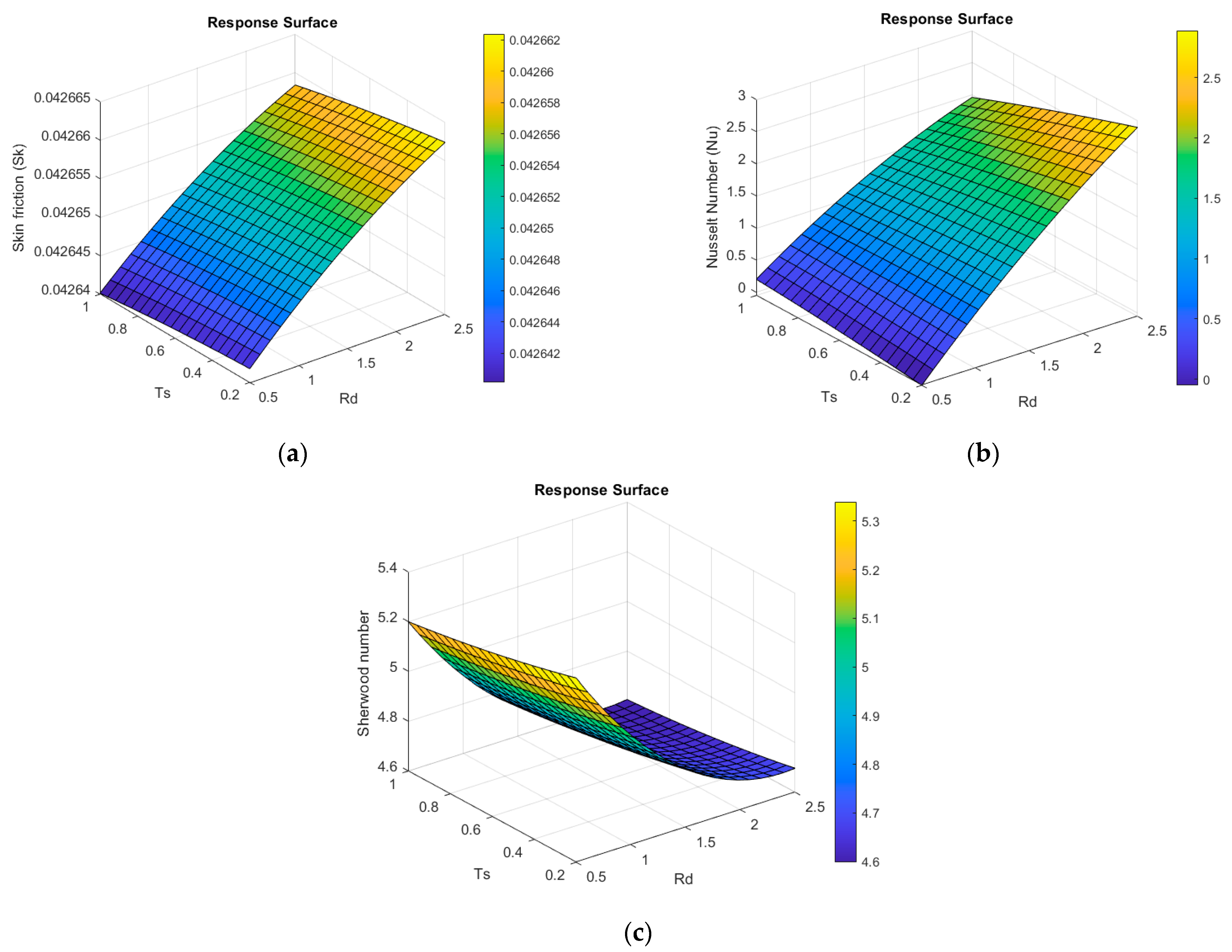
The used ranges of $Rd$, $Ts$, and $\gamma$ are $0.5\le Rd\le 2.5$, $0.2\le Ts\le 1.0$, and $0.3\le \gamma \le 1.5$. Here, the low values are $Rd=0.5,Ts=0.2$, and $\gamma =0.3$; the middle values are $Rd=1.5$, $Ts=0.5$, and $\gamma =0.8$, while the higher values are $Rd=2.5$, $Ts=1$, and $\gamma =1.5$. The current RSM model is presented in Figure 2 and

Table 2. Summary of the RSM model. Range of the parameters and their optimal values.

	Number of Observations	Error Degrees of Freedom	Root Mean Squared Error	R-Squared	Adjusted R-Squared	F-Statistic vs. Constant Model	p-Value
${\mathit{R}}_{\mathit{e}}^{{\displaystyle \frac{\mathbf{1}}{\mathbf{2}}}}{\mathit{C}}_{\mathit{f}}$	20	10	1.77 × 10−6	1	1	6.88 × 107	9.38 × 10−38
$\mathit{R}{\mathit{e}}^{{\displaystyle \frac{-\mathbf{1}}{\mathbf{2}}}}\mathit{N}\mathit{u}$	20	10	0.0428	0.999	0.998	1.04 × 103	1.2 × 10−13
${\displaystyle \frac{\mathbf{1}}{\sqrt{\mathit{R}\mathit{e}}}}\mathit{S}\mathit{h}$	20	10	0.0178	0.999	0.998	1.24 × 103	4.92 × 10−14
Parameter	Range	Optimal Value			Maximum Predicted value
		$R_e^{{\displaystyle \frac{1}{2}}}{C}_f$	$R{e}^{{\displaystyle \frac{-1}{2}}}Nu$	${\displaystyle \frac{1}{\sqrt{Re}}}Sh$	$R_e^{{\displaystyle \frac{1}{2}}}{C}_f$	$R{e}^{{\displaystyle \frac{-1}{2}}}Nu$	${\displaystyle \frac{1}{\sqrt{Re}}}Sh$
$\mathit{R}\mathit{d}$	$0.5\le Rd\le 2.5$	2.4465	2.5	0.5	0.042661	3.2683	6.3404
$\mathit{T}\mathit{s}$	$0.2\le Ts\le 1.0$	0.28362	0.2	0.2
$\mathit{\gamma }$	$0.3\le \gamma \le 1.5$	0.30001	1.5	1.4501

. The higher response in values of $R{e}^{{\displaystyle \frac{1}{2}}}{C}_f$ is noted at higher $Rd$, while the lower response of $R{e}^{{\displaystyle \frac{-1}{2}}}Nu$ is observed at $Ts=0.2$, while the higher values of $Ts$ gives higher responses in values of ${\displaystyle \frac{1}{\sqrt{Re}}}Sh$. Furthermore, Table 2 concludes that, for $R{e}^{{\displaystyle \frac{1}{2}}}{C}_f$, the optimal values of $Rd,Ts,\gamma$ are 2.4465, 0.28362, and 0.30001, respectively, and the maximum predicted value is $R{e}^{{\displaystyle \frac{1}{2}}}{C}_f=0.042661$. For $R{e}^{{\displaystyle \frac{-1}{2}}}Nu$, the optimal values of $Rd,Ts,\gamma$ are 2.5, 0.2, and 1.5, respectively, and the maximum predicted value is $R{e}^{{\displaystyle \frac{-1}{2}}}Nu=3.2683$. For ${\displaystyle \frac{1}{\sqrt{Re}}}Sh$, the optimal values of $Rd,Ts,\gamma$ are 0.5, 0.2, and 1.4501, respectively, and the maximum predicted value is ${\displaystyle \frac{1}{\sqrt{Re}}}Sh=6.3404$.

5. Results and Discussion

The effects of velocity slip, thermal radiation, and Dufour effects on the heterogeneous nanofluid flowing on the surface of a solid sphere in a porous material are examined, considering the impact of the first-order chemical reactive flowing. In addition, the influences of Stefan blowing and thermal jumping boundary constraints on the nanofluid are studied. The equations governing the model are converted into ordinary differential formulas employing similarity conversions. Additionally, neural network analysis was used to analyze and study the flow, temperature, and concentration of the nanofluid. All possible parameters’ effects on flow, temperature, and concentration are shown in Figure 3, Figure 4, Figure 5, Figure 6, Figure 7, Figure 8, Figure 9, Figure 10, Figure 11, Figure 12, Figure 13, Figure 14, Figure 15, Figure 16, Figure 17 and Figure 18. In addition, the effects of these factors on the surface frictional coefficient, Nusselt numbers, and Sherwood numbers are considered in

Table 3. Values of $\sqrt{Re}{C}_f$, $Nu/\sqrt{Re}$, and $Sh/\sqrt{Re}$ at $Ts=0.5$, $Sb=0.1$, $Ha=3$, $Nb=Nt=0.3$, $Mc=0.01$, $Nc=0.1$, $Nr=0.1$, and $Rd=0.5$.

${\mathit{L}}_1$	${\mathit{K}}_{\mathit{p}}$	${\mathit{\beta }}_{\mathit{k}}\times {10}^{-4}$	$\mathit{D}\mathit{u}$	$\mathit{\xi }$ = 0°			$\mathit{\xi }$ ≈ 30°
				$\sqrt{\mathit{R}\mathit{e}}{\mathit{C}}_{\mathit{f}}$	$\mathit{N}\mathit{u}/\sqrt{\mathit{R}\mathit{e}}$	$\mathit{S}\mathit{h}/\sqrt{\mathit{R}\mathit{e}}$	$\sqrt{\mathit{R}\mathit{e}}{\mathit{C}}_{\mathit{f}}$	$\mathit{N}\mathit{u}/\sqrt{\mathit{R}\mathit{e}}$	$\mathit{S}\mathit{h}/\sqrt{\mathit{R}\mathit{e}}$
0	0.2	0.1	0.01	0.06977698	0.03887837	3.707143	0.10592010	0.050480790	3.515093
0.2				0.04872854	0.07098851	4.924491	0.07434244	0.078014410	4.645483
0.4				0.03684446	0.09982599	5.465102	0.05642097	0.103610300	5.156902
0.6				0.02947896	0.12161520	5.760536	0.04525443	0.123497700	5.439749
0.8				0.02452222	0.13789410	5.944762	0.03770974	0.138583300	5.617456
1.0				0.02097446	0.15030550	6.070081	0.03229433	0.150201800	5.738942
0.2	0.2	0.1	0.01	0.04872854	0.07098851	4.924491	0.07434218	0.001429891	4.677425
	0.4			0.04929826	0.07024532	4.950215	0.07515649	0.000171984	4.699903
	0.6			0.04985042	0.06954124	4.974950	0.07594646	0.001043702	4.721559
	0.8			0.05038597	0.06887441	4.998767	0.07671350	0.002217169	4.742451
	1.0			0.05090591	0.06824173	5.021716	0.07745889	0.003340965	4.762618
	1.2			0.05141116	0.06763389	4.921647	0.07818382	0.004431233	4.782116
0.2	0.2	0.01	0.01	0.04864383	0.07086869	4.922597	0.07421168	0.001447275	4.674675
		0.04		0.04867213	0.07090594	4.923542	0.07425521	0.001441067	4.675590
		0.07		0.04870033	0.07094505	4.924491	0.07429872	0.001434858	4.676510
		0.10		0.04872854	0.07098851	4.925440	0.07434218	0.001429891	4.677425
		0.13		0.04875658	0.07102577	4.926390	0.07438557	0.001424303	4.678342
		0.16		0.04878458	0.07106550	4.921647	0.07442864	0.001421819	4.679263
0.2	0.2	0.1	0.001	0.04872950	0.22041360	4.857561	0.07434276	0.138431200	4.619795
			0.004	0.04872916	0.17111870	4.879892	0.07434252	0.093193110	4.639070
			0.007	0.04872881	0.12129860	4.902211	0.07434234	0.047514220	4.658291
			0.010	0.04872854	0.07098851	4.924491	0.07434218	0.001429890	4.677425
			0.013	0.04872820	0.02022522	4.946689	0.07434206	0.045005230	4.696422
			0.016	0.04872793	0.03092984	4.968755	0.07434195	0.091746450	4.715243

and

Table 4. Values of $\sqrt{Re}{C}_f$, $Nu/\sqrt{Re}$, and $Sh/\sqrt{Re}$ at $Kp=0.2$, $Ha=3$, $Nb=Nt=0.3$, $Mc=0.01$, $Du=0.001$, $Nc=0.1$, $Nr=0.1$, $L_1=0.5$, and ${\beta }_k=0.1\times {10}^{-4}$.

$\mathit{T}\mathit{s}$	$\mathit{S}\mathit{p}$	$\mathit{\gamma }$	$\mathit{R}\mathit{d}$	$\mathit{\xi }$ = 0°			$\mathit{\xi }$ ≈ 30°
				$\sqrt{\mathit{R}\mathit{e}}{\mathit{C}}_{\mathit{f}}$	${\mathit{N}}_{\mathit{u}}/\sqrt{\mathit{R}\mathit{e}}$	$\mathit{S}\mathit{h}/\sqrt{\mathit{R}\mathit{e}}$	$\sqrt{\mathit{R}\mathit{e}}{\mathit{C}}_{\mathit{f}}$	${\mathit{N}}_{\mathit{u}}/\sqrt{\mathit{R}\mathit{e}}$	$\mathit{S}\mathit{h}/\sqrt{\mathit{R}\mathit{e}}$
0.2	0.2	0.1	0.5	0.03276736	0.2080947	5.603502	0.05024611	0.1089331	5.330424
0.4				0.03276723	0.2865276	5.554257	0.05024545	0.1697553	5.295525
0.6				0.03276706	0.3399973	5.502920	0.05024471	0.2238794	5.254621
0.8				0.03276696	0.3757719	5.451360	0.05024422	0.2676373	5.210441
1.0				0.03276686	0.3983062	5.401159	0.05024375	0.3008638	5.165130
1.2				0.03276689	0.4107288	5.353595	0.05024346	0.3245187	5.120429
0.2	0.00			0.03289593	0.2832164	6.070204	0.05044355	0.17013090	5.783751
	0.05			0.03282977	0.2418788	5.834719	0.05034101	0.13647660	5.552588
	0.10			0.03276736	0.2080947	5.603502	0.05024611	0.10893310	5.330424
	0.15			0.03270887	0.1808442	5.378723	0.05015832	0.08654781	5.117743
	0.20			0.03265417	0.1590929	5.162140	0.05007688	0.06845159	4.914959
	0.25			0.03260312	0.1419081	4.954993	0.05000150	0.05390868	4.722321
0.2	0.2	0.0	0.5	0.03264627	0.1505862	5.295325	0.05006446	0.05994117	5.057343
		0.3		0.03267049	0.1772648	4.884532	0.05010321	0.08666392	4.617199
		0.6		0.03269696	0.2075794	4.437349	0.05014599	0.11707720	4.134715
		0.9		0.03272603	0.2417639	3.948381	0.05019335	0.15139950	3.603085
		1.2		0.03275821	0.2799947	3.411351	0.05024611	0.18974330	3.014307
		1.5		0.03279386	0.3223301	2.819007	0.05030523	0.23205330	2.359058
0.2	0.2	0.1	0.0	0.03264496	0.2987385	5.386341	0.05006721	0.32856760	5.116513
			0.5	0.03265417	0.1590929	5.162140	0.05007688	0.06845159	4.914959
			1.0	0.03266549	0.9344965	4.924056	0.05009235	0.79299910	4.684390
			1.5	0.03267317	1.7042140	4.775386	0.05010327	1.52531400	4.536570
			2.0	0.03267819	2.4235270	4.682597	0.05011062	2.21391900	4.442980
			2.5	0.03268168	3.0952270	4.621521	0.05011568	2.85833900	4.380822

.

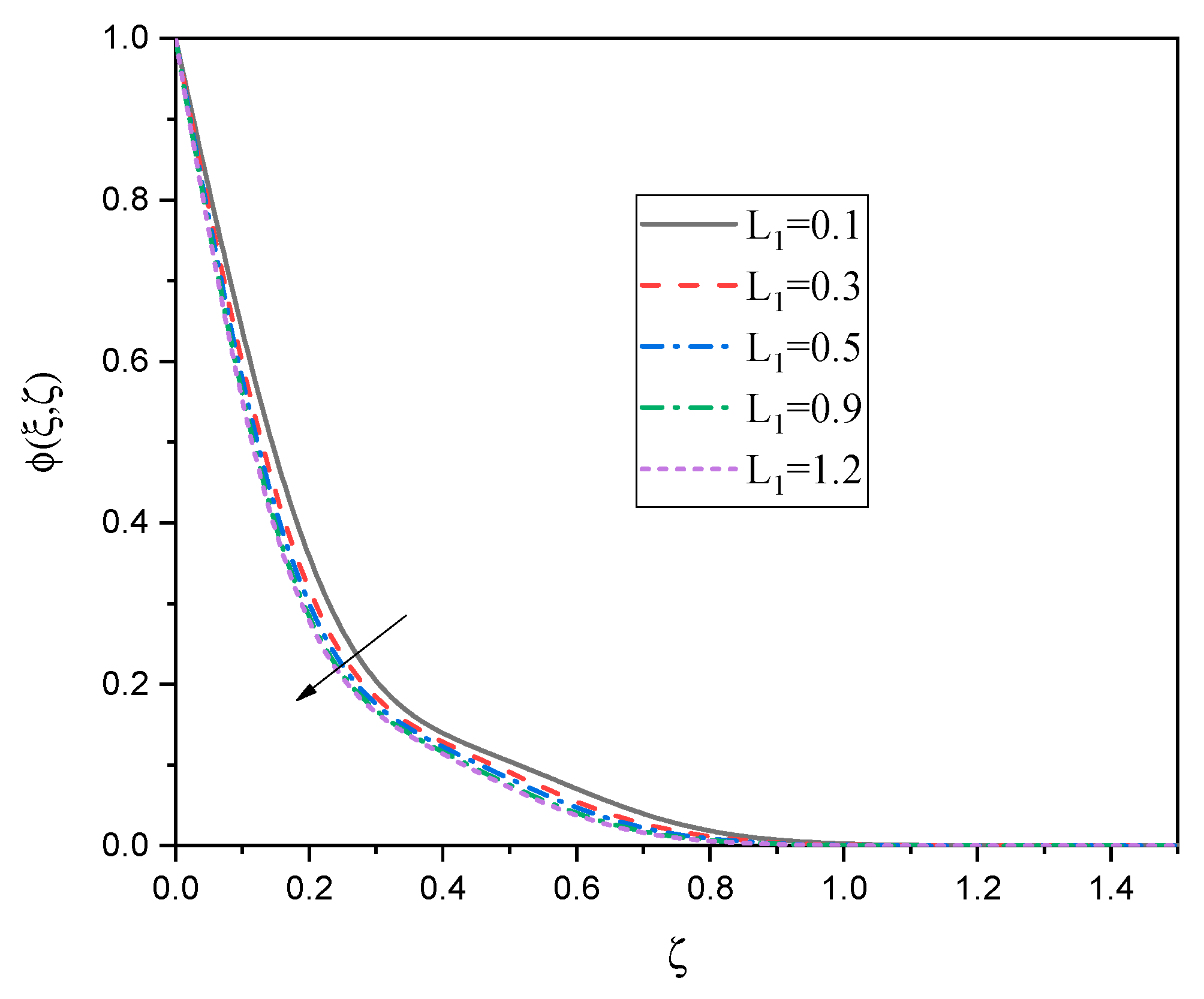
Figure 3, Figure 4 and Figure 5 study the relationships between the change in the velocity of the nanofluid $f_{\zeta }(\xi ,\zeta )$, its temperature $\theta \left(\xi ,\zeta \right)$, and its concentration $\varphi \left(\xi ,\zeta \right)$, and this is due to the change in the slippage parameter $L_1$ of the velocity, where we find that Figure 3 illustrates that the speed of the nanofluid $f_{\zeta }(\xi ,\zeta )$ upsurges with the rise in the values of the slippage parameter $L_1$ when $L_1$ takes the values of $L_1=0.1,0.3,0.5,0.9,1.2$, and then after that, the speed stabilizes after the value of $\zeta =1.5$ so that the speed is constant at a value of 1.4. The reason for this is that the slippage of the velocity causes an enhancement in the speed of the fluid because of the turbulent motion due to slippage of the molecules inside the nanofluid. Figure 4 indicates the drop in the temperature of the nanofluid $\theta \left(\xi ,\zeta \right)$ because of the growth in the slippage parameter of the velocity, where we find that the change is more evident away from the boundary layer. The physical reason for this is that when the slippage parameter improves, a higher heat transfer rate occurs, which causes a decline in temperature. Figure 5 establishes that because of improving the slippage parameter, there is a reduction in the concentration of the nanofluid $\varphi \left(\xi ,\zeta \right)$, which is less clear than its effect on temperatures $\theta \left(\xi ,\zeta \right)$. This effect occurs far from the boundary layer. The main reason for this is that the slippage velocity causes movement of the molecules that make up the nanofluid, which raises the distances between its molecules and reduces its concentration.

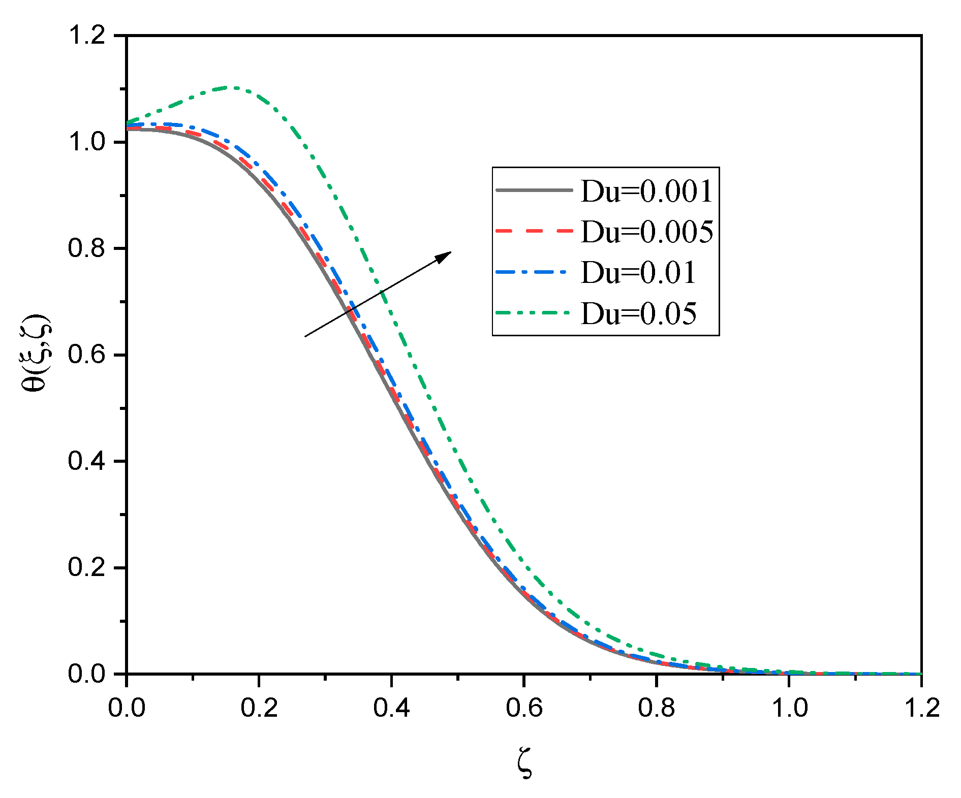
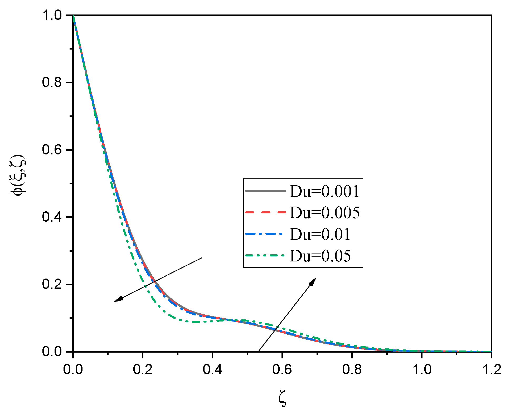
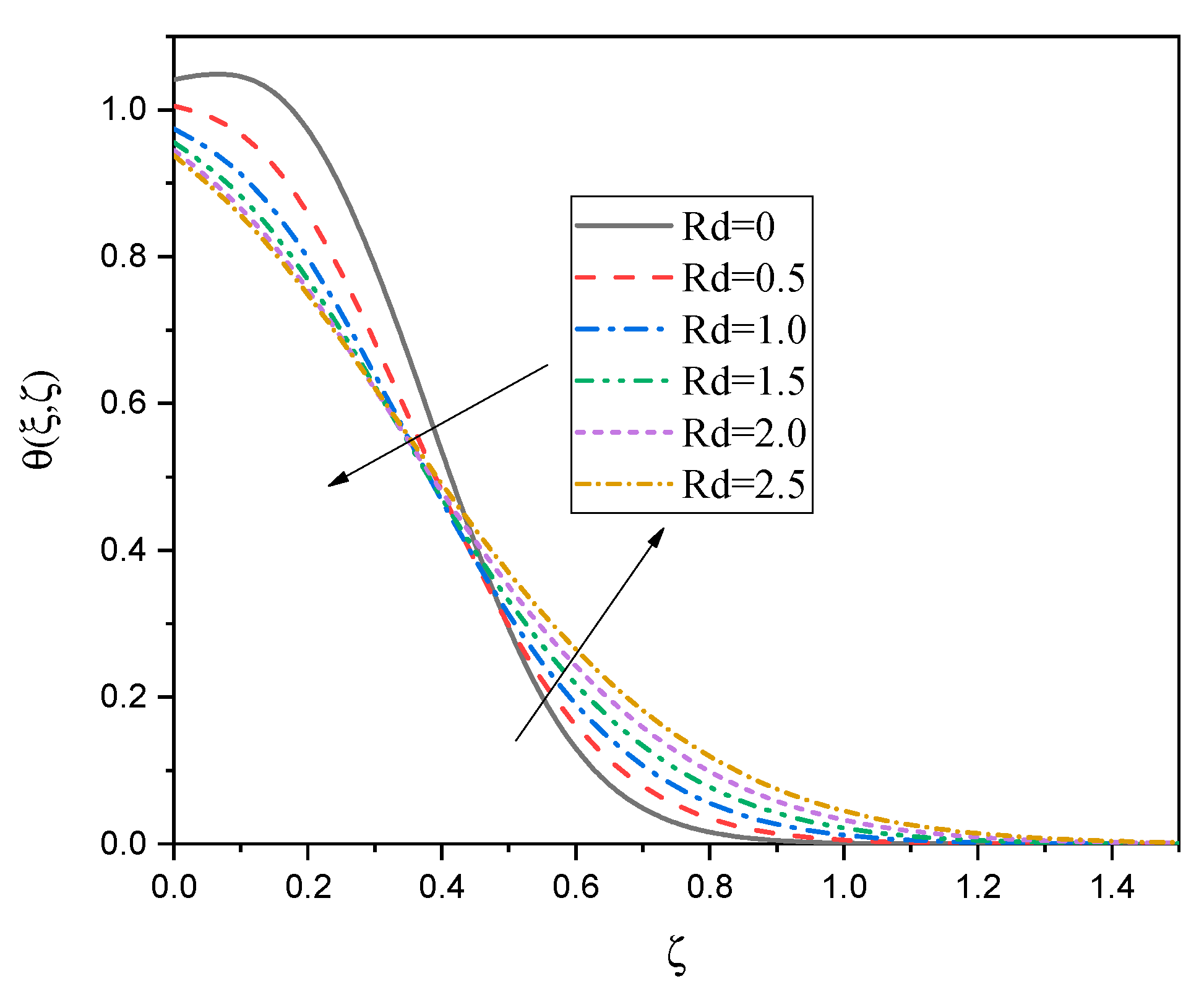
Figure 6 and Figure 7 show the nature of the relationship between the effect of Dufour ($Du=0.001,0.005,0.1,0.05$) and both the temperature $\theta \left(\xi ,\zeta \right)$ and concentration $\varphi \left(\xi ,\zeta \right)$ of the nanofluid. In Figure 6, we notice that increasing the effect of Dufour raises the temperature clearly near the boundary layer; then this increase begins to decrease as we move away from the boundary layer. Figure 7 explains that, when raising the effect of Dufour, the concentration of the nanofluid drops until the value of $\zeta =0.5$, and then it begins to rise after this value. The physical reason behind this is that the number of Dufour is directly proportional to the concentration difference $\left(C_w-C_{\infty }\right)$ and inversely proportional to the temperature difference $\left(T_w-T_{\infty }\right)$. Figure 8 displays the relationship between temperature $\theta \left(\xi ,\zeta \right)$ and the thermal radiation parameter $Rd$ of the nanofluid, as the figure indicates that the thermal radiation values range from 0 to 2.5. We can also notice that the higher the thermal radiation value, the lower the temperature value of the nanofluid as it approaches the boundary layer, and the farther away from it, the greater the temperature distribution inside the nanofluid with the upsurge in $Rd$ when $\zeta >0.4$. This can be explained physically as in this type of nanofluid. Thermal radiation plays an important role in controlling the temperature distribution due to stress moments, and when the thermal radiation parameter is equal to 0, i.e., in the absence of thermal radiation, the temperature is as high as possible near the boundary layer. This decrease at the boundary layer reflects the ability of the nanofluid to distribute heat more effectively, which contributes to improving the thermal properties of the nanofluid and makes it suitable for specific applications when it is desired to control temperatures. Figure 9 indicates the relationship between the concentration $\varphi \left(\xi ,\zeta \right)$ and the thermal radiation parameter $Rd$. It is noted that with the surge in the value of the thermal radiation parameter, we notice an upsurge in the concentration near the boundary layer until the value of $\zeta =0.4$. Then the concentration begins to decrease away from the boundary layer. It is noted that this behavior enhances the dispersion of nanoparticles and reduces their aggregation, which leads to a decrease in concentration due to the increase in dispersion. This phenomenon is important in applications that require precise control of the distribution of particles, as the figure illustrates that rising thermal radiation contributes to a more balanced distribution of nanoparticles.

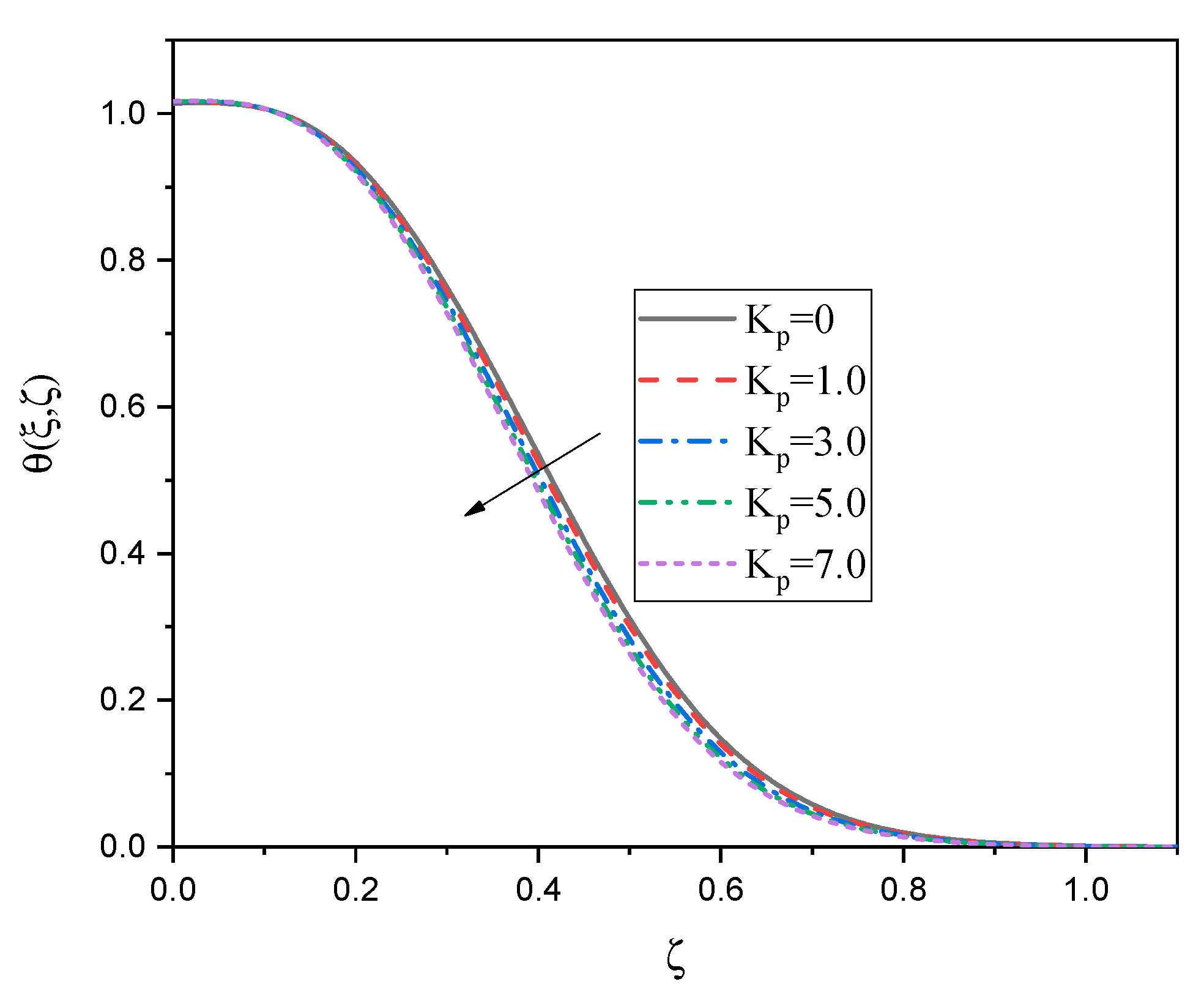
Figure 10 demonstrates the relationship between the dimensionless velocity $f_{\zeta }(\xi ,\zeta )$ and the porosity parameter $K_p$ of the nanofluid. It is noted that, with the increase in the porosity parameter $K_p=0,0.1,0.3,0.5,0.7$, the velocity of the nanofluid improves, and after $\zeta =1.5$, the velocity is stabilized. This indicates that the porous medium with higher porosity, i.e., higher values of the porosity parameter, allows faster passage of the nanofluid. This means that the more porous medium reduces the flow resistance and enhances the movement of the nanofluid. In this case, this property is useful in applications such as cooling and purification, where the flow efficiency can be improved, and the velocity can be controlled by modifying the porosity of the medium surrounding the nanofluid flow. Figure 11 displays the effect of the porosity parameter $K_p$ when $K_p=0,0.1,0.3,0.5,0.7$ on the temperature distribution of the nanofluid $\theta \left(\xi ,\zeta \right)$. It is noted that, when increasing the porosity parameter, the non-dimensional temperatures decrease significantly, especially in the middle of the nanofluid, indicating that the porous medium with high porosity enhances heat dissipation inside the nanofluid. This means that greater porosity leads to an improvement in heat transfer because of increasing the open area inside the medium, which allows heat to flow quickly away from the heat source. Physically, this behavior shows that the medium with high porosity improves the efficiency of cooling and heat transfer, which is important in thermal applications that require effective cooling, such as electronic devices and energy devices, where nanofluids are used to accelerate cooling and control temperatures. Here, we study the effect of the porosity parameter $K_p$ when $K_p=0,0.1,0.3,0.5,0.7$ on the distribution of nanofluid concentration $\varphi \left(\xi ,\zeta \right)$, as clearly shown in Figure 12. This figure illustrates that growing the porosity parameter leads to a reduction in the concentration of the nanofluid while increasing the distance $\zeta$, indicating that the medium with higher porosity facilitates the diffusion of nanoparticles away from the source physically. This means that high porosity provides larger and more permeable paths for the particles, which accelerates their dispersion and reduces their accumulation in a specific area. This effect is important in applications that require a regular distribution of nanoparticles, such as purification, filtration, and material transfer processes, as increasing porosity helps control the diffusion of the nanofluid and reduce its concentration in specific areas, which enhances the efficiency of the process and prevents the unwanted accumulation of these particles.

Figure 13 establishes the effect of the thermal slip factor $Ts$ on the temperature distributions of the nanofluid $\theta \left(\xi ,\zeta \right)$, where a noticeable boost in temperatures appears, especially near the boundary layer, which is the area in contact with the flow surface. This upsurge in temperatures is attributed to the effects of heat transfer and friction within the fluid, as the low thermal slip coefficient reduces the resistance to heat transfer, which helps and contributes to increasing heat transfer from the surface to the nanofluid. It is clear from this that there is a close relationship between the thermal slip coefficient and the behavior of temperatures, as temperatures increase when the thermal slip coefficient is as large as possible, which indicates the importance of choosing this coefficient in applications that require precise control of temperature distribution, such as cooling or heating systems in various engineering components.

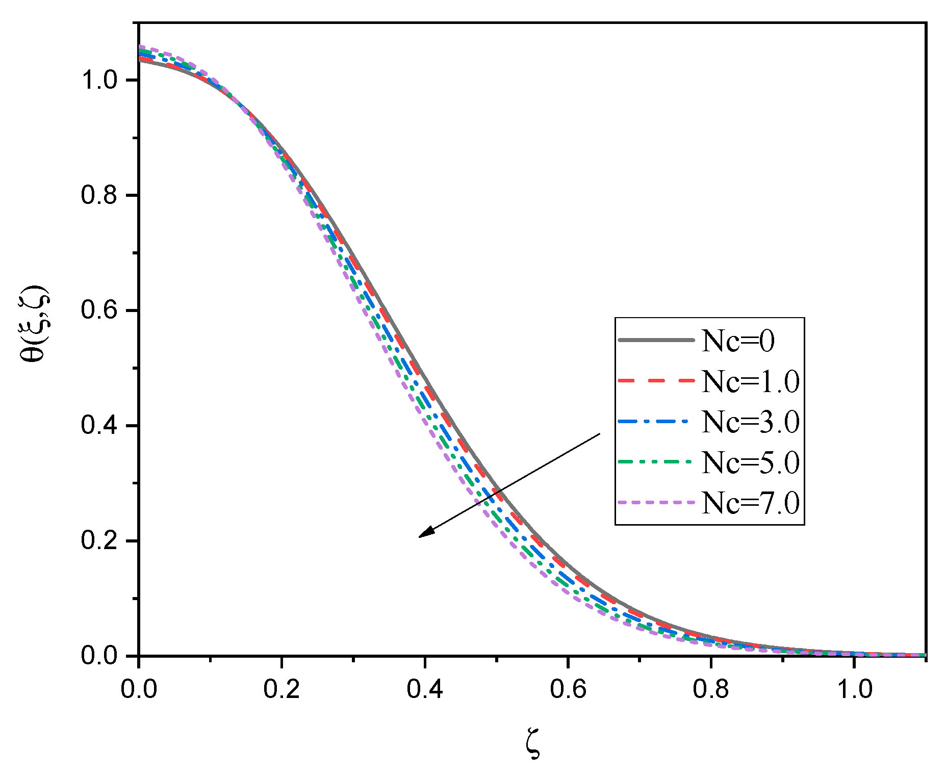
Figure 14 explains the effect of the nonlinear convective variable $Nc$ ($Nc=0,1.0,3.0,5.0,7.0)$ on the nanofluid velocity distribution $f_{\zeta }(\xi ,\zeta )$, where a significant improvement in velocity is observed near the boundary layer, which is the area in contact with the flow surface. This behavior is attributed to the effects of friction and pressure distribution inside the fluid, as the nonlinear convective variable leads to enhancing the rapid movement of molecules in this area, which contributes to a significant increase in velocity. After exceeding a value $\zeta =1.0$, velocity stability occurs, indicating that changes in the convective variable no longer affect velocity significantly. This behavior reflects the importance of understanding the relationship between the convective variable and fluid velocity in engineering applications, which in turn helps improve the efficiency and performance of heat transfer in advanced systems. To examine the effect of the nonlinear convective variable $Nc$ on the temperature distribution of the nanofluid $\theta \left(\xi ,\zeta \right)$, which is shown in Figure 15, it is noted that there is a slight increase in temperatures near the boundary layer, i.e., the surface in contact with the nanofluid. This initial improvement in temperatures is attributed to the transfer of heat from the surface to the nanofluid, as the nonlinear convective variable leads to an improvement in the efficiency of heat transfer in this region. However, after this slight increase, a general loss in temperatures occurs, indicating that the fluid begins to lose its heat because of dispersion and diffusion within the fluid. This physical behavior reflects the effect of changes in the nonlinear convection coefficient on the temperature distributions.

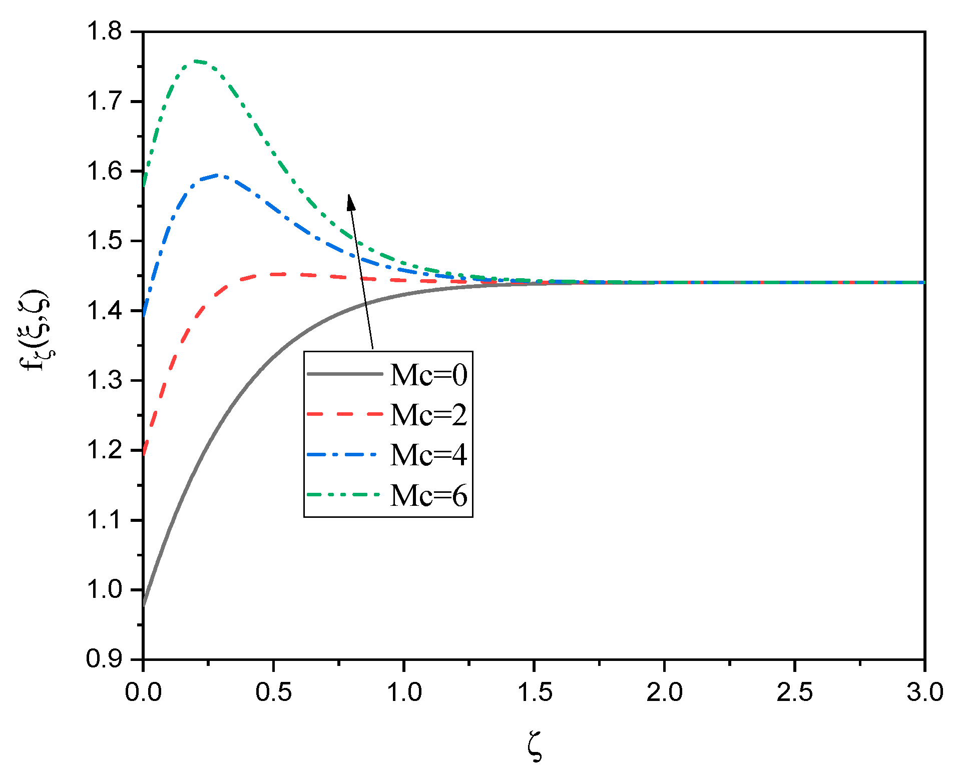
We can obtain the relationship between the mixed convective factor $Mc$ ($Mc=0,2,4,6$) and the nanofluid velocity distribution $f_{\zeta }(\xi ,\zeta )$ from Figure 16, where a large increase in velocity is observed near the flow surface, i.e., the boundary layer, which is the region adjacent to the nanofluid flow with the surface. This increase in velocity is attributed to the effects of friction and nanofluid pressure in this region, where the mixed convective factor enhances the movement of molecules, which in turn leads to a large increase in velocity after exceeding a certain value at one and a half; the velocity is fixed, which indicates that these changes in the mixed convective factor no longer significantly affect the velocity increase as is the case with the effect of the nonlinear convective variable. This behavior reflects the complex relationship between the fluid velocity and the mixed convective factor. Figure 17 displays the effect of the mixed convective factor $Mc$ on the temperature distribution of the nanofluid $\theta \left(\xi ,\zeta \right)$. A slight increase in temperature is observed near the boundary layer, which is the region adjacent to the flow surface. This initial increase in temperature is attributed to heat transfer from the surface to the fluid, where the mixed convective factor improves the efficiency of heat transfer in this region, thanks to the interactions of heat transfer and friction. However, after this slight increase, a noticeable decrease in temperature occurs as we move away from the boundary layer. This decrease indicates the loss of heat from the nanofluid because of dispersion and diffusion, which reflects the thermodynamic effects that affect the behavior of temperatures, which illustrates the relationship between the mixed convective factor and temperatures through this figure.

Figure 18 displays the extent of the relationship between the chemical reactive coefficient $\gamma$ for $\gamma =0,0.5,1.0,1.5$ and the concentration distribution of the nanofluid $\varphi \left(\xi ,\zeta \right)$, where a rapid decrease in concentration is observed because of the increase in the chemical reactive coefficient. This reduction is clear when moving away from the boundary layer, i.e., in the center of the nanofluid. This behavior is because chemical reactions occur inside the nanofluid, where the chemical reaction coefficient directly affects the speed of these reactions. The increase in the reaction coefficient leads to an acceleration in the consumption of reactants and the production of products, which causes a significant decrease in the concentration of the nanofluid in the center of the fluid. This decrease indicates that transport and mixing reactions play a crucial role in the concentration distribution, which affects and is reflected in thermodynamics and fluid mechanics on the behavior of the fluid. This effect highlights the importance of studying chemical reactions in engineering applications and chemical processing systems, as this phenomenon can affect the efficiency of processes and reduce material losses.

Table 3 examines the effects of slippage velocity $L_1$, porosity parameter $K_p$, couple stress parameter ${\beta }_k$, and Dufour number $Du$ on surface frictional factor $\sqrt{Re}{C}_f$, heat $Nu/\sqrt{Re}$, and mass $Sh/\sqrt{Re}$ transfers rate at $\xi$ = 0° and $\xi$ = 30°. It is noted from Table 3 that the parameters of porosity $K_p$ and the couple stress parameter ${\beta }_k$ increase the surface frictional factor, in complete contrast to the parameters of velocity slippage $L_1$ and the Dufour number $Du$. It can also be noted that the rates of heat transfer upsurge with the rise in the parameters of $L_1$ and ${\beta }_k$, while it reduces with the parameters of $K_p$ and $Du$. Meanwhile, the mass transfer rates rise with growth in all parameters. Table 4 displays the influences of Stefan number $Sp$, chemical reactive factor $\gamma$, and thermal radiative parameter $Rd$ on surface frictional factor $\sqrt{Re}{C}_f$, heat $Nu/\sqrt{Re}$, and mass $Sh/\sqrt{Re}$ transfer rate at $\xi$ = 0° and $\xi$ = 30°. It is noted from Table 4 that the surface frictional factor upsurges with the rise of both $\gamma$ and $Rd$, while the opposite occurs when the values of $Ts$ and $Sp$ increase. When studying the heat transfer rates, we find that $Ts$, $\gamma$, and $Rd$ increase the heat transfer rates, while the opposite occurs with $Sp$, while all the parameters in this table work to reduce the mass transfer rates of the nanofluid when their values upsurge. Here, it should be mentioned that the fluid temperature is deviated from the boundary temperature due to the thermal slip. Therefore, for all values of $\xi$, the thickness of the thermal boundary layer is reduced, resulting in an improvement in the convective heat transfer.

6. ANN Analyses

The training model of ANN (Figure 19) that is presented by Levenberg–Marquardt is used in this section for three implemented variables. These variables are the Dufour number $Du$, the slippage velocity $L_1$, and the thermal slippage parameter $Ts$. These parameters are compared with the values of the Nusselt number at $\xi$ = 0°. In addition, the following is the mathematical formula for the Mean Square Error ($MSE$), the metrics for the Coefficient of Determination ($R$), and the errors that occur between the values that were forecasted and those that were really achieved:

$$MSE={\displaystyle \frac{1}{N}}{\sum }_{i=1}^N{\left(X_{\mathit{exp}(i)}-X_{ANN\left(i\right)}\right)}^2,R=\sqrt{1-{\displaystyle \frac{{\sum }_{i=1}^N{\left(X_{\mathit{exp}(i)}-X_{ANN\left(i\right)}\right)}^2}{{\sum }_{i=1}^N{\left(X_{\mathit{exp}(i)}\right)}^2}}},$$

$$ErrorRate(\%)=\left[{\displaystyle \frac{{XANN}_{exp}}{X_{exp}}}\times 100\right]$$

A custom MATLAB code was developed to analyze the data using Artificial Neural Network (ANN) techniques. The ANN model was trained using a dataset imported from Excel files, which were generated from the FDM-based MATLAB code. The input features ($Du,L_1,Ts$) and the target output (Nu) were extracted for model training. The dataset consisted of 450 values; those were divided into 70% training, 15% validation, and 15% testing using the dividerand function. A single hidden layer with 10 neurons was employed, and the network was implemented using MATLAB’s fitnet function. The Levenberg–Marquardt (trainlm) optimization algorithm, the default for fitnet, was used to minimize the error. The activation functions were tansig (hyperbolic tangent sigmoid) in the hidden layer and purelin (linear) in the output layer. The network was trained for up to 1000 epochs, with a performance goal of 1 × 10⁻⁶. Model performance was evaluated using Mean Squared Error (MSE), ensuring robust validation.

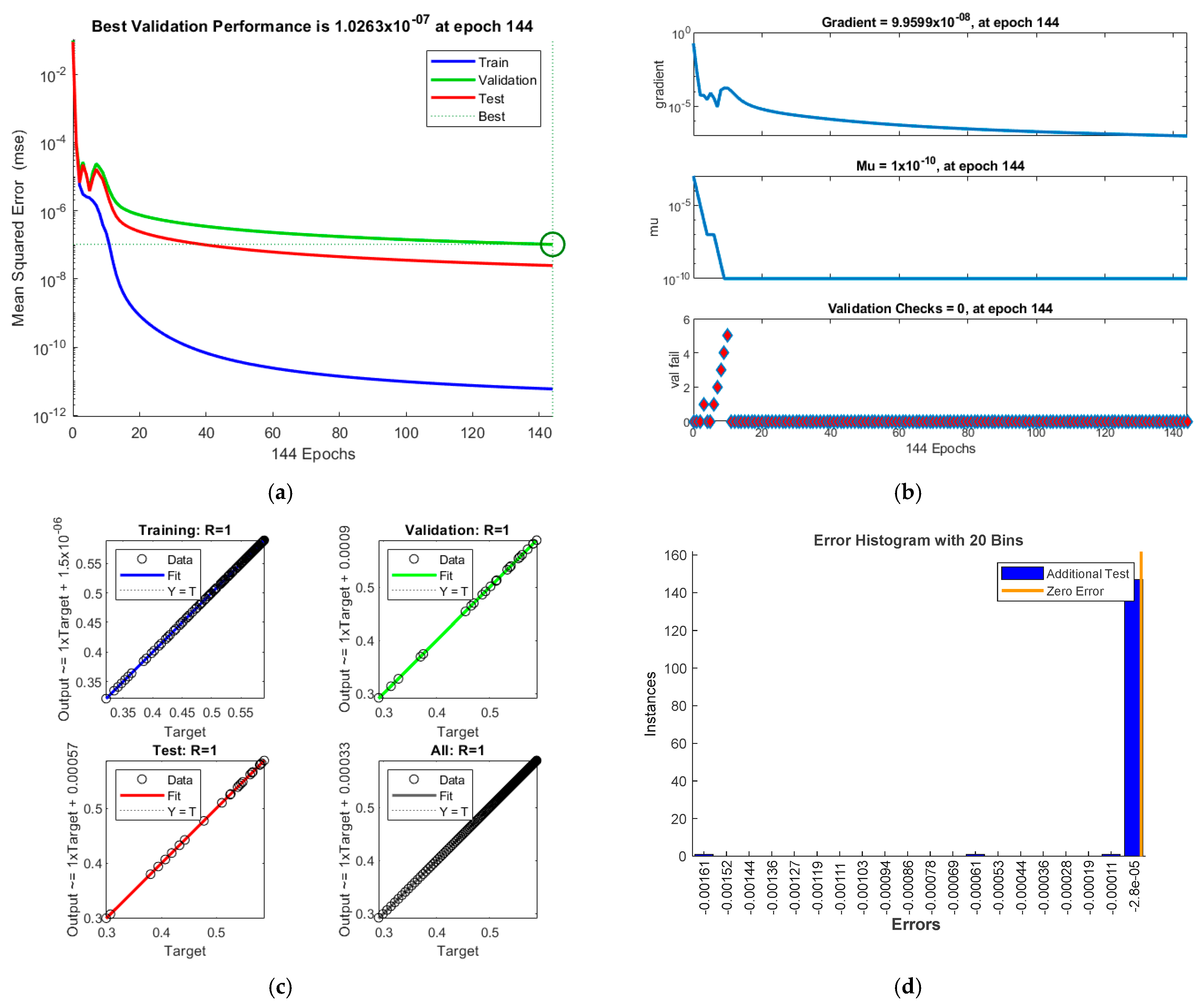
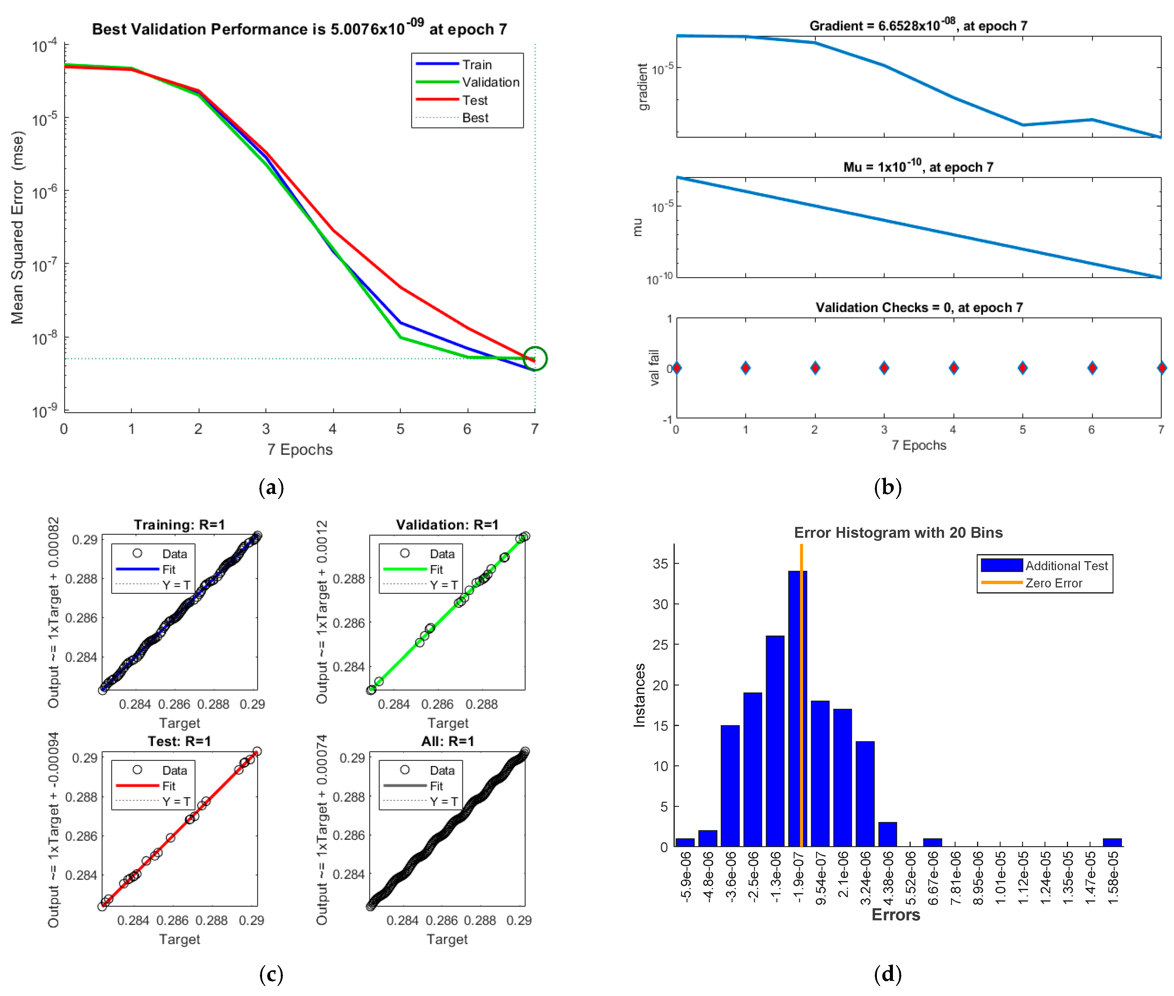
Figure 20a–d illustrate the MSE values; the efficiency in the structure of “gradients”, the control parameter “mu”, and the “validation check” of the backpropagation algorithm, as well as the regression diagram and the error histogram, are displayed for the Nusselt number in relation to the changes of the Dufour number $Du$. It is worth noting that the best validation performance is 3.6245 × 10⁻¹² at epoch 76. The gradient is equal to 9.8756 × 10⁻⁸, mu = 1 × 10⁻¹², and the validation check is equal to 3 at epoch 79. Additionally, the goal value of $R=1$. Furthermore, the differences between the predicted and target values for each dataset demonstrate that the disparities between the target and estimated values from the ANN model are minor, with errors clustering around the zero-error line. This is demonstrated by the similarities between the two sets of values. Based on this, it seems that the training procedure was finished with a minimal number of mistakes. In the same context, Figure 21a–d depict the tools that were stated before for the second parameter, which is the slipping velocity $L_1$. It has been shown that the optimal validation performance was 1.0263 × 10⁻⁷ at epoch 144. Additionally, the gradient was equal to 9.9599 × 10⁻⁸, mu = 1 × 10⁻¹⁰, and the validation check was equal to zero at epoch 144. Furthermore, the goal value of $R=1$. Additionally, the differences between the target values and the anticipated values are quite tiny, and the error line is getting closer and closer to zero. In addition, Figure 22 shows that the validation curve appears to be overfitting, and this is due to the fact that the model is trained for too many iterations; it may start fitting noise in the training data, leading to a widening gap between training and validation performance. Furthermore, for the third parameter (thermal slippage parameter $Ts$), Figure 22a–d exhibit the ANN training and tests for the average $Nu$ values. It revealed that the best authorization execution is $5.0076\times {10}^{-9}$ at epoch 7, the gradient is equal to $6.6528\times {10}^{-8}$, mu = $1\times {10}^{-10}$, the authorization check = 0 at epoch 7, and the target value of $R=1$. All these observations show the best-fit model for the proposed factors and indicate successful training with minimal errors.

7. Concluding Remarks

Computational simulations of the couple stress nanofluid flow in the presence of diffusion thermo-effect over a solid sphere that is embedded in a porous medium have been carried out. Various significant effects have been considered, such as second-order slip conditions, Stefan blowing, convective boundary conditions, thermal slip conditions, exponential chemical reactions, thermal radiation, and heat internal heat generation. Non-similar transformations were used to convert the governing system to a non-similar form, and effective finite difference approaches were applied. The effective artificial neural network techniques were proposed to predict some important physical parameters, such as the Nusselt number, under the influence of some major factors, such as the Du number, velocity, and thermal slip parameters. The following major outcomes can be summarized:

• The couple stress parameter causes an improvement in the gradients of the velocity, temperature, and concentration, and hence the skin friction. The values of the Nusselt number and Sherwood number increase significantly.
• A clear enhancement in the nanofluid temperature is obtained as the Dufour number is altered, while the heat transfer rate is decreasing.
• The slippage parameter in the case of the couple stress nanofluid flow gives higher velocity features, while both the temperature and concentration are reduced.
• For all values of $\xi (\xi$ = 0°, $\xi$ ≈ 30°) the thermal slip factor $Ts$ gives higher heat transfer rates.
• Good target values using ANN are obtained for all considered parameters, where R = 1.
• The mixed convection parameter causes the nanofluid velocity to increase significantly near the boundary layer due to friction and nanofluid pressure.
• The heat transfer from the sphere surface causes a slight temperature rise occurring near the boundary layer, but as distance increases, the temperature decreases due to heat dispersion and diffusion.

References

1. Brunton, S.L.; Noack, B.R.; Koumoutsakos, P. Machine learning for fluid mechanics. Annu. Rev. Fluid Mech. 2020, 52, 477–508. [Google Scholar]
2. Vinuesa, R.; Brunton, S.L.; McKeon, B.J. The transformative potential of machine learning for experiments in fluid mechanics. Nat. Rev. Phys. 2023, 5, 536–545. [Google Scholar] [CrossRef]
3. Duraisamy, K.; Iaccarino, G.; Xiao, H. Turbulence modeling in the age of data. Annu. Rev. Fluid Mech. 2019, 51, 357–377. [Google Scholar]
4. Ling, J.; Kurzawski, A.; Templeton, J. Reynolds averaged turbulence modelling using deep neural networks with embedded invariance. J. Fluid Mech. 2016, 807, 155–166. [Google Scholar]
5. Morimoto, M.; Fukami, K.; Zhang, K.; Nair, A.G.; Fukagata, K. Convolutional neural networks for fluid flow analysis: Toward effective metamodeling and low dimensionalization. Theor. Comput. Fluid Dyn. 2021, 35, 633–658. [Google Scholar]
6. Rabault, J.; Kuchta, M.; Jensen, A.; Réglade, U.; Cerardi, N. Artificial neural networks trained through deep reinforcement learning discover control strategies for active flow control. J. Fluid Mech. 2019, 865, 281–302. [Google Scholar]
7. Zhang, Y.; Zhang, D.; Jiang, H. Review of challenges and opportunities in turbulence modeling: A comparative analysis of data-driven machine learning approaches. J. Mar. Sci. Eng. 2023, 11, 1440. [Google Scholar] [CrossRef]
8. Jubair, S.; Ali, B.; Siddiqui, M.I.H. Neural network-based thermal analysis of stratified nanostructured materials with couple-stress nanofluid flow and gyrotactic microorganisms under exponential heating/cooling conditions. Mod. Phys. Lett. B 2024, 39, 2450438. [Google Scholar] [CrossRef]
9. Jan, A.; Mushtaq, M.; Khan, M.I.; Farooq, U. Integrated artificial intelligence and non-similar analysis for forced convection of radially magnetized ternary hybrid nanofluid of Carreau-Yasuda fluid model over a curved stretching surface. Int. J. Numer. Methods Fluids 2024, 96, 1864–1882. [Google Scholar] [CrossRef]
10. Rehman, K.U.; Shatanawi, W.; Alharbi, W.G.; Shatnawi, T.A. AI-Neural Networking Analysis (NNA) of Thermally Slip Magnetized Williamson (TSMW) fluid flow with heat source. Case Stud. Therm. Eng. 2024, 56, 104248. [Google Scholar]
11. Swamy, H.K.; Ryu, D.; Kim, H.; Sankar, M.; Do, Y. Exploring bioconvection dynamics within an inclined porous annulus: Integration of CFD and AI on the synergistic effects of hybrid nanofluids, oxytactic microorganisms, and magnetic field. Int. Commun. Heat Mass Transf. 2024, 159, 107999. [Google Scholar] [CrossRef]
12. Akbar, N.S.; Zamir, T.; Noor, T.; Muhammad, T.; Ali, M.R. Heat transfer enhancement using ternary hybrid nanofluid for cross-viscosity model with intelligent Levenberg-Marquardt neural networks approach incorporating entropy generation. Case Stud. Therm. Eng. 2024, 63, 105290. [Google Scholar] [CrossRef]
13. Babu, D.H.; Naidu, K.K.; Babu, B.H.; Raju, K.V.; Reddy, S.H.; Narayana, P.S. Numerical and neural network approaches to heat transfer flow in MHD dissipative ternary fluid through Darcy-Forchheimer permeable channel. Case Stud. Therm. Eng. 2024, 60, 104777. [Google Scholar] [CrossRef]
14. Khan, Z.; Thabet, E.N.; Abd-Alla, A.; Elhag, S. Artificial neural networks (ANNs) in an Electroosmosis-Controlled Darcy-Forchheimer flow for the Casson nanofluid model over stretching sheet. Int. J. Heat Fluid Flow 2024, 109, 109507. [Google Scholar] [CrossRef]
15. Alotaibi, A.; Gul, T.; Alotaibi, I.M.S.; Alghuried, A.; Alshomrani, A.S.; Alghuson, M. Artificial neural network analysis of the flow of nanofluids in a variable porous gap between two inclined cylinders for solar applications. Eng. Appl. Comput. Fluid Mech. 2024, 18, 2343418. [Google Scholar] [CrossRef]
16. Rehman, K.U.; Shatanawi, W.; Çolak, A.B. Neural networking-based analysis of heat transfer in MHD thermally slip Carreau fluid flow with heat generation. Case Stud. Therm. Eng. 2024, 54, 103995. [Google Scholar] [CrossRef]
17. Shilpa, B.; Leela, V.; Badruddin, I.A.; Kamangar, S.; Bashir, M.N.; Ali, M.M. Integrated Neural Network based Simulation of Thermo Solutal Radiative Double-Diffusive Convection of Ternary Hybrid Nanofluid Flow in an Inclined Annulus with Thermophoretic Particle Deposition. Case Stud. Therm. Eng. 2024, 62, 105158. [Google Scholar] [CrossRef]
18. Khan, W.; Pop, I. Boundary-layer flow of a nanofluid past a stretching sheet. Int. J. Heat Mass Transf. 2010, 53, 2477–2483. [Google Scholar] [CrossRef]
19. Makinde, O.D.; Aziz, A. Boundary layer flow of a nanofluid past a stretching sheet with a convective boundary condition. Int. J. Therm. Sci. 2011, 50, 1326–1332. [Google Scholar] [CrossRef]
20. Buongiorno, J. Convective transport in nanofluids. J. Heat Transfer. Mar. 2006, 128, 240–250. [Google Scholar] [CrossRef]
21. Bhattacharyya, K.; Layek, G. Magnetohydrodynamic boundary layer flow of nanofluid over an exponentially stretching permeable sheet. Phys. Res. Int. 2014, 2014, 592536. [Google Scholar]
22. Kakaç, S.; Pramuanjaroenkij, A. Review of convective heat transfer enhancement with nanofluids. Int. J. Heat Mass Transf. 2009, 52, 3187–3196. [Google Scholar] [CrossRef]
23. Saidur, R.; Leong, K.; Mohammed, H.A. A review on applications and challenges of nanofluids. Renew. Sustain. Energy Rev. 2011, 15, 1646–1668. [Google Scholar]
24. Rehman, A.; Inc, M.; Tawfiq, F.M.; Bilal, M. Analytical analysis of 2D couple stress flow of blood base nanofluids with the influence of viscous dissipation over a stretching surface. Mod. Phys. Lett. B 2024, 39, 2450446. [Google Scholar] [CrossRef]
25. Aljaloud, A.S.; Manai, L.; Tlili, I. Flow of couple stress nanofluid due to stretching surface with applications of induced magnetic field and variable thermal conductivity. Case Stud. Therm. Eng. 2024, 57, 104356. [Google Scholar]
26. Li, S.; Bilal, M.; Mir, A.; Kolsi, L.; Muhammad, T.; Ahmad, Z. Parametric simulation of couple-stress nanofluid flow subject to thermal and solutal time relaxation factors. J. Therm. Anal. Calorim. 2024, 1–14. [Google Scholar] [CrossRef]
27. Dasari, R.; Kumar, N.N.; Basha, H. Lorentz force influenced entropy generation in couple stress squeezed hybrid-nanofluid flow: Application to cardiovascular hemodynamics. Numer. Heat Transf. Part B Fundam. 2024, 85, 1254–1286. [Google Scholar] [CrossRef]
28. Kathyayani, G.; Rao, S.S.N. Influence of couple stress, radiation, and activation energy on MHD flow and entropy generation in Maxwell hybrid nanofluid flow over a flat plate, Proceedings of the Institution of Mechanical Engineers. Part E J. Process Mech. Eng. 2024, 09544089241286741. [Google Scholar] [CrossRef]
29. Rana, P.; Gupta, S.; Gupta, G. Optimization of heat transfer by nonlinear thermal convection flow past a solid sphere with Stefan blowing and thermal slip using Taguchi method. Int. Commun. Heat Mass Transf. 2023, 141, 106580. [Google Scholar] [CrossRef]
30. Al-hanaya, A.; Rashed, Z.; Ahmed, S.E. MHD Casson flow over a solid sphere surrounded by porous material in the presence of Stefan blowing and slip conditions. Alex. Eng. J. 2024, 103, 402–412. [Google Scholar]
Figure 1. Flow system diagram.
Processes 13 01055 g001
Figure 2. Plot of a 2D slice of the response surface for (a) skin frictions, (b) Nusselt number, and (c) Sherwood number.
Processes 13 01055 g002
Figure 3. Behaviors of f ζ ( ξ , ζ ) with the variations of L 1 at T s = 0.1 , N b = N t = 0.2 , M c = 0.01 , D u = 0.01 , N c = N r = 0.1 , R d = 0.1 , and β k = 0.1 × 10 4 .
Processes 13 01055 g003
Figure 4. Profiles of θ ξ , ζ with the variations of L 1 at T s = 0.1 , N b = N t = 0.2 , M c = 0.01 , D u = 0.01 , N c = N r = 0.1 , R d = 0.1 , and β k = 0.1 × 10 4 .
Processes 13 01055 g004
Figure 5. Behaviors of ϕ ξ , ζ with the variations of L 1 at T s = 0.1 , N b = N t = 0.2 , M c = 0.01 , D u = 0.01 , N c = N r = 0.1 , R d = 0.1 , and β k = 0.1 × 10 4 .
Processes 13 01055 g005
Figure 6. Profiles of θ ( ξ , ζ ) with the variations of D u at T s = 0.1 , N b = N t = 0.3 , M c = 0.01 , L 1 = 0.5 , N c = N r = 0.1 , R d = 0.1 , and β k = 0.1 × 10 4 .
Processes 13 01055 g006
Figure 7. Profiles of ϕ ( ξ , ζ ) with the variations of D u at T s = 0.1 , N b = N t = 0.3 , M c = 0.01 , L 1 = 0.5 , N c = N r = 0.1 , R d = 0.1 , and β k = 0.1 × 10 4 .
Processes 13 01055 g007
Figure 8. Profiles of θ ( ξ , ζ ) with the variations of R d at T s = 0.1 , K p = 0.5 , N b = N t = 0.3 , M c = 0.01 , L 1 = 0.8 , N c = N r = 0.1 , D u = 0.01 , and β k = 0.1 × 10 4 .
Processes 13 01055 g008
Figure 9. Profiles of ϕ ( ξ , ζ ) with the variations of R d at T s = 0.1 , K p = 0.5 , N b = N t = 0.3 , M c = 0.01 , L 1 = 0.8 , N c = N r = 0.1 , D u = 0.01 , and β k = 0.1 × 10 4 .
Processes 13 01055 g009
Figure 10. Behaviors of f ζ ( ξ , ζ ) with the variations of K p at T s = 0.1 , N b = N t = 0.3 , H a = 3 , M c = 0.01 , D u = 0.01 , N c = N r = 0.1 , R d = 0.1 , L 1 = 0.5 , and β k = 0.1 × 10 4 .
Processes 13 01055 g010
Figure 11. Profiles of θ ( ξ , ζ ) with the variations of K p at T s = 0.1 , N b = N t = 0.3 , H a = 3 , M c = 0.01 , D u = 0.01 , N c = N r = 0.1 , R d = 0.1 , L 1 = 0.5 , and β k = 0.1 × 10 4 .
Processes 13 01055 g011
Figure 12. Profiles of ϕ ( ξ , ζ ) with the variations of K p at T s = 0.1 , N b = N t = 0.3 , H a = 3 , M c = 0.01 , D u = 0.01 , N c = N r = 0.1 , R d = 0.1 , L 1 = 0.5 , and β k = 0.1 × 10 4 .
Processes 13 01055 g012
Figure 13. Profiles of θ ( ξ , ζ ) with the variations of T s at K p = 0.5 , N b = N t = 0.3 , H a = 3 , M c = 0.01 , D u = 0.01 , N c = N r = 0.1 , R d = 0.5 , L 1 = 0.8 , and β k = 0.1 × 10 4 .
Processes 13 01055 g013
Figure 14. Behaviors of f ζ ( ξ , ζ ) with the variations of N c at T s = 0.5 , H a = 3 , N b = N t = 0.3 , M c = 0.01 , D u = 0.01 , M c = 1 , N r = 0.1 , R d = 0.5 , L 1 = 0.8 , and β k = 0.1 × 10 4 .
Processes 13 01055 g014
Figure 15. Profiles of θ ( ξ , ζ ) with the variations of N c at T s = 0.5 , H a = 3 , N b = N t = 0.3 , M c = 0.01 , D u = 0.01 , M c = 1 , N r = 0.1 , R d = 0.5 , L 1 = 0.8 , and β k = 0.1 × 10 4 .
Processes 13 01055 g015
Figure 16. Behaviors of f ζ ( ξ , ζ ) with the variations of M c at T s = 0.5 , H a = 3 , N b = N t = 0.3 , M c = 0.01 , D u = 0.01 , N c = 1 , N r = 0.1 , R d = 0.5 , L 1 = 0.8 , and β k = 0.1 × 10 4 .
Processes 13 01055 g016
Figure 17. Profiles of θ ( ξ , ζ ) with the variations of M c at T s = 0.5 , H a = 3 , N b = N t = 0.3 , M c = 0.01 , D u = 0.01 , N c = 1 , N r = 0.1 , R d = 0.5 , L 1 = 0.8 , and β k = 0.1 × 10 4 .
Processes 13 01055 g017
Figure 18. Profiles of ϕ ( ξ , ζ ) with the variations of γ at T s = 0.1 , S p = 0.1 , K p = 0.5 , H a = 3 ,   N b = N t = 0.3 , M c = 0.01 , D u = 0.01 , N c = 0.1 , N r = 0.1 , R d = 0.1 , L 1 = 0.5 , and β k = 0.1 × 10 4 .
Processes 13 01055 g018
Figure 19. Neural Network Architecture.
Processes 13 01055 g019
Figure 20. (a) MSE values for parameter D u . (b) Performance in the form of “gradients”, control parameter “mu”, and “validation check” of the backpropagation algorithm for parameter D u . (c) Regression illustration for D u . (d) The variations between the predicted and target values for each dataset for D u .
Processes 13 01055 g020
Figure 21. (a) MSE values for parameter L 1 . (b) Performance in the form of “gradients”, control parameter “mu”, and “validation check” of the backpropagation algorithm for parameter L 1 . (c) Regression diagram for L 1 . (d) The variations between the predicted and target values for each dataset for L 1 .
Processes 13 01055 g021
Figure 22. (a) MSE values for parameter T s . (b) Performance in the form of “gradients”, control parameter “mu”, and “validation check” of the backpropagation algorithm for parameter T s . (c) Regression diagram for parameter T s . (d) The differences between the predicted and target values for each dataset for T s .
Processes 13 01055 g022