
Experimental Study of Dye Degradation in a Single-Jet Cavitation System


Abstract
:1. Introduction
2. Configuration
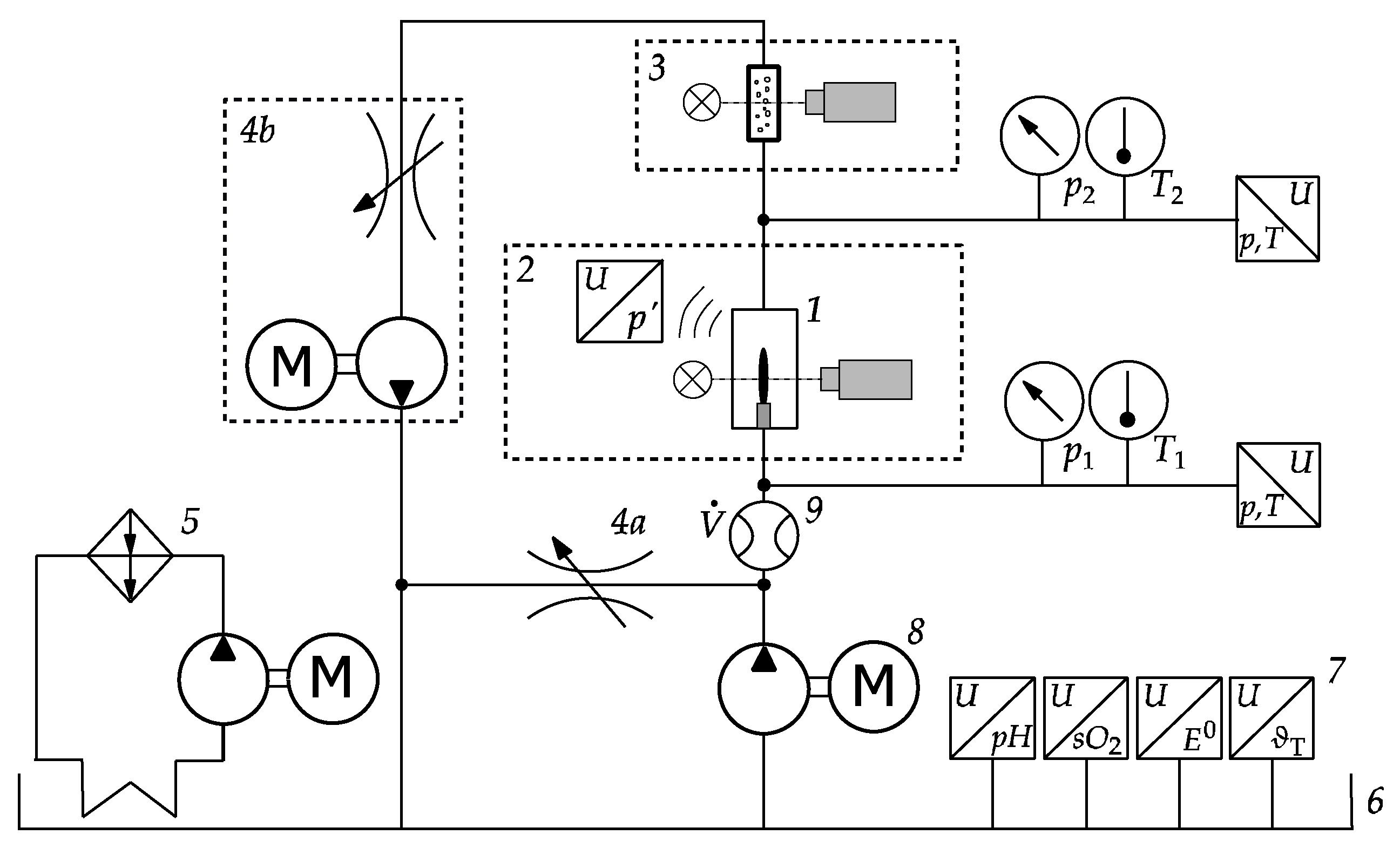
2.1. Experimental Setup

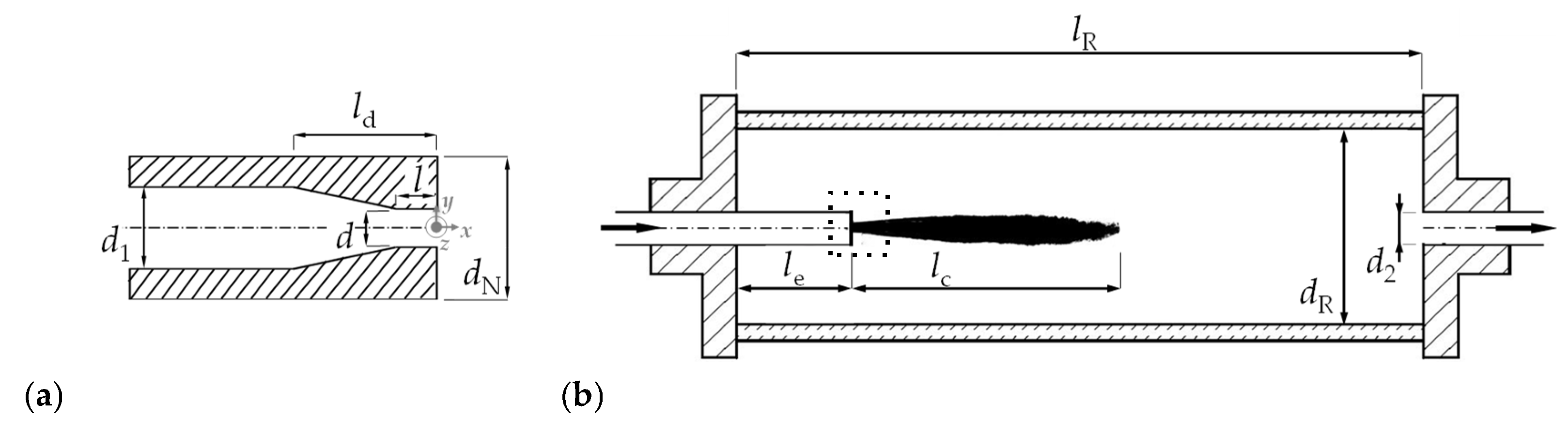
| Parameter | ||||||||
|---|---|---|---|---|---|---|---|---|
| numerical value | 3 mm | 12 mm | 5.5 mm | 2.5 | 9 mm | 25 mm | 150 mm | 30 mm |
2.2. Measurement of Process Variables
3. Process Characterization
3.1. Influencing Effects and Dimensionless Numbers
3.2. Materials and Methods for Process Evaluation
3.2.1. Investigation of Dye Degradation
3.2.2. Length of the Cavitating Jet and Sound Emission
3.2.3. Investigation of Reactivity
4. Degradation Process
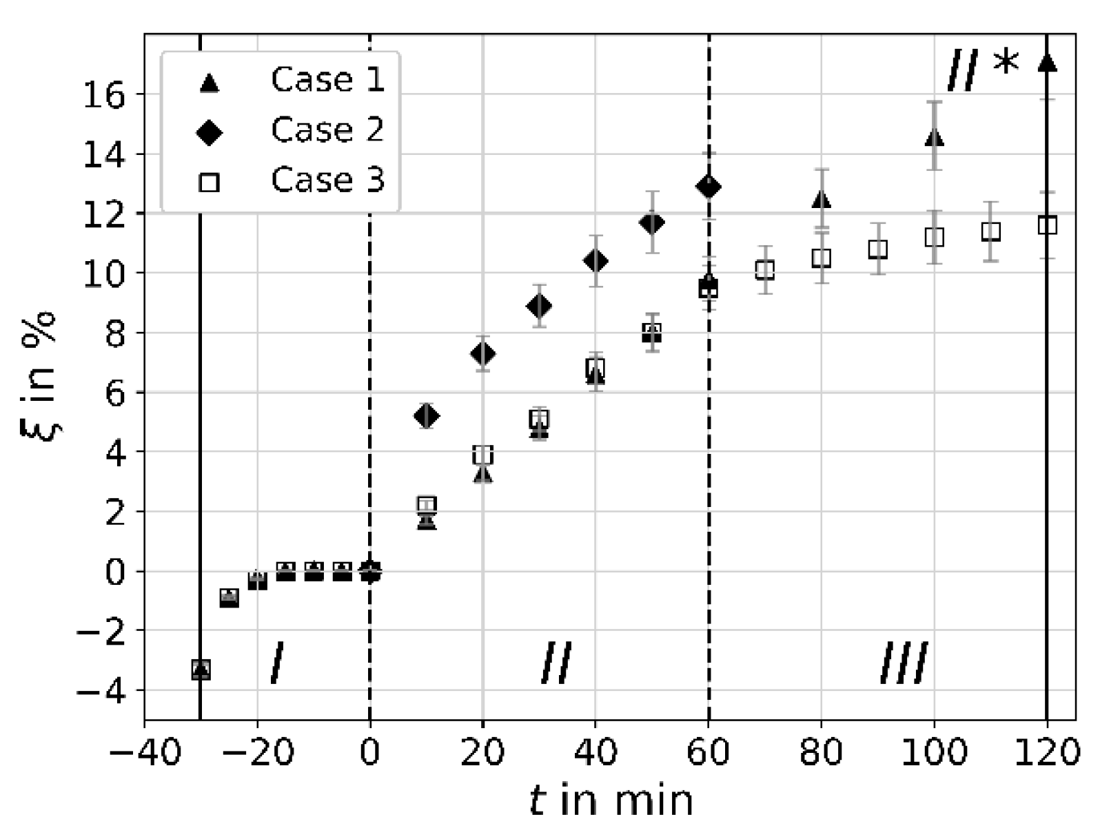
4.1. Procedure
4.2. Proof of Concept
4.3. Effect of Non-Cavitating Circulation
4.4. Efficiency and Degassing
5. Conditions and Reactivity of the Flow
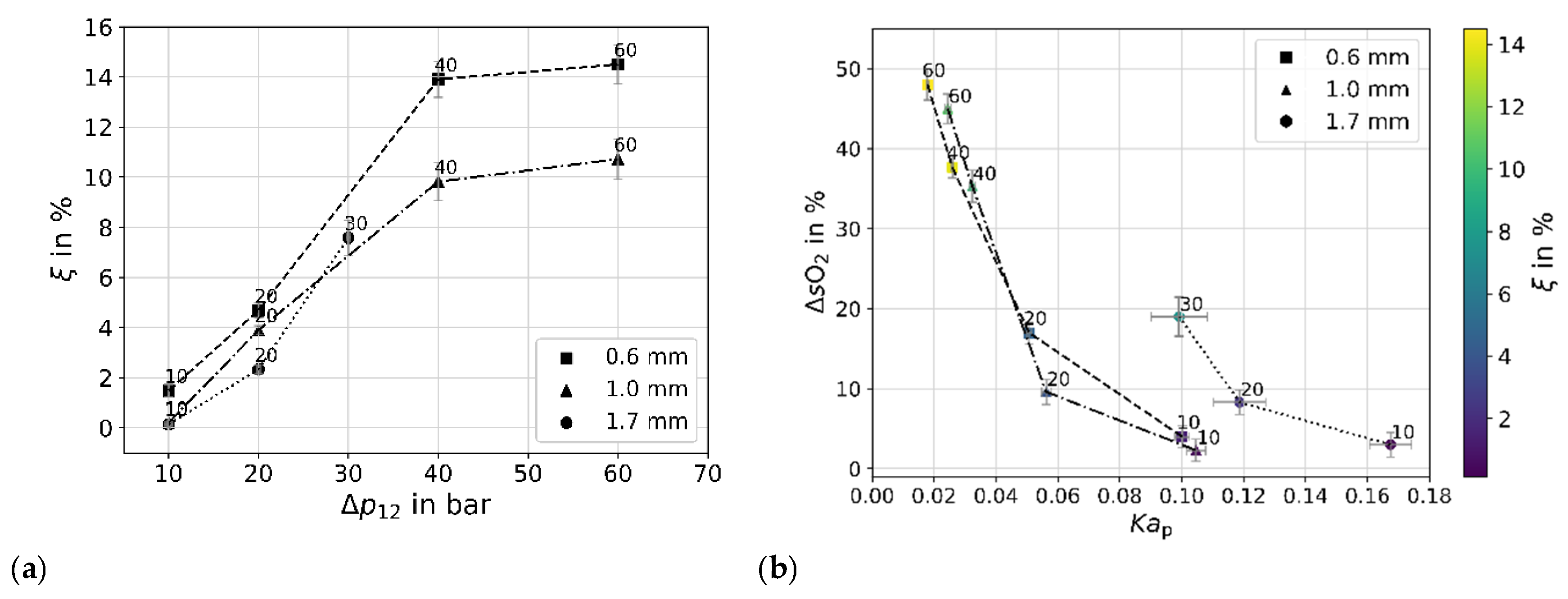
5.1. Flow Conditions
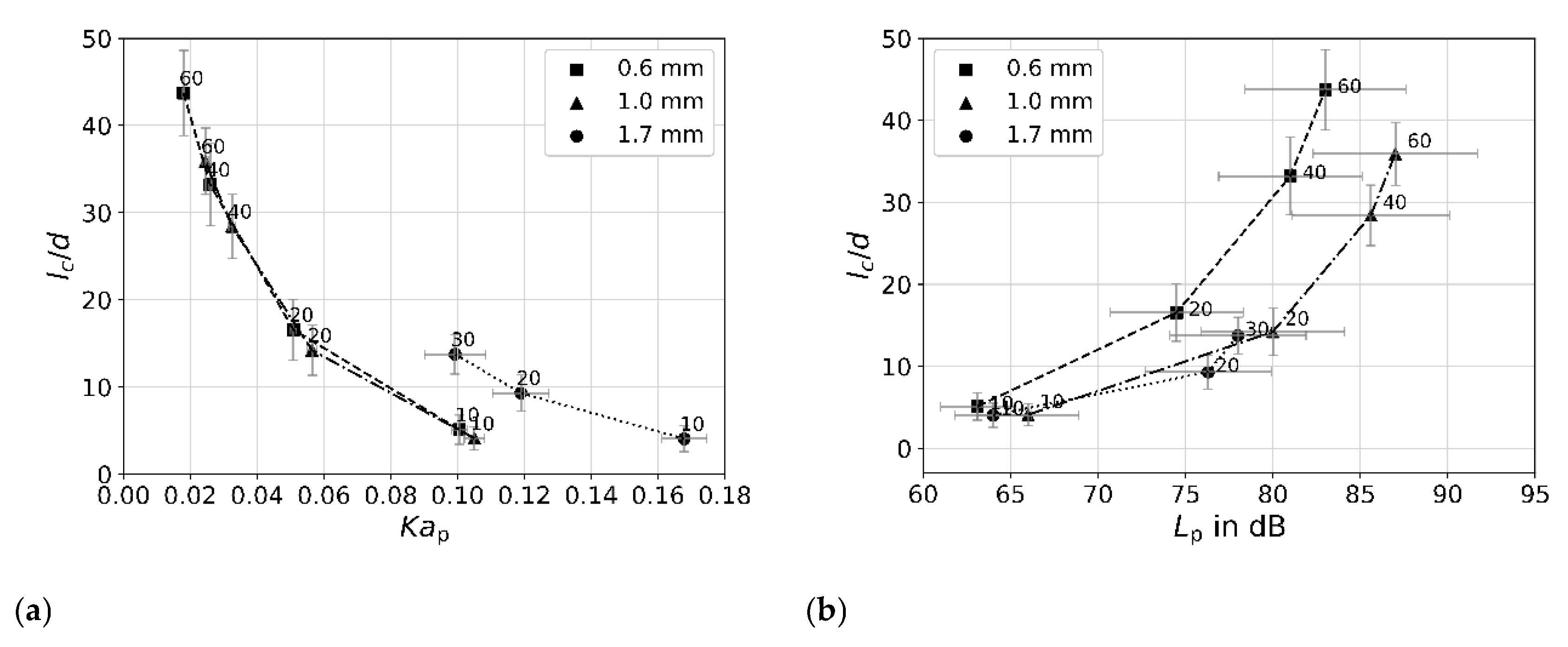
5.2. Cavitation Jet Length and Acoustic Sound Emission
5.3. Reactivity
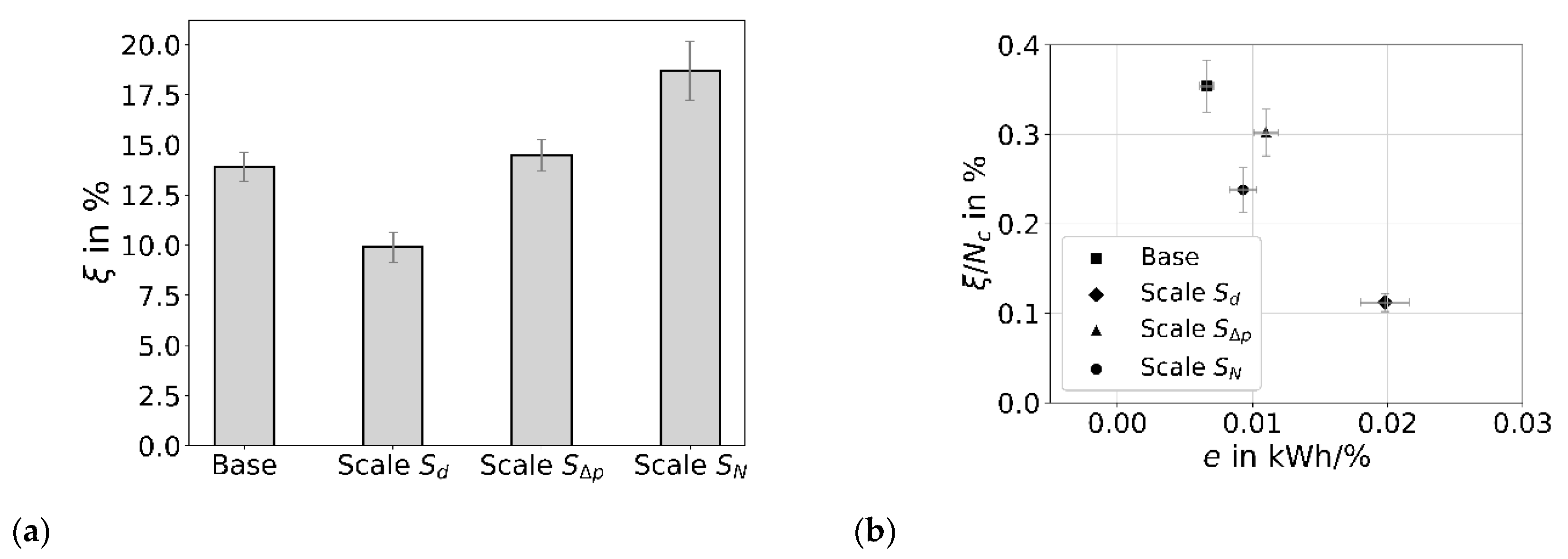
6. Aspects of Scalability
7. Conclusions
Author Contributions
Funding
Data Availability Statement
Conflicts of Interest
References
- Yaseen, D.A.; Scholz, M. Textile dye wastewater characteristics and constituents of synthetic effluents: A critical review. Int. J. Environ. Sci. Technol. 2019, 16, 1193–1226. [Google Scholar] [CrossRef]
- Tkaczyk, A.; Mitrowska, K.; Posyniak, A. Synthetic organic dyes as contaminants of the aquatic environment and their implications for ecosystems: A review. Sci. Total Environ. 2020, 717, 137222. [Google Scholar] [PubMed]
- Suslick, K.S.; McNamara, W.B.; Didenko, Y. Hot Spot Conditions During Multi-Bubble Cavitation. In Sonochemistry and Sonoluminescence; Crum, L.A., Mason, T.J., Reisse, J., Suslick, K.S., Eds.; Kluwer Publishers: Dordrecht, The Netherlands, 1999; pp. 191–204. [Google Scholar]
- Suslick, K.S.; Mdleleni, M.M.; Ries, J.T. Chemistry induced by hydrodynamic cavitation. J. Am. Chem. Soc. 1997, 119, 9303–9304. [Google Scholar] [CrossRef]
- Saharan, V.K.; Badve, M.P.; Pandit, A.B. Degradation of Reactive Red 120 dye using hydrodynamic cavitation. Chem. Eng. J. 2011, 178, 100–107. [Google Scholar]
- Zupanc, M.; Kosjek, T. Petkovšek, M.; Dular, M.; Kompare, B.; Širok, B. Stražar, M. Heath, E. Shear-induced hydrodynamic cavitation as a tool for pharmaceutical micropollutants removal from urban wastewater. Ultrason. Sonochem. 2014, 21, 1213–1221. [Google Scholar]
- Askarniya, Z.; Sadeghi, M.-T.; Baradaran, S. Decolorization of Congo red via hydrodynamic cavitation in combination with Fenton’s reagent. Chem. Eng. Process. Process. Intensif. 2020, 150, 107874. [Google Scholar]
- Bandala, E.R.; Rodriguez-Narvaez, O.M. On the Nature of Hydrodynamic Cavitation Process and Its Application for the Removal of Water Pollutants. Air Soil Water Res. 2019, 12, 1178622119880488. [Google Scholar] [CrossRef]
- Abbas-Shiroodi, Z.; Sadeghi, M.-T.; Baradaran, S. Design and optimization of a cavitating device for Congo red decolorization: Experimental investigation and CFD simulation. Ultrason. Sonochem. 2021, 71, 105386. [Google Scholar]
- Kumar, M.S.; Sonawane, S.; Pandit, A.B. Degradation of methylene blue dye in aqueous solution using hydrodynamic cavitation based hybrid advanced oxidation processes. Chem. Eng. Process. Process. Intensif 2017, 122, 288–295. [Google Scholar] [CrossRef]
- Cai, M.; Su, J.; Zhu, Y.; Wei, X.; Jin, M.; Zhang, H.; Dong, C.; Wie, Z. Decolorization of azo dyes Orange G using hydrodynamic cavitation coupled with heterogeneous Fenton process. Ultrason. Sonochem. 2016, 28, 302–310. [Google Scholar]
- Rajoriya, S.; Bargole, S.; Saharan, V.K. Degradation of reactive blue 13 using hydrodynamic cavitation: Effect of geometrical parameters and different oxidizing additives. Ultrason. Sonochem. 2017, 37, 192–202. [Google Scholar] [PubMed]
- Baradaran, S.; Sadeghi, M.T. Coomassie Brilliant Blue (CBB) degradation using hydrodynamic cavitation, hydrogen peroxide and activated persulfate (HC-H2O2-KPS) combined process. Chem. Eng. Process. -Process Intensif. 2019, 145, 107674. [Google Scholar]
- Nöpel, J.-A.; Fröhlich, J.; Rüdiger, F. Experimental investigation of cavitation in a jet regarding process optimization. In the Proceedings of 11th International Symposium on Cavitation, Daejon, Republic of Korea, 10–13 May 2021. [Google Scholar]
- Zupanc, M.; Pandur, Ž.; Perdih, T.S.; Stopar, D.; Petkovšek, M.; Dular, M. Effects of cavitation on different microorganisms: The current understanding of the mechanisms taking place behind the phenomenon. A review and proposals for further research. Ultrason. Sonochem. 2019, 57, 147–165. [Google Scholar] [CrossRef] [PubMed]
- Siddiqui, S.I.; Allehyani, E.S.; Al-Harbi, S.A.; Hasan, Z.; Abomuti, M.A.; Rajor, H.K.; Oh, S. Investigation of Congo Red Toxicity towards Different Living Organisms: A Review. Processes 2023, 11, 807. [Google Scholar] [CrossRef]
- Merdoud, R.; Aoudjit, F.; Mouni, L.; Ranade, V.V. Degradation of methyl orange using hydrodynamic Cavitation, H2O2, and photo-catalysis with TiO2-Coated glass Fibers: Key operating parameters and synergistic effects. Ultrason. Sonochemistry 2024, 103, 106772. [Google Scholar] [CrossRef]
- Nöpel, J.-A.; Fröhlich, J.; Rüdiger, F. Impact of outgassing on dye degradation in jet cavitation. Chem. Eng. Sci. 2025, 302 Pt B, 120937. [Google Scholar] [CrossRef]
- Buckingham, E. On Physically Similar Systems; Illustrations of the Use of Dimensional Equations. Phys. Rev. 1914, 4, 345–376. [Google Scholar] [CrossRef]
- Šarc, A.; Stepišnik-Perdih, T.; Petkovšek, M.; Dular, M. The issue of cavitation number value in studies of water treatment by hydrodynamic cavitation. Ultrason. Sonochemistry 2017, 34, 51–59. [Google Scholar] [CrossRef]
- Nöpel, J.-A.; Ayela, F. Experimental evidences of radicals production by hydrodynamic cavitation: A short review. Comptes Rendus Chimie 2023, 26, 157–166. [Google Scholar] [CrossRef]
- Rood, K.M.; Buhimschi, C.S.; Dible, T.; Webster, S.; Zhao, G.; Samuels, P.; Buhimschi, I.A. Congo Red Dot Paper Test for Antenatal Triage and Rapid Identification of Preeclampsia. EClinMed. 2019, 8, 47–56. [Google Scholar] [CrossRef]
- El-Meanawy, A.; Mueller, C.; Iczkowski, K.A. Improving sensitivity of amyloid detection by Congo red stain by using polarizing microscope and avoiding pitfalls. Diagn Pathol. 2019, 14, 57. [Google Scholar] [CrossRef] [PubMed]
- Dawood, S.; Sen, T.K. Removal of anionic dye Congo red from aqueous solution by raw pine and acid-treated pine cone powder as adsorbent: Equilibrium, thermodynamic. Water Res. 2012, 46, 1933–1946. [Google Scholar] [CrossRef] [PubMed]
- Frid, P.; Anisimov, S.V.; Popovic, N. Congo red and protein aggregation in neurodegenerative diseases. Brain Res Rev. 2007, 53, 135–160. [Google Scholar] [PubMed]
- Mittal, A.; Mittal, J.; Malviya, A.; Gupta, V.K. Adsorptive removal of hazardous anionic dye “Congo red” from wastewater using waste materials and recovery by desorption. J. Colloid Interface Sci. 2009, 340, 16–26. [Google Scholar] [CrossRef]
- Al-Tohamy, R.; Ali, S.S.; Li, F.; Okasha, K.M.; Mahmoud, Y.A.-G.; Elsamahy, T.; Jiao, H.; Fu, Y.; Sun, J. A critical review on the treatment of dye-containing wastewater: Ecotoxicological and health concerns of textile dyes and possible remediation approaches for environmental safety. Ecotoxicol. Environ. Saf. 2022, 231, 113160. [Google Scholar]
- Nöpel, J.-A.; Zedler, Z.; Deggelmann, M.; Braeutigam, P.; Fröhlich, J.; Rüdiger, F. Experimental investigation of the bubble distribution and chemical reactions induced by hydrodynamic cavitation inside a reactor—A preliminary study. In the Proceedings of 5th International Conference on Experimental Fluid Mechanics ICEFM, Munich, Germany, 2–4 July 2018. [Google Scholar]
- DIN EN ISO 1683:2015-09; Acoustics—Preferred reference values for acoustical and vibratory levels (ISO 1683:2015). ISO: Geneva, Switzerland, 2015.
- Dorfmann, L.M.; Adams, G.E. Reactivity of the Hydroxyl Radical in Aqueous Solutions; National Bureau of Standards: Washington, DC, USA, 1973. [Google Scholar]
- Munter, R. Advanced oxidation processes: Current status and prospects. Proc. Estonian. Acad. Sci. Chem. 2001, 50, 59–80. [Google Scholar]
- Renaudin, V.; Gondrexon, N.; Boldo, P.; Pétrier, C.; Bernis, A.; Gonthier, Y. Method for determining the chemically active zones in a high-frequency ultrasonic reactor. Ultrason. Sonochem. 1994, 1, 81–85. [Google Scholar]
- Deggelmann, M.; Nöpel, J.-A.; Rüdiger, F.; Paustian, D.; Braeutigam, P. Hydrodynamic cavitation for micropollutant degradation in water—Correlation of bisphenol A degradation with fluid mechanical properties. Ultrason. Sonochem. 2022, 83, 105950. [Google Scholar]
- Thanekar, P.; Gogate, P.R.; Znak, Z.; Sukhatskiy, Y.; Mnykh, R. Degradation of benzene present in wastewater using hydrodynamic cavitation in combination with air. Ultrason. Sonochem. 2021, 70, 105296. [Google Scholar] [CrossRef]
- Yasui, K. Chemical reactions in a sonoluminescing bubble. J. Phys. Soc. Jpn. 1997, 66, 2911–2920. [Google Scholar]
- Soyama, H. Key factors and applications of cavitation peening. Int. J. Peening Sci. Technol. 2017, 1, 3–60. [Google Scholar]
- Nöpel, J.-A.; Frense, E.; Korb, S.; Dues, M.; Rüdiger, F. Velocity measurement of a free jet in water with shear layer cavitation. In the Proceedings of 27th Conference Experimental Fluid Mechanics, Erlangen, Germany, 3–5 September 2019. [Google Scholar]
- Nöpel, J.-A.; Krieger, M.; Frense, E.; Rüdiger, F. Characterization of air outgassing process in dye degradation experiments using hydrodynamic jet cavitation. In the Proceedings of 29th Conference Experimental Fluid Mechanics, Ilmenau, Germany, 5–7 September 2022. [Google Scholar]
- Brennen, C.E. Cavitation and Bubble Dynamics; Cambridge University Press: Cambridge, UK, 2013. [Google Scholar]
- McKinley, G.H.; Renardy, M. Wolfgang von Ohnesorge. Phys. Fluids 2011, 23, 127101. [Google Scholar] [CrossRef]


| i | 1 | 2 | 3 | 4 | 5 | 6 | 7 | 8 |
| Physical Meaning | ||
|---|---|---|
| Cavitation number based on diameter. Indicates tendency of the flow to cavitate. | ||
| Cavitation number without geometrical influence, ratio of pressure difference reactor to phase change divided by the pressure drop of the nozzle inlet and reactor. Indicates tendency of the flow to cavitate. | ||
| Reynolds number, ratio of inertial to viscous force. Indicates the flow regime. | ||
| Gas dissolution potential. Indicates the potential for degassing due to cavitation. | ||
| Weber number, ratio of inertial to surface tension forces. Indicates bubble deformation. | ||
| number. Indicates interface stability. | ||
| OX value, ratio of dissolved oxygen fraction at starting condition in water. A criterion for possible degassing. | ||
| RS value, ratio of reactor length to diameter. Indicates the local conditions in the reactor. A measure of recirculation and pressure gradient. |
| Configuration | GDP | |||||
|---|---|---|---|---|---|---|
| 0602 | 0.51 | 0.49 | 9400 | 0.010 | 1600 | 0.180 |
| 0620 | 0.06 | 0.05 | 28,700 | 0.048 | 15,100 | 0.180 |
| 0640 | 0.03 | 0.03 | 40,800 | 0.067 | 30,600 | 0.180 |
| 0660 | 0.02 | 0.02 | 49,900 | 0.102 | 45,600 | 0.180 |
| 1002 | 0.46 | 0.49 | 16,500 | 0.020 | 3000 | 0.108 |
| 1020 | 0.09 | 0.06 | 39,500 | 0.142 | 17,100 | 0.108 |
| 1040 | 0.05 | 0.03 | 54,800 | 0.254 | 33,000 | 0.108 |
| 1060 | 0.04 | 0.02 | 66,600 | 0.341 | 48,800 | 0.108 |
| 1702 | 0.90 | 0.56 | 21,500 | 0.142 | 3000 | 0.064 |
| 1710 | 0.31 | 0.17 | 44,600 | 0.423 | 12,900 | 0.064 |
| 1720 | 0.22 | 0.12 | 62,300 | 0.593 | 25,100 | 0.064 |
| 1730 | 0.19 | 0.10 | 76,000 | 0.675 | 37,400 | 0.064 |
| Investigation | Dye degradation | Cavitating jet length and acoustic sound emission | Flow reactivity by hydroxyl radicals |
| Material | DI water, Congo red | DI water | DI water, luminol, NaHCO3 |
| Objective | Degradation level and rate | Cavitation length and acoustic sound emission | Detection of reactive areas |
| Method | Absorbance measurement using UV-Vis spectroscopy | Image acquisition and processing with laser light sheet illumination; sound level measurement | Long exposure image acquisition of chemiluminescence |
| Device | Effect to Prevent | Countermeasure |
|---|---|---|
| pipe system, tank, pump | adhesion to surface | stainless steel |
| large tank | sedimentation | stirrer |
| pump | cavitation | installation of piston pumps |
| Configuration | 0640 | 1040 | 1730 |
|---|---|---|---|
| in % | 23.5 | 17.0 | 13.3 |
| in 1/s | 3.7 × 10⁻⁵ | 2.6 × 10⁻⁵ | 2.0 × 10⁻⁵ |
| in MJ | 0.6 | 1.4 | 2.5 |
| 2 | 4.5 | 7.9 |
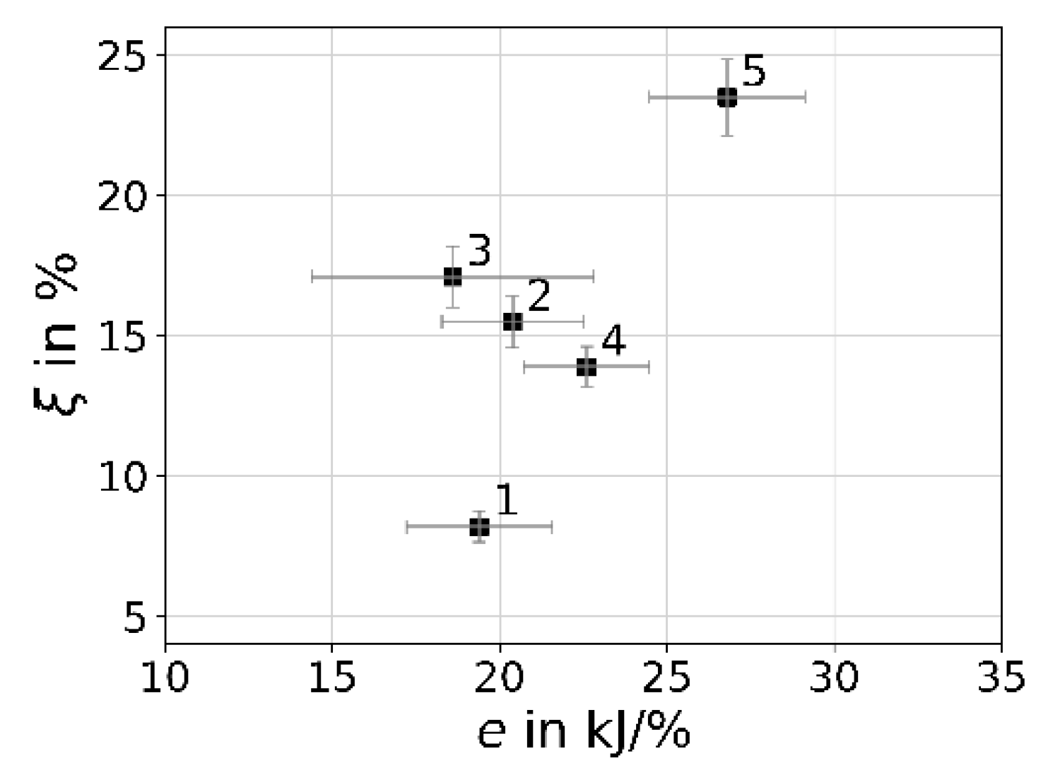
| Case | Procedure Phase | Degradation ξ per Phase in % | Energy E in kJ | Specific Energy e in kJ/% |
|---|---|---|---|---|
| 1 | CAV 30 min; CIR 30 min | 6.8 + 1.5 = 8.2 | 159 | 19.4 |
| 2 | CAV 60 min; CIR 30 min | 13.9 + 1.6 = 15.5 | 316 | 20.4 |
| 3 | 2 times Case 1 | 6.8 + 1.5 + 7.1 + 1.7 = 17.1 | 318 | 18.6 |
| 4 | CAV 60 min | 13.9 | 314 | 22.6 |
| 5 | CAV 120 min | 23.5 | 629 | 26.8 |
| Parameters and Similarity Numbers | 0640 | 1040 | 1730 |
|---|---|---|---|
| = 2 h) | 23.5 | 17.0 | 13.3 |
| in bar | 40 | 40 | 30 |
| in L/min | 1.3 | 2.9 | 6.9 |
| in bar | 1.0 | 1.3 | 3.0 |
| in % | 37 | 35 | 19 |
| 0.03 | 0.05 | 0.19 | |
| 0.03 | 0.03 | 0.10 | |
| 39,700 | 53,300 | 73,900 | |
| 30,600 | 33,000 | 37,400 | |
| 0.180 | 0.108 | 0.064 | |
| 0.07 | 0.25 | 0.67 |
| Case | Ratio to 0640 | Case | in L/min | in 1/s | /VT in kWh/m3 | in bar | in % | ||
|---|---|---|---|---|---|---|---|---|---|
| Base | - | 0640 | 1.3 | 4.2 × 10⁻⁵ | 1.11 | 1.07 | 37 | 0.025 | 39,700 |
| = 1.67 | 1040 | 2.9 | 2.9 × 10⁻⁵ | 1.11 | 1.31 | 35 | 0.032 | 53,300 | |
| = 1.5 | 0660 | 1.6 | 4.4 × 10⁻⁵ | 1.67 | 1.11 | 48 | 0.018 | 48,500 | |
| = 2 | 2 × 0640 | 2.6 | 5.8 × 10⁻⁵ | 1.11 | 1.09 | 31 | 0.026 | 39,700 |
Disclaimer/Publisher’s Note: The statements, opinions and data contained in all publications are solely those of the individual author(s) and contributor(s) and not of MDPI and/or the editor(s). MDPI and/or the editor(s) disclaim responsibility for any injury to people or property resulting from any ideas, methods, instructions or products referred to in the content. |
© 2025 by the authors. Licensee MDPI, Basel, Switzerland. This article is an open access article distributed under the terms and conditions of the Creative Commons Attribution (CC BY) license (https://creativecommons.org/licenses/by/4.0/).
Share and Cite
Nöpel, J.-A.; Fröhlich, J.; Rüdiger, F. Experimental Study of Dye Degradation in a Single-Jet Cavitation System. Processes 2025, 13, 1088. https://doi.org/10.3390/pr13041088
Nöpel J-A, Fröhlich J, Rüdiger F. Experimental Study of Dye Degradation in a Single-Jet Cavitation System. Processes. 2025; 13(4):1088. https://doi.org/10.3390/pr13041088
Chicago/Turabian StyleNöpel, Julius-Alexander, Jochen Fröhlich, and Frank Rüdiger. 2025. "Experimental Study of Dye Degradation in a Single-Jet Cavitation System" Processes 13, no. 4: 1088. https://doi.org/10.3390/pr13041088
APA StyleNöpel, J.-A., Fröhlich, J., & Rüdiger, F. (2025). Experimental Study of Dye Degradation in a Single-Jet Cavitation System. Processes, 13(4), 1088. https://doi.org/10.3390/pr13041088