Integrated Data-Driven Framework for Forecasting Tight Gas Production Based on Machine Learning Algorithms, Feature Selection and Fracturing Optimization

Abstract

A precise assessment of tight gas operational efficiency is critical for investment decisions in unconventional reservoir development. However, quantifying production efficiency remains challenging due to the complex relationships between geological and operational factors. This study proposes a novel data-driven framework for predicting tight gas productivity, effectively integrating computing algorithms, machine learning algorithms, feature selection, production prediction and fracturing parameter optimization. A dataset of 3146 horizontal wells from the Montney tight gas field was used to train six machine learning models, aiming to identify the most significant factors. Results indicate that fluid-injection volumes, burial depth, number of stages, Young’s modulus, formation pressure, saturation, sandstone thickness and total organic carbon are the key variables for tight gas production. The Random Forest-based model achieved the highest accuracy of 88.6%. Case studies for the test demonstrate well that gas production could be nearly doubled by increasing fracturing fluid injection by 97.5%. This work provides evidence-based recommendations to refine development strategies and maximize reservoir performance.

1. Introduction

In recent years, global demand for clean energy sources such as unconventional natural gas has surged, due to a decline in traditional fossil fuel reserves and growing concerns over the greenhouse effect and air pollution [1]. Tight gas has become a focus of global oil and gas exploration, with the estimated worldwide resources to be about 210 × 10¹² m³, accounting for 75% of unconventional gas reserves [2]. However, compared to conventional reservoirs, tight gas reservoirs pose significant exploitation challenges [3]. Their pore types are dominated by secondary porosity, and gas seepage channels rely heavily on fracture networks [4,5]. These reservoirs exhibit extreme heterogeneity in reservoir properties [6,7,8], compounded by difficulties in accurately measuring geological and engineering parameters in real time [9,10,11]. Additionally, tight gas reservoir blocks are usually typified by massive, heterogeneous field datasets characterized by poor data regularity and complex processing requirements, which impede rapid, accurate production prediction and delay the establishment of predictive models to guide reservoir development [12,13]. Consequently, a swift and reliable method is required to predict tight gas production to address the accelerating field development [14,15,16].

With the arrival of the big data era and the development of oil and gas field automation, machine learning (ML) methods provide an effective way for the digitalization of oil and gas field development [17,18,19]. By combining the well production-prediction research with the digital oil and gas field workflows, a new ML method has been developed to quantify production efficiency and unravel complex relationships between geological and operational factors [20,21,22]. It can quantify the contribution of individual factors to outcomes, and enable reliable predictions under different controlling factors.

This paper proposes a novel data-driven approach for predicting tight gas production, effectively integrating machine learning algorithm comparison, feature selection, production prediction and fracturing parameter optimization.

The process begins with the database collection of geological and engineering parameters from the Montney tight gas field, which includes 3146 horizontal wells. Next, six machine learning methods, namely Extreme Gradient Boosting Tree (XGBoost), Random Forest (RF), Gradient Boosting Decision Tree (GBDT), Artificial Neural Networks (ANN), Light Gradient Boosting Tree (LightGBM) and Extreme Randomized Tree (ET), are trained. These trained models serve to forecast production performance and quantify the contribution of geological and engineering factors to production outcomes. Operational plans are then optimized to maximize productivity by adjusting the fracturing fluid injection and proppant mass through the optimal calculating algorithm. This methodology establishes a comprehensive closed-loop process that covers evaluation, forecasting and optimization. This work presents the following novelties and contributions:

• This framework introduces machine learning-based predictions for tight gas development and provides new insights into the key features that influence tight gas production. By integrating machine learning algorithms, feature selection, production prediction and fracturing parameter optimization, it can effectively develop tight gas resources.
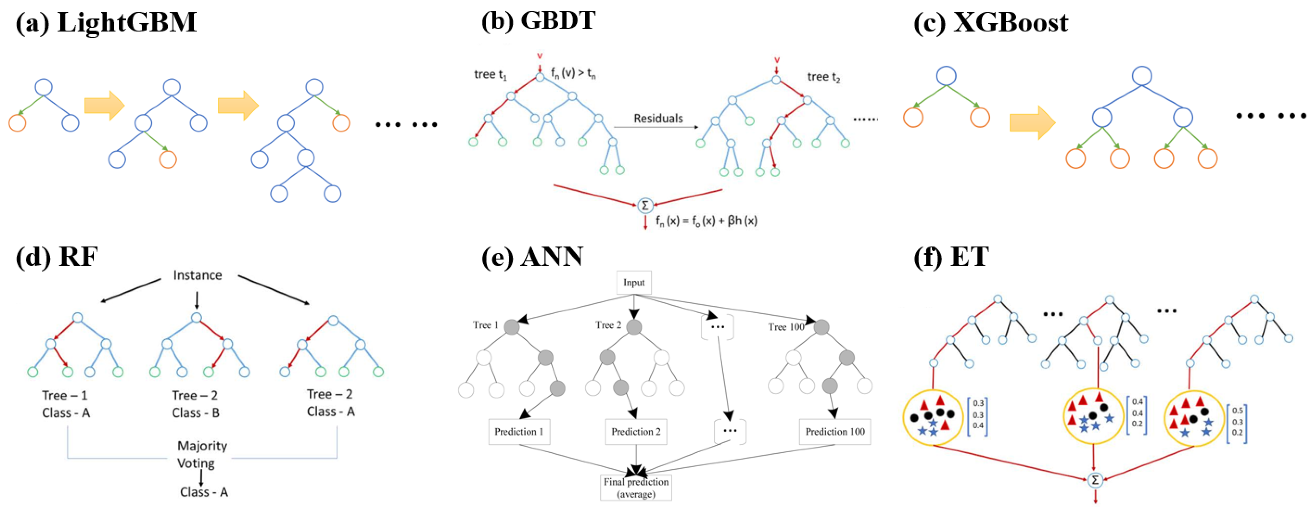
• A distinctive aspect of the study is the in-depth comparison of feature-selection techniques. The framework combines six methods (i.e., XGBoost, RF, GBDT, ANN, LightGBM and ET) with six machine learning models to provide a comprehensive assessment and comparative understanding. The most effective machine learning algorithm, along with the most significant factors, is identified.
• The most important aspect of this research is the optimization of fracturing parameters based on the best-performing machine learning model. Operational plans are fine-tuned to maximize productivity by adjusting the fracturing fluid injection and proppant mass using the optimal algorithm.

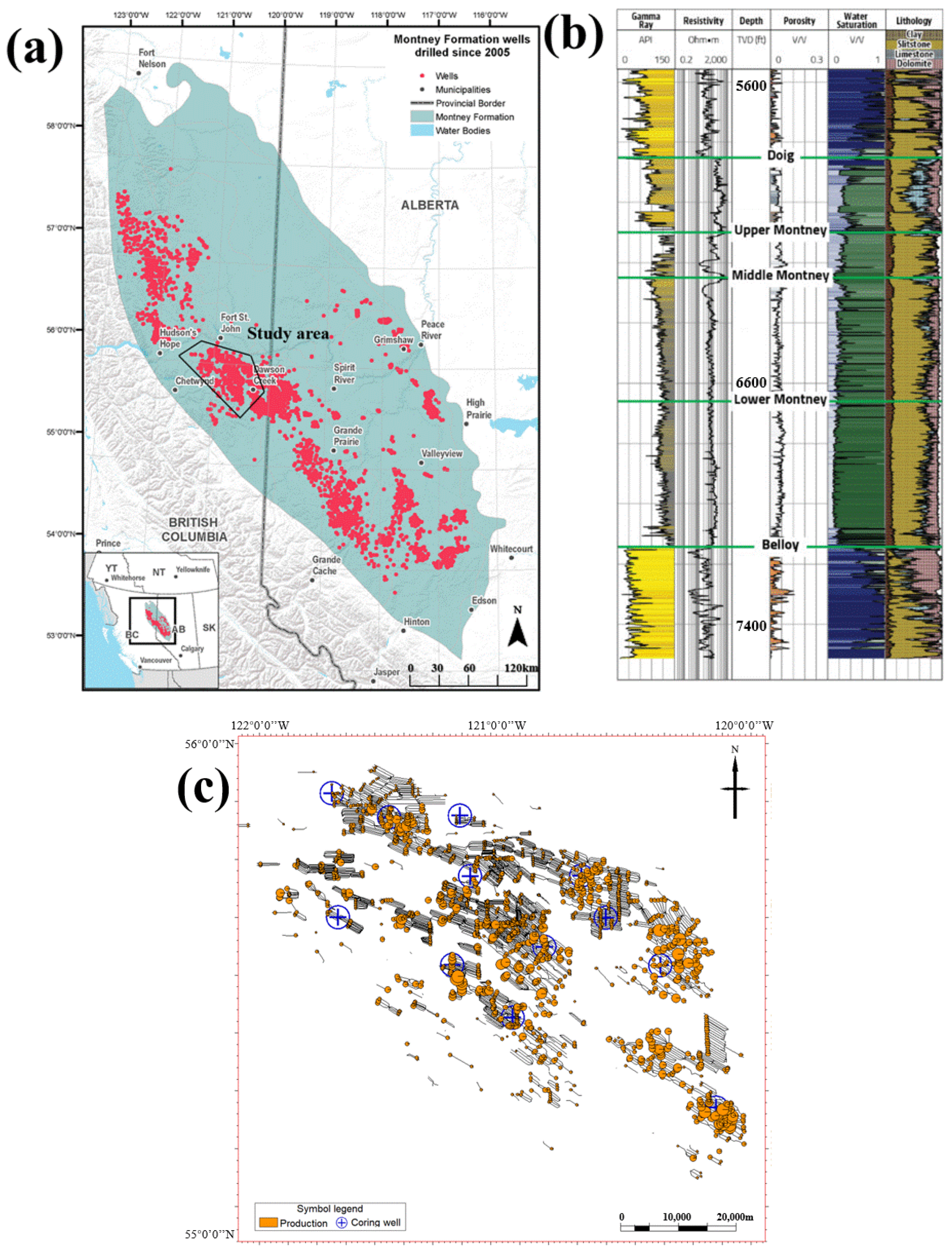
2. Field Background

The study area is located in the Montney Formation of the Triassic of the Western Canada Sedimentary Basin, which is mainly distributed in the northwestern part of the basin, gradually thinning eastward until it is stripped out (Figure 1a) [23,24,25]. The Montney Formation is a wedge-shaped, unconsolidated deposit formed along stable Carboniferous and Permian cratonic margins. As a semi-deep-sea deposition, it exceeds 1200 m in thickness and features sand bodies oriented northeast–southwest [26]. The lithology of the Montney Formation transitions from siltstone to mudstone, with interbedded sandstone and siltstone. The Montney section is mainly composed of organic-rich, radioactive shale and dense siltstone, which are generally recognized as high-quality reservoir intervals.

The Montney gas field has burial depths of 1700–4000 m, a thickness of 300 m, a gas porosity of 1.0–6.0% and reserves of 80–700 trillion cubic feet (Figure 1b) [27,28]. Characterized by secondary pores and fracture-dominated seepage channels, the tight sandstone reservoir features high irreducible water saturation, elevated capillary pressure, dense rock matrices and complex pore–throat networks, resulting in poor fluid mobility and pronounced heterogeneity [29]. These attributes render conventional production-forecasting methods inadequate for tight gas well analysis.

This section summarizes the geological characteristics and production dynamics of the tight gas field in the Montney field, establishing a foundation for the subsequent research work. Data collected from the GeoScout database (https://www.geologic.com/products/geoscout/, accessed on 1 February 2025) include drilling, completion, fracturing and production records for 3146 wells, alongside core analysis data from 12 cored intervals (Figure 1c).

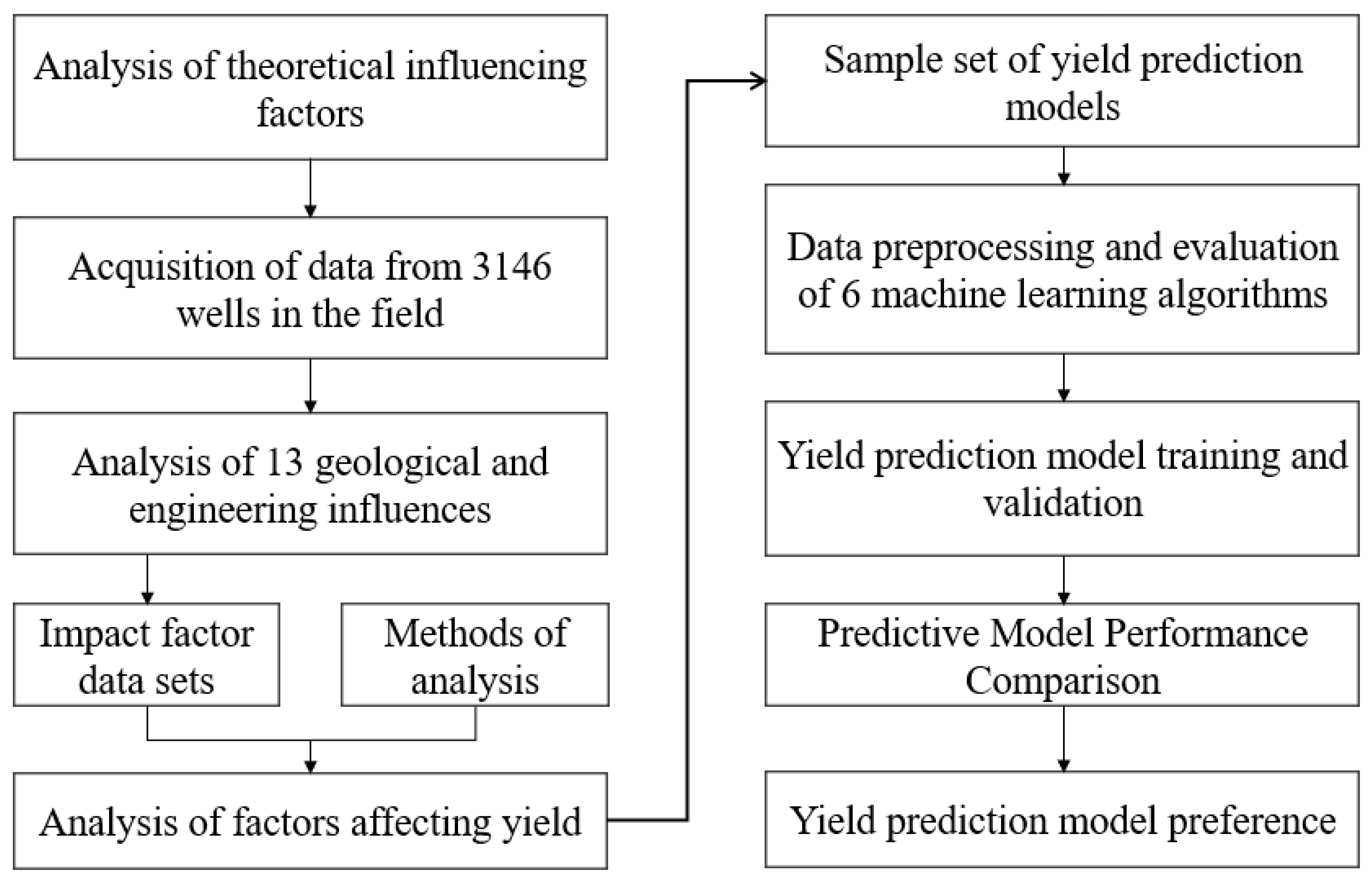
3. Methodology

This research aims at the tight sandstone oil and gas reservoirs in the Montney area. Based on previous research, it combines advanced theories and technologies like big data and artificial intelligence. The objective is to intelligently predict the production of tight gas wells in the researched area and construct a production capacity-prediction model for tight gas fracturing horizontal wells using a machine learning method (Figure 2). The data from the oil and gas field mainly includes geological and engineering data.

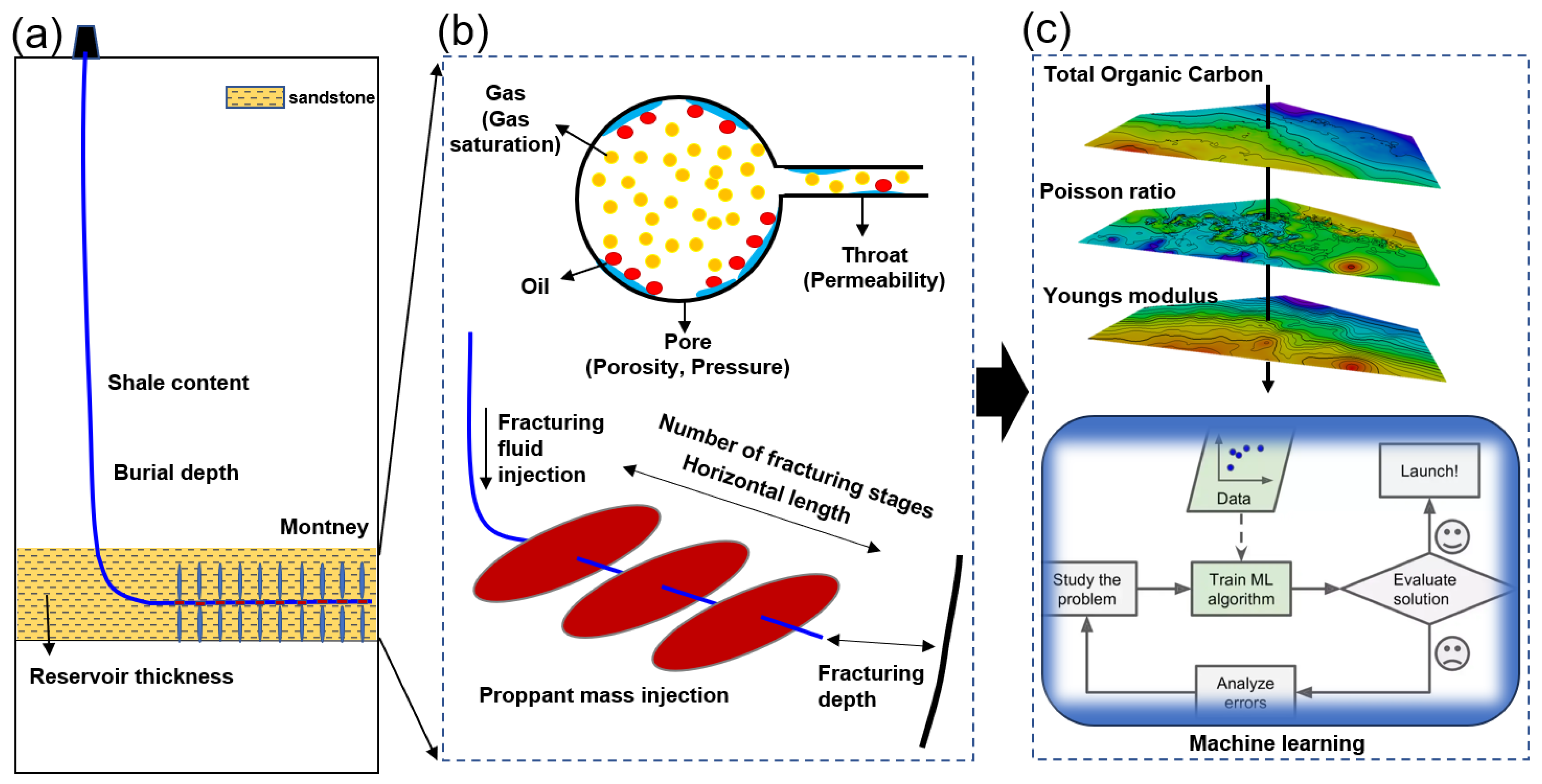
3.1. Parameter Characterization and Selection

Before constructing the production-prediction model for tight gas wells, it is essential to evaluate the feature dispersion of the dataset [30]. Feature selection requires systematic analysis of the relationship strength between parameters and production capacity, aiming to eliminate irrelevant variables while preserving geologically and statistically significant features. This process reduces the model complexity without sacrificing critical predictive factors [31]. The Pearson correlation coefficient is employed as a quantitative criterion to prioritize features strongly correlated with target variables and to exclude parameters exhibiting excessive mutual correlations, including multicollinearity.

3.1.1. Parameter Characterization

When constructing the production-prediction model, in order to incorporate the data sources that control the production rate, it is imperative to analyze the factors affecting the production rate of the production wells in the Montney work area. Through a comprehensive analysis of the correlation between various geological and engineering factors and the production rate, the geological factors are identified as reservoir physical parameters, specifically sandstone porosity and gas saturation; preservation conditions, as burial depth, pressure and thickness; and shale content, Poisson ratio, total organic carbon and young’s modulus (Figure 3a) [32,33]. On the engineering side, the parameters include cumulative fluid injection, cumulative proppant injection, the number of stages and the horizontal length of the wells (Figure 3b) [34].

By ranking the importance of these features, the key factors controlling production were selected as the input features for machine learning, laying a solid foundation for the subsequent production-prediction modeling [35]. Previous studies have clearly demonstrated that geological and engineering factors affect the production of tight gas following the fracturing process [36].

Table 1. Factors influencing tight gas production and data sources.

Typology	Influencing Factors	Data Sources	Representative Wells
Geological factors	Preservation conditions (burial depth, pressure and thickness)	Well-logging, well-completion and monitoring data	15-16-78-18
	Sandstone porosity and gas saturation Shale content, total organic carbon Poisson ratio, Young’s modulus	Core analysis	6-26-78-18
Engineering factors	Cumulative fluid injection, cumulative proppant injection	Fracturing construction information	6-10-79-15
	Number of stages, horizontal length	Fracturing construction information	15-2-80-16

systematically lists the factors that impact tight gas production, along with the corresponding data sources for each factor. These parameters will serve as input parameters in the machine learning-based computing models (Figure 3c).

(1)

Geological factors

In this paper, we primarily consider nine geological factors that affect oil production in sandstone reservoirs, which are formation pressure, sandstone thickness, burial depth, porosity, saturation, mud content, total organic carbon content, Poisson’s ratio and Young’s modulus. These geological factors were obtained through actual core measurements and well-log interpretation from the Montney sandstone field and relevant statistics were compiled.

The preservation conditions, serving as the external factors affecting the formation of tight gas, mainly include the regional tectonic background and the evolution of geological processes [37]. Previous literature predominantly focuses on the burial depth, pressure and sandstone thickness of tight gas reservoirs. The burial depth has an important impact on the economic value and benefits of tight gas reservoirs. Meanwhile, pressure significantly affects numerous characteristics of these reservoirs [38]. For example, temperature has an important effect on the adsorbed gas content with reservoirs [39]. The adsorbed gas content decreases as the temperature rises because the gas molecules move and the adsorbed gas content is lower. Similarly, higher pressure enhances gas content until reaching the desired point more quickly. In a saturation threshold, beyond which the adsorption rate diminishes, a similar vein grows with increasing pressure; however, this decreases beyond a point.

Porosity, permeability and saturation are three dominant characteristics of sandstone reservoirs. The micropores in sandstones contain a good quantity of crude oil and free gas; thus, the magnitude of the porosity generally dictates the free gas content [40,41]. The mineralogical composition of sandstones not only affects the petrophysical properties of shales but also influences the degree of fracture development, which in turn has an impact on the distribution of tight gas “deserts”.

(2)

Engineering factors

The fracturing engineering on tight gas horizontal wells directly affects both the production rate and its prediction. In this study, the predominant focus is on the engineering factors that impact gas production in sandstone reservoirs, including the length of the horizontal section, the number of fracturing sections, the volume of fracturing fluid injection and the volume of proppant injection [42,43]. The engineering factors of the Montney tight gas field are obtained from the actual well drilling data and the completed fracturing parameters [44].

Notably, as the fracturing fluid injection volume and the number of fracturing stages increase, more fractures can be produced within sandstone reservoirs. Meanwhile, an increase in the volume of proppant injection and the length of the horizontal section is typically associated with a larger reservoir volume, promoting production, thereby contributing to an increase in tight gas production. However, it is essential to optimize the design of each fracturing parameter by considering both geological factors and engineering factors rather than simply maximizing them.

3.1.2. Parameter Correlation Analysis

The gas production of sandstone reservoirs is affected by multiple factors, mainly geologic factors (e.g., reservoir quality) and engineering factors (e.g., permeability and stimulation efficiency). In this paper, the Pearson correlation coefficient is initially applied to describe the relationships between geologic factors, engineering factors and production.

(1)

Correlation analysis expressions

The Pearson correlation coefficient, also known as the Pearson product–difference correlation coefficient, is commonly used to determine the correlation between two sets of continuous data that follow a bivariate normal distribution [45,46]. The Pearson correlation coefficient is symbolized as $r$, with its values ranging from −1 to 1. It is given by the following formula:

$$r={\displaystyle \frac{\sum _{i=1}^n\left(X_i-\overline{X}\right)\left(Y_i-\overline{Y}\right)}{\sqrt{\sum _{i=1}^n{\left(X_i-\overline{X}\right)}^2}\sqrt{\sum _{i=1}^n{\left(Y_i-\overline{Y}\right)}^2}}}$$

(1)

where $r$ is the correlation coefficient, $n$ is the sample size, $X$ and $Y$ are random variables and $\overline{X}$ and $\overline{Y}$ are their respective means. The denominator is the product of the standard deviations of $X$ and $Y$, while the numerator is the covariance. The covariance is used to characterize the correlation between two random variables $X$ and $Y$. The variance is a special form of the covariance and when the two variables are identical, the covariance is equivalent to the variance.

(2)

Classification of the degree of correlation

The Pearson correlation coefficient quantitatively describes the linear correlation between variables. A Pearson correlation coefficient $r>0$ indicates a positive correlation between the two variables, $r<0$ indicates a negative correlation and $r=0$ indicates the absence of a linear correlation. Moreover, the larger the absolute value of $r$, the more significant the influence of the factor on gas production [47] (

Table 2. Classification of degree of relevance [47].

Pearson Correlation Coefficient	Level of Relevance
0.00 <$\left|r\right|$< 0.20	Extremely weak correlation
0.21 <$\left|r\right|$< 0.40	Weak correlation
0.41 < $\left|r\right|$< 0.60	Moderately relevant
0.61 <$\left|r\right|$< 0.80	Strong correlation
0.81 <$\left|r\right|$< 1.00	Extremely Relevant

).

The Pearson correlation coefficient is used to analyze the geological and engineering parameters of tight gas, along with the production rate. This analysis can reveal the correlation between different geological and engineering parameters, as well as the correlation between each parameter and the production rate, thereby identifying the crucial parameters affecting the production rate of tight gas as the feature parameters in machine learning.

3.2. Machine Learning Methods

This work applies and compares six effective machine learning methods, namely Extreme Gradient Boosting Tree (XGBoost), Random Forest (RF), Gradient Boosting Decision Tree (GBDT), Artificial Neural Networks (ANN), Light Gradient Boosting Tree (LightGBM) and Extreme Randomized Tree (ET) [48,49] (Figure 4). The above-mentioned impacting parameters are adopted as the input variables and the output is natural gas production amounts over 6 months, 12 months and 18 months. The dataset is randomly divided into a training set and a test set. Thus, different computational models are assessed. The optimal prediction model is expected to exhibit the best performance in predicting natural gas production, possess the highest coefficient of determination and incur the smallest computational error [50,51,52].

3.2.1. Data Preprocessing

(1)

Dataset division

Considering the specificity of the oil and gas industry and the requirements for engineering inspection, the dataset is divided into two components with a ratio of 8:2 (training set:test set = 8:2). The training set is for model training and parameterization, establishing the relationship among geological parameters, fracturing construction parameters and the gas well production function [53]. The data within the test set are not involved in the model training process and its function is to evaluate the generalization ability of the model after the model has been built (the ability of the model to adapt to the unknown data). The entire process is calculated only once, effectively eliminating the interference of the human factor. And the prediction results of the test set can be used to verify the authenticity and applicability of the machine learning model [54,55].

(2)

Data normalization

Data normalization is a commonly used data preprocessing technique. Oil and gas data, geological parameters, fracturing parameters and gas well production values have distinct scales and exhibit significant differences in their value intervals. This leads to a lower convergence rate or even prevents convergence when solving the machine learning model. The original data are processed using the data normalization method, aiming to eliminate the influence of the scale differences among various factors. Data normalization not only transforms the data of different variables into the same range but also ensures that the sample values of each parameter fall within the interval of 0 and 1. For a specific feature $x$ in the sample set, the normalization formula is as follows:

$$x^{\text{'}}=\left(x-X_{min}\right)/\left(X_{max}-X_{min}\right)$$

(2)

where $x\text{'}$ is the normalized data, $x$ is the specific value in the data, X_min is the minimum value in the data and X_max is the maximum value in the data.

In this work, all machine learning models are trained and predicted with normalized data. Subsequently, all predicted data are reduced to the magnitude of the original data through inverse normalization.

3.2.2. Machine Learning Algorithms

(1)

Extreme Gradient Boosting Tree (XGBoost)

XGBoost consists of multiple regression trees, specifically CART decision trees. Each decision tree predicts the residual, which is calculated as the difference between the true value and the sum of the predicted values of all preceding decision trees. The predicted values of all the decision trees are then aggregated to obtain the final result [19].

XGBoost is widely used in classification, regression and sorting problems. The regression trees generate continuous regression values and the predicted values of multiple decision trees are summed up for the final outcome. For classification problems, which are divided into binary classification and multi-classification, XGBoost is well suited. In binary classification, the sigmoid function is employed by XGBoost to map the cumulative value within the range of 0~1, where the value represents the probability of the binary classification result. In the multi-class classification, the softmax function is used to map the multi-class prediction value between 0 and 1, representing the probability that a sample belongs to a specific category. The sorting problem will not be discussed.

(2)

Random Forest (RF)

Random Forest is an algorithm generated under the concept of ensemble learning. The core idea of ensemble learning is to provide a solution to the performance issues that a single model may encounter in certain aspects. It involves integrating a certain number of models to complement each other, thereby circumventing the limitations of the individual algorithms, especially reducing the likelihood of a single decision tree being one-sided and affecting the accuracy of judgment [47].

The principle of RF is to integrate the original data into the algorithm. The original data are divided into $m$ training sets and for each training set, a corresponding decision tree model is established. These decision trees are independent of one another. During the splitting process of a decision tree, features are randomly searched at the nodes. Some features are randomly extracted from all available features to maximize the information gain and these extracted features are then used to search for the optimal solution for splitting. Essentially, this method samples all the samples and features, effectively avoiding overfitting. To ensure a sufficient model variance, a smaller set of samples selected for the model is preferable.

The algorithm combines the bagging ensemble learning theory with a random subspace algorithm. By introducing random attribute selection during the training of the decision tree as the base learner, it improves the generalization of the algorithm. RF can be applied to classification, regression and feature-selection problems.

(3)

Gradient Boosting Decision Tree (GBDT)

GBDT (Gradient Boosting Decision Tree) is an iterative decision tree algorithm. All the trees in GBDT are regression trees and the core aim is to add up the results of all trees to obtain the final outcome [31]. Only the summation of the results of regression is meaningful, as the sum of the results of classification is meaningless. Although GBDT can be adapted to classification problems, it remains a regression tree.

Boosting is an ensemble method that combines weak classifiers to form a strong classifier. It is sequential, with several weak classifiers being trained one after another. The essence of GBDT is that each tree learns the residual of the sum of the conclusions of all previous trees. GBDT can be applied to both linear and nonlinear regression problems. It is also applicable to binary classification and multi-class classification, by setting a threshold where values greater than the threshold are classified as positive and others as negative.

(4)

Artificial Neural Network (ANN)

Artificial Neural Network (ANN) is a human brain-like computational model constructed inspired by the neural networks in biology. It learns adaptively from a large number of samples through induction and constantly adjusts the weights of the connections between neurons. This process enables the neural network weights to converge within a stable range, ultimately allowing the model to acquire knowledge.

The basic information-processing unit of an ANN is the neuron. A neuron’s structure can have multiple channels, each corresponding to its own connection weight, while it has only a single output. An artificial neural network model consists of five main components.

• Input data: $x_1,x_2,x_3,\dots ,x_n$ are the $n$ input data of the model, which can be formulated as ${[x_1,x_2,x_3,\dots ,x_n,1]}^T$.
• Connection weights: $w=[w_1,w_2,w_3,\dots ,w_n,b]$ is the connection weights of the model, which is the parameter for linear mapping, where b is the bias. The connection weights can reflect the connection strength between neurons. A positive weight indicates that the neuron is stimulated, while a negative weight means it is inhibited. During the model training, the connection weights are updated according to the loss function and learning rate until the loss function converges and the model achieves better performance.
• Processing unit: This is used to calculate the weighted sum of each input signal.

  $$z=\sum _{i=1}^n{x}_i$$

  (3)
• Activation function: The activation function plays the role of nonlinear mapping in neural networks, constraining the output value range to a reasonable interval. Sigmoid function, tanh function, ReLU function and Softmax function are several commonly used activation functions.
• Output: This is the final result obtained after the input data undergoes linear and nonlinear mapping computations.

(5)

Lightweight Gradient Boosting Tree (LightGBM)

The fundamental principle of LightGBM has a histogram-based decision tree algorithm and a leaf-wise algorithm with depth restriction [47].

The histogram-based decision tree algorithm includes Gradient-based One-Side Sampling (GOSS) and Exclusive Feature Bundling (EFB). GOSS can reduce a large number of data instances with relatively small gradients. As a result, when calculating the information gain, only the remaining data with high gradients are utilized. This approach significantly reduces time and space overheads compared to XGBoost, which traverses all feature values. Exclusive Feature Bundling (EFB) can combine numerous mutually exclusive features into a single feature. Compared with XGBoost, it saves plenty of time and space resources. EFB achieves the purpose of dimensionality reduction by binding multiple mutually exclusive features together.

Most of the GBDT tools use the inefficient leaf-wise Leaf Growth with Depth Restriction tree growth strategy. This strategy treats the leaves at the same level indiscriminately, leading to a significant amount of unnecessary overhead. Many leaves have low splitting gains and thus do not require searching and splitting. In contrast, LightGBM uses a leaf-wise algorithm with depth limitation. Additionally, LightGBM offers direct support for categorical features, enables efficient parallel processing and optimizes the cache hit rate.

(6)

Extreme Random Tree (ET)

Extreme Random Trees (Extra Trees) algorithm, also known as Extra Trees or Extreme Random Trees, originates from the traditional Decision Trees with a simplified approach. In traditional decision tree algorithms, data objects are assigned to different sets based on their values across various features. The key to applying the algorithm is to select the optimal data features for decision-making and to determine their corresponding splitting points [47].

Like the classic extra tree growth model, the extra tree algorithm uses the classic top-down process to construct an untrained decision tree. However, it differs from other tree-based algorithms in two primary aspects. Firstly, the extra tree uses a completely randomized selection of node divisions for splitting the nodes. Secondly, it uses the entire set of training samples during the growth process.

The scoring mechanism in the node-division strategy of the extreme tree algorithm uses a special normalization of the information gain. Assuming a sample set $D$ and a division node $d$, the scoring mechanism is formulated as follows.

$${Score}_c\left(d,D\right)={\displaystyle \frac{{2I}_c^d\left(D\right)}{H_d\left(D\right)+H_C\left(D\right)}}$$

(4)

where $H_C\left(D\right)$ represents the information entropy of the classification in the sample set D, $H_d\left(D\right)$ stands for the division entropy and $I_c^d\left(D\right)$ is the mutual information of the division result and the classification. Mutual information quantifies the amount of information that one random variable conveys about another.

3.2.3. Hyperparameter Tuning and Evaluation Criteria

The hyperparameter tuning method used in this study is mainly based on the balanced consideration of model complexity and computational resources. The steps of hyperparameter tuning are as follows.

(1) Set a particular hyperparameter as a variable each time and take multiple variable values; (2) perform a machine learning method regression using each variable value to build a regression model; (3) to calculate the error performance of this regression model, the root mean square error (MSE) is used in this study; (4) compare the values of MSE for different models to evaluate the performance of the model.

After the hyperparameter tuning, six production-prediction models for tight gas wells were established. The 10 influencing factors and the cumulative gas production over 6, 12 and 18 months, derived from the dataset of 3146 tight gas wells, were used as the input and output parameters for training and testing these six prediction models. The performance of the models was evaluated using three key indices to identify and optimize the best-performing model. These evaluation indices are the coefficient of determination (R²), mean absolute percentage error (MAPE) and mean square error (MSE).

(1)

Coefficient of determination (R²)

The coefficient of determination (R²) is an evaluation index that assesses the prediction results of machine learning models by calculating the weight of the regression sum of squares in the total variance. When the coefficient of determination evaluates the model, the closer its value is to 1, the better the explanation of the independent variable to the dependent variable in the machine learning model; in contrast, when its value is closer to 0, it means that the explanation is poor and the expression of the coefficient of determination is:

$$R^2=1-{\displaystyle \frac{{\sum }_{i=1}^n{(y_i-\overbrace{y_i})}^2}{{\sum }_{i=1}^n{(y_i-\overline{y_i})}^2}}$$

(5)

(2)

Mean Absolute Percentage Error (MAPE)

Mean Absolute Percentage Error (MAPE) is also a commonly used evaluation metric for machine learning models, which can be used to measure the deviation between the true value and the prediction; the smaller the value, the better, and its expression is:

$$MAPE={\displaystyle \frac{1}{n}}\sum _{i=1}^n\left|{\displaystyle \frac{y_i-\overbrace{y_i}}{\overbrace{y_i}}}\right|$$

(6)

(3)

Mean Square Error (MSE)

The mean square error is the average of the sum of the squares of the difference between the calculated predicted value and the true value. In a regression model, the mean square error can be used to assess how well the model fits the data and to find the combination of parameters that minimizes the mean square error, thereby obtaining the best-fitting straight line formula,

$$MSE={\displaystyle \frac{{\sum }_{i=1}^n{(y_i-\overbrace{y_i})}^2}{n}}$$

(7)

4. Results and Discussion

4.1. Results of Parameter Characterization and Selection

4.1.1. Parameter-Characterization Results

Based on the horizontal well completion data, the Sequential Gaussian Simulation (SGSIM) method was employed to calculate the burial depth of the entire study area. The calculated burial depth was found to range from 1700.9 to 2874.9 m, with an average value of 2287.9 m. The depth of the reservoir was determined by using the SGSIM method. Based on the publicly available reservoir pressure monitoring data, the stratigraphic pressure gradient was calculated with the SGSIM method and ranged from 10.3 to 14.7 MPa/km, with an average value of 12.5 MPa/km. Stratigraphic analyses indicated that reservoir thicknesses were in the range from 119.6 to 263.6 m, with an average of 191.6 m.

Considering the relationship among the input factors, the outcomes of core analyses and the logging interpretations, the porosity and gas saturation were determined. The porosity ranged from 0.04 to 0.26 and the gas saturation from 15.9 to 99.3%, with average values of 0.15 and 57.6%, respectively.

The processed data indicated that the cumulative fluid-injection volume spanned from 17.3 to 43,307 m³ and the proppant pumping volume from 25.6 to 14,133.2 t, with average values of 21,662.4 m³ and 7079.4 t, respectively. The horizontal lengths ranged from 179 to 4636.5 m and the number of segments from 4 to 88, with average values of 2407.8 m and 44.5 segments, respectively. In addition, the 12-month gas-production ranged from 1.5 to 6765.2 million cubic feet (MMCF). Figure 5 illustrates the inferred distribution of the impact parameters and

Table 3. Statistics of input and output parameters used for machine learning progress.

Type	Parameters	Unit	Minimum	Maximum	Average
Output variable	6-month gas production	MMCF	1.2	4847.1	629.3
	12-month gas production	MMCF	1.5	6765.2	1201.9
	18-month gas production	MMCF	2.4	9403.8	1609.2
Input geological parameters	Formation pressure gradient	MPa/km	10.3	14.7	12.5
	Reservoir thickness	m	119.6	263.6	191.6
	Burial depth	m	1700.9	2874.9	2287.9
	Porosity		0.04	0.26	0.15
	Gas saturation	%	15.9	95.3	57.6
	Shale content		0.41	0.66	0.54
	Total organic carbon		0.46	0.89	0.68
	Poisson ratio		0.21	0.25	0.23
	Youngs modulus	GPa	38.58	58.75	48.57
Input operational parameters	Horizontal length	m	179.0	4636.5	2407.8
	Number of stages		4	88	44.5
	Cumulative fluid injection	m3	17.3	43,307.6	12,407
	Cumulative proppant injection	t	25.6	14,133.2	2367

lists the statistical details of the input and output parameters used in the machine learning process.

4.1.2. Correlation Analysis Results

By analyzing the Pearson correlation coefficient, it is evident that among the geological factors, porosity, burial depth and formation pressure and among the engineering factors, fracturing fluid injection and horizontal section length exhibit a strong correlation with yield (Figure 6). Moreover, a strong correlation is observed between porosity and sandstone thickness, as well as between proppant injection volume and horizontal section length.

4.2. Machine Learning-Based Production Prediction

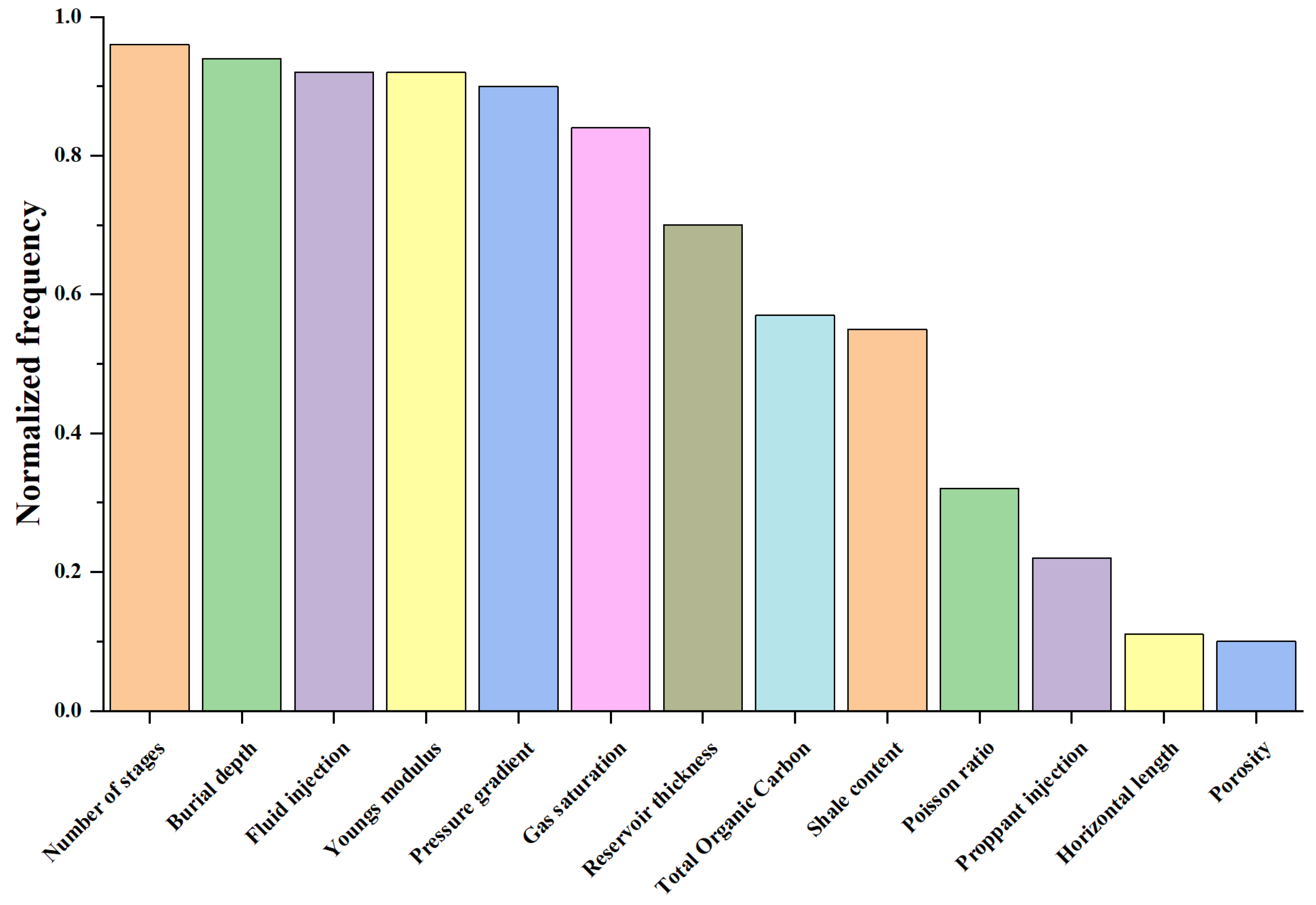
4.2.1. Feature Importance

The hyperparameter-tuning process is finished. For example, a Random Forest model is built using leaf sizes of 3, 6, 9 and 12, respectively (Figure 7). It shows the error performance after Random Forest regression using different leaf sizes. From the figure, it can be seen that the smaller the selected leaf size, the lower the model’s error rate, and the model with a leaf size of 3 has the lowest final error, indicating that the model performs better. The leaf size of 3 was determined as the final parameter.

The input variables consist of 13 relevant metrics from 3146 wells, whereas the output variables are the natural gas production of these wells. The machine learning procedure is performed by integrating the input and output variables. Figure 8 depicts the normalized frequencies of the 13 input variables, thereby highlighting the importance of the parameters in generating the predictive model. The findings indicate that fracturing fluid injection, burial depth and the number of fractured sections are the features that contribute most to tight gas production, with their normalized frequencies greater than 0.9. Young’s modulus, formation pressure, saturation, sandstone thickness and total organic carbon content are the next most influential factors, with normalized frequency greater than 0.75 but less than 0.9. Other features, including mud content, Poisson’s ratio, proppant injection volume, horizontal section length and porosity, had the least correlation, with normalized frequencies less than 0.5. These five parameters are considered to be of lesser importance because they may be directly proportional to certain more crucial values. The proportional relationship reduces their individual influence and importance in the analysis. For example, gas saturation, total organic carbon content and mud content are positively correlated with Young’s modulus. Similarly, the cumulative proppant injection volume is directly proportional to the fracturing fluid-injection volume.

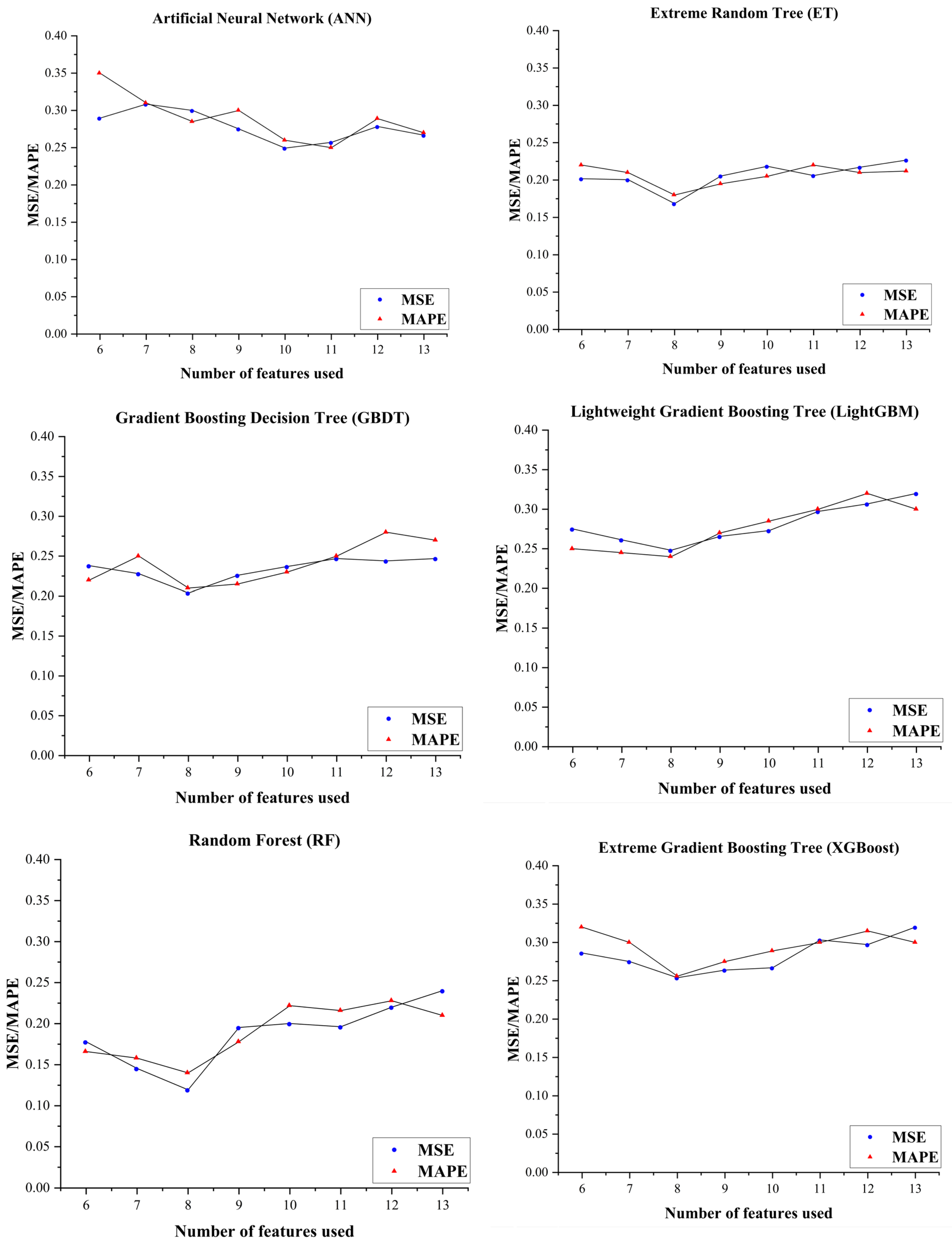
4.2.2. Comparison of Different Models

Figure 9 depicts the machine learning results obtained using the six methods, as a function of the number of parameters selected. The six algorithms consistently identified eight parameters that yielded the highest R². These parameters, including the number of fracturing sections, burial depth, fracturing fluid injection volume, Young’s modulus, formation pressure and gas saturation, are the fundamental determinants for enhancing tight gas production.

The average R² of these eight parameters across the different methods are as follows (Figure 10): 0.688 for ANN, 0.853 for ET, 0.761 for GBDT, 0.823 for XGBoost, 0.783 for LightGBM and 0.886 for RF. Additionally, the average MSEs are 0.31 for ANN, 0.17 for ET, 0.21 for GBDT, 0.19 for XGBoost, 0.23 for LightGBM and 0.19 for LightGBM. LightGBM is 0.23 and RF is 0.12. Therefore, the RF stands out as the most optimal choice. With the selected eight parameters, it has the highest R² and the lowest MSE. Therefore, the RF was ultimately selected to construct the prediction model for tight gas production capacity.

4.2.3. Prediction of Long-Term Production

The significance of the RF-based prediction model lies in its ability to predict natural gas-production rates, in terms of tight gas-production equivalents, over 12 months. Specifically, the RF-based prediction model predicts tight gas-production rates in the study area based on a prediction model of eight selected parameters (i.e., fracturing fluid injection, burial depth, number of fracturing sections, Young’s modulus, formation pressure, saturation, sandstone thickness and total organic carbon content). The inferred gas-production capacity maps for the 6-month, 12-month and 18-month durations (Figure 11a–c) exhibit a high degree of correspondence with the observed spatial production capacity (Figure 11d). This correspondence serves to validate the effectiveness and reliability of the RF-based model. This predictive model can be utilized to guide the future positioning of horizontal wells in the Montney Formation. Additionally, this approach can also be applied to other scenarios of tight gas production.

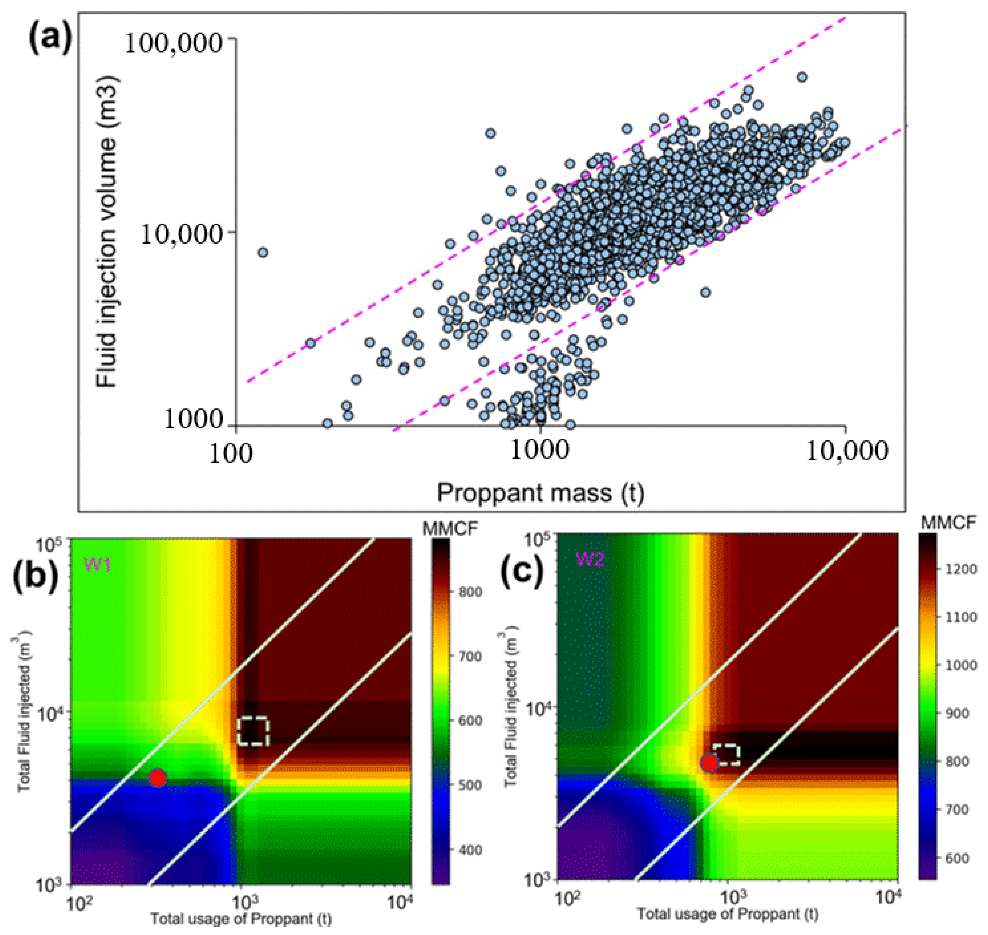
4.2.4. Optimization of Fracturing Parameters

The core aspect of this research is the optimization of fracturing parameters using the RF-based prediction model. Specifically, the fracturing fluid-injection volume and proppant mass are optimized to maximize gas productivity. Based on the relationship between fluid-injection volume and proppant mass in the studied region (Figure 12a), case studies of two test wells are conducted with the RF-based prediction model. Figure 12b,c present the details of fracturing parameter optimization for the two wells. The grey box marks the optimal range for engineering parameters corresponding to the maximum 12-month gas production. It is evident that the original fracturing parameters of Well W2 are similar to the optimal ones. The original fluid-injection volume was 4700 m³ and the proppant mass was 800 t, compared to the optimal 5300 m³ of fluid injection and 1000 t of proppant mass. Therefore, the actual 12-month production of 1150 MMCF is close to that of 1270 MMCF. In contrast, Well W1 has relatively low production due to inappropriate fracturing parameters. If the fluid injection is increased by 97.5% and the proppant mass is increased by 243.8%, the optimal gas production of W1 would be 880 MMCF (

Table 4. Optimization of fracturing parameters for two horizontal wells.

Well	Original Parameters			Optimal Parameters			Parameter Comparison
	12 Mo Prod (MMCF)	Fluid Volume (m3)	Proppant Mass (t)	12 Mo Prod (MMCF)	Fluid Volume (m3)	Proppant Mass (t)	Fluid Increment (%)	Proppant Increment (%)
W1	480	4000	320	890	7900	1100	97.5	243.8
W2	1150	4700	800	1270	5300	1000	12.8	25.0

). This work is highly significant as it determines the fracturing job scales under site-specific geological parameters of the studied region.

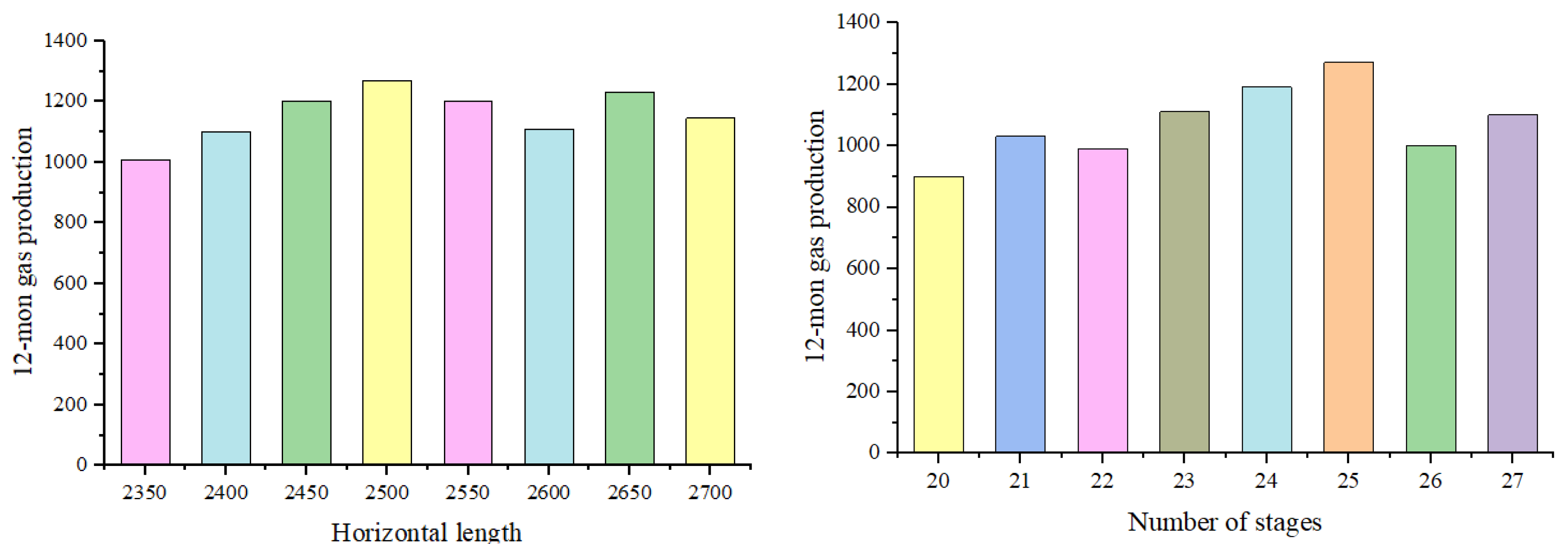
4.2.5. Sensitivity Analysis of Fracturing Parameters

By applying the fracturing parameter-optimization model and the yield-prediction model above, a fracturing parameter sensitivity analysis can be realized. Take the above Well W2 as an example to illustrate the process of this sensitivity analysis. The set of scenario parameters with the highest predicted yield is the benchmark for the fracturing parameter sensitivity analysis. In the single-factor analysis, only one parameter is altered at a time. In Figure 13, when the cumulative injection volume of the fracturing fluid is 4700 m³ and the cumulative pumping volume of proppant is 800 t, the maximum yield is attained when the number of designed fracturing sections is 18. Thus, under these fluid proppant conditions, the optimal number of fracturing sections is 18 and these scenario-specific fracturing parameters can be used as the basis for the sensitivity analysis. Furthermore, with the cumulative injection volume of fracturing fluid of 4700 m³ and the cumulative pumped-in volume of proppant of 800 t, the highest yield can be obtained when the length of the designed horizontal section is 2500 m. Therefore, under these fluid proppant conditions, the optimal horizontal section length is 2500 m.

5. Conclusions

This paper proposes a novel data-driven approach for predicting tight gas production. It effectively integrates machine learning algorithms, feature selection, production prediction and fracturing parameter optimization. First, a database of geological and engineering parameters from 3146 horizontal wells in the Montney tight gas field was collected. Second, six machine learning methods were trained to predict production performance and quantify the contribution of geological and engineering factors to production outcomes. Operational plans were optimized to maximize productivity by adjusting the fracturing fluid-injection volume and proppant mass through the optimal calculating algorithm.

(1)

The six machine learning algorithms selected eight parameters of the highest R² values. These parameters include fracturing fluid injection, burial depth, number of fractured sections, Young’s modulus, formation pressure, saturation, sandstone thickness and total organic carbon (TOC) content and emerged as the key variables for tight gas production.

(2)

After evaluating six machine learning algorithms, the Random Forest method was found to have the largest coefficient of determination, with an R² value of 0.886. A prediction model based on Random Forest was then developed to estimate tight gas productivity, which can be used to guide the well site selection for effective tight gas development.

(3)

A case study of test wells demonstrated that the model can be used for fracturing parameter sensitivity analysis. By analyzing the impact of single- or multi-factor variations on production, it enables the optimal design of single or multiple parameters. Ultimately, increasing the fracturing fluid injection by 97.5% can nearly double the natural gas production. This work has provided accurate, evidence-based suggestions for optimizing the development plan.

References

- McGlade, C.; Speirs, J.; Sorrell, S. Unconventional Gas—A Review of Regional and Global Resource Estimates. Energy 2013, 55, 571–584. [Google Scholar] [CrossRef]
- Wang, H.; Ma, F.; Tong, X.; Liu, Z.; Zhang, X.; Wu, Z.; Li, D.; Wang, B.; Xie, Y.; Yang, L. Assessment of Global Unconventional Oil and Gas Resources. Pet. Explor. Dev. 2016, 43, 925–940. [Google Scholar] [CrossRef]
- Sun, L.; Zou, C.; Jia, A.; Wei, Y.; Zhu, R.; Wu, S.; Guo, Z. Development Characteristics and Orientation of Tight Oil and Gas in China. Pet. Explor. Dev. 2019, 46, 1073–1087. [Google Scholar] [CrossRef]
- Di, C.; Wei, Y.; Wang, K.; Deng, P.; Chen, B.; Shen, L.; Chen, Z. The Impact of Pressurization-Induced Decrease of Capillary Pressure and Residual Saturation on Geological Carbon Dioxide Storage. J. Clean. Prod. 2025, 486, 144573. [Google Scholar] [CrossRef]
- Hui, G.; Chen, S.; He, Y.; Wang, H.; Gu, F. Machine Learning-Based Production Forecast for Shale Gas in Unconventional Reservoirs via Integration of Geological and Operational Factors. J. Nat. Gas Sci. Eng. 2021, 94, 104045. [Google Scholar] [CrossRef]
- Chen, J.; Wang, L.; Wang, C.; Yao, B.; Tian, Y.; Wu, Y.S. Automatic Fracture Optimization for Shale Gas Reservoirs Based on Gradient Descent Method and Reservoir Simulation. Adv. Geo-Energy Res. 2021, 5, 191–201. [Google Scholar] [CrossRef]
- Hui, G.; Chen, Z.; Schultz, R.; Chen, S.; Song, Z.; Zhang, Z.; Song, Y.; Wang, H.; Wang, M.; Gu, F. Intricate Unconventional Fracture Networks Provide Fluid Diffusion Pathways to Reactivate Pre-Existing Faults in Unconventional Reservoirs. Energy 2023, 282, 128803. [Google Scholar] [CrossRef]
- Weng, X.; Kresse, O.; Chuprakov, D.; Cohen, C.E.; Prioul, R.; Ganguly, U. Applying Complex Fracture Model and Integrated Workflow in Unconventional Reservoirs. J. Pet. Sci. Eng. 2014, 124, 468–483. [Google Scholar] [CrossRef]
- Awoleke, O.; Lane, R. Analysis of Data from the Barnett Shale Using Conventional Statistical and Virtual Intelligence Techniques. SPE Reserv. Eval. Eng. 2011, 14, 544–556. [Google Scholar] [CrossRef]
- Wang, Y.-F.; Xu, S.; Hao, F.; Liu, H.-M.; Hu, Q.-H.; Xi, K.-L.; Yang, D. Machine Learning-Based Grayscale Analyses for Lithofacies Identification of the Shahejie Formation, Bohai Bay Basin, China. Pet. Sci. 2025, 22, 42–54. [Google Scholar] [CrossRef]
- Ozowe, W.; Daramola, G.O.; Ekemezie, I.O. Recent Advances and Challenges in Gas Injection Techniques for Enhanced Oil Recovery. Magna Sci. Adv. Res. Rev. 2023, 9, 168–178. [Google Scholar] [CrossRef]
- Hui, G.; Chen, Z.; Wang, Y.; Zhang, D.; Gu, F. An Integrated Machine Learning-Based Approach to Identifying Controlling Factors of Unconventional Shale Productivity. Energy 2023, 266, 126512. [Google Scholar] [CrossRef]
- Mohammed, A.I.; Bartlett, M.; Oyeneyin, B.; Kayvantash, K.; Njuguna, J. An Application of FEA and Machine Learning for the Prediction and Optimisation of Casing Buckling and Deformation Responses in Shale Gas Wells in an In-Situ Operation. J. Nat. Gas Sci. Eng. 2021, 95, 104221. [Google Scholar] [CrossRef]
- Chen, Z.; Jiang, C. An Integrated Mass Balance Approach for Assessing Hydrocarbon Resources in a Liquid-Rich Shale Resource Play: An Example from Upper Devonian Duvernay Formation, Western Canada Sedimentary Basin. J. Earth Sci. 2020, 31, 1259–1272. [Google Scholar] [CrossRef]
- Kalantari-Dahaghi, A.; Mohaghegh, S.; Esmaili, S. Coupling Numerical Simulation and Machine Learning to Model Shale Gas Production at Different Time Resolutions. J. Nat. Gas Sci. Eng. 2015, 25, 380–392. [Google Scholar] [CrossRef]
- Tahmasebi, P.; Javadpour, F.; Sahimi, M. Data Mining and Machine Learning for Identifying Sweet Spots in Shale Reservoirs. Expert Syst. Appl. 2017, 88, 435–447. [Google Scholar] [CrossRef]
- Meng, J.; Zhou, Y.; Ye, T.; Xiao, Y.; Lu, Y.; Zheng, A.W.; Liang, B. Hybrid Data-Driven Framework for Shale Gas Production Performance Analysis via Game Theory, Machine Learning, and Optimization Approaches. Pet. Sci. 2023, 20, 277–294. [Google Scholar] [CrossRef]
- Saporetti, C.; Fonseca, D.; Oliveira, L.; Pereira, E.; Goliatt, L. Hybrid Machine Learning Models for Estimating Total Organic Carbon from Mineral Constituents in Core Samples of Shale Gas Fields. Mar. Pet. Geol. 2022, 143, 105783. [Google Scholar] [CrossRef]
- Vikara, D.; Remson, D.; Khanna, V. Machine Learning-Informed Ensemble Framework for Evaluating Shale Gas Production Potential: Case Study in the Marcellus Shale. J. Nat. Gas Sci. Eng. 2020, 84, 103679. [Google Scholar] [CrossRef]
- Mehana, M.; Guiltinan, E.; Vesselinov, V.; Middleton, R.; Hyman, J.D.; Kang, Q.; Viswanathan, H. Machine-Learning Predictions of the Shale Wells’ Performance. J. Nat. Gas Sci. Eng. 2021, 88, 103819. [Google Scholar] [CrossRef]
- Xiao, C.; Wang, G.; Zhang, Y.; Deng, Y. Machine-Learning-Based Well Production Prediction under Geological and Hydraulic Fracture Parameters Uncertainty for Unconventional Shale Gas Reservoirs. J. Nat. Gas Sci. Eng. 2022, 106, 104762. [Google Scholar] [CrossRef]
- Yi, J.; Qi, Z.; Li, X.; Liu, H.; Zhou, W. Spatial Correlation-Based Machine Learning Framework for Evaluating Shale Gas Production Potential: A Case Study in Southern Sichuan Basin, China. Appl. Energy 2024, 357, 122483. [Google Scholar] [CrossRef]
- Bachu, S.; Burwash, R.A. Regional-Scale Analysis of the Geothermal Regime in the Western Canada Sedimentary Basin. Geothermics 1991, 20, 387–407. [Google Scholar] [CrossRef]
- González, P.; Furlong, C.; Gingras, M.; Playter, T.; Zonneveld, J. Depositional Framework and Trace Fossil Assemblages of the Lower Triassic Montney Formation, Northeastern British Columbia, Western Canada Sedimentary Basin. Mar. Pet. Geol. 2022, 143, 105822. [Google Scholar] [CrossRef]
- Hui, G.; Chen, S.; Gu, F. Strike-Slip Fault Reactivation Triggered by Hydraulic-Natural Fracture Propagation during Fracturing Stimulations near Clark Lake, Alberta. Energy Fuels 2024, 38, 18547–18555. [Google Scholar] [CrossRef]
- Egbobawaye, E. Sedimentology and Ichnology of Upper Montney Formation Tight Gas Reservoir, Northeastern British Columbia, Western Canada Sedimentary Basin. IJG 2016, 07, 1357–1411. [Google Scholar] [CrossRef]
- Bao, P.; Hui, G.; Hu, Y.; Song, R.; Chen, Z.; Zhang, K.; Pi, Z.; Li, Y.; Ge, C.; Yao, F.; et al. Comprehensive Characterization of Hydraulic Fracture Propagations and Prevention of Pre-existing Fault Failure in Duvernay Shale Reservoirs. Eng. Fail. Anal. 2025, 173, 109461. [Google Scholar] [CrossRef]
- Hui, G.; Yao, F.; Pi, Z.; Bao, P.; Wang, W.; Wang, M.; Wang, H.; Gu, F. Tight Gas Production Prediction in the Southern Montney Play Using Machine Learning Approaches. In Proceedings of the SPE Canadian Energy Technology Conference and Exhibition, Calgary, AB, Canada, 13 March 2024; p. D011S009R001. [Google Scholar]
- Fang, M.; Shi, H.; Li, H.; Liu, T. Application of Machine Learning for Productivity Prediction in Tight Gas Reservoirs. Energies 2024, 17, 1916. [Google Scholar] [CrossRef]
- Mao, S.; Chen, B.; Malki, M.; Chen, F.; Morales, M.; Ma, Z.; Mehana, M. Efficient Prediction of Hydrogen Storage Performance in Depleted Gas Reservoirs Using Machine Learning. Appl. Energy 2024, 361, 122914. [Google Scholar] [CrossRef]
- LeCun, Y.; Bengio, Y.; Hinton, G. Deep Learning. Nature 2015, 521, 436–444. [Google Scholar] [CrossRef]
- Hui, G.; Chen, Z.; Wang, H.; Song, Z.; Wang, S.; Zhang, H.; Zhang, D.M.; Gu, F. A Machine Learning-Based Study of Multifactor Susceptibility and Risk Control of Induced Seismicity in Unconventional Reservoirs. Pet. Sci. 2023, 20, 2232–2243. [Google Scholar] [CrossRef]
- Deng, Y.; Wang, W.; Su, Y.; Sun, S.; Zhuang, X. An Unsupervised Machine Learning Based Double Sweet Spots Classification and Evaluation Method for Tight Reservoirs. J. Energy Res. Technol. 2023, 145, 072602. [Google Scholar] [CrossRef]
- Pawley, S.; Schultz, R.; Playter, T.; Corlett, H.; Shipman, T.; Lyster, S.; Hauck, T. The Geological Susceptibility of Induced Earthquakes in the Duvernay Play. Geophys. Res. Lett. 2018, 45, 1786–1793. [Google Scholar] [CrossRef]
- Brantson, E.T.; Ju, B.; Omisore, B.O.; Wu, D.; Selase, A.E.; Liu, N. Development of Machine Learning Predictive Models for History Matching Tight Gas Carbonate Reservoir Production Profiles. J. Geophys. Eng. 2018, 15, 2235–2251. [Google Scholar] [CrossRef]
- Zou, C.; Yang, Z.; He, D.; Wei, Y.; Li, J.; Jia, A.; Chen, J.; Zhao, Q.; Li, Y.; Li, J.; et al. Theory, Technology and Prospects of Conventional and Unconventional Natural Gas. Pet. Explor. Dev. 2018, 45, 604–618. [Google Scholar] [CrossRef]
- Song, N.; Li, S.; Zeng, B.; Duan, R.; Yang, Y. A Novel Grey Prediction Model with Four-Parameter and Its Application to Forecast Natural Gas Production in China. Eng. Appl. Artif. Intell. 2024, 133, 108431. [Google Scholar] [CrossRef]
- Zhang, Z.; Tang, J.; Zhang, J.; Meng, S.; Li, J. Modeling of Scale-Dependent Perforation Geometrical Fracture Growth in Naturally Layered Media. Eng. Geol. 2024, 336, 107499. [Google Scholar] [CrossRef]
- Song, R.; Liu, J.; Yang, C.; Sun, S. Study on the Multiphase Heat and Mass Transfer Mechanism in the Dissociation of Methane Hydrate in Reconstructed Real-Shape Porous Sediments. Energy 2022, 254, 124421. [Google Scholar] [CrossRef]
- Su, X.; Zhou, D.; Wang, H.; Xu, J. Research on the Scaling Mechanism and Countermeasures of Tight Sandstone Gas Reservoirs Based on Machine Learning. Processes 2024, 12, 527. [Google Scholar] [CrossRef]
- Hui, G.; Chen, Z.; Chen, S.; Gu, F. Hydraulic Fracturing-Induced Seismicity Characterization through Coupled Modeling of Stress and Fracture-Fault Systems. Adv. Geo-Energy Res. 2022, 6, 269–270. [Google Scholar] [CrossRef]
- Cao, L.; Jiang, F.; Chen, Z.; Gao, Y.; Huo, L.; Chen, D. Data-Driven Interpretable Machine Learning for Prediction of Porosity and Permeability of Tight Sandstone Reservoir. Adv. Geo-Energy Res. 2025, 16, 21–35. [Google Scholar] [CrossRef]
- Xie, C.; Du, S.; Wang, J.; Lao, J.; Song, H. Intelligent Modeling with Physics-Informed Machine Learning for Petroleum Engineering Problems. Adv. Geo-Energy Res. 2023, 8, 71–75. [Google Scholar] [CrossRef]
- Omidkar, A.; Alagumalai, A.; Li, Z.; Song, H. Machine Learning Assisted Techno-Economic and Life Cycle Assessment of Organic Solid Waste Upgrading under Natural Gas. Appl. Energy 2024, 355, 122321. [Google Scholar] [CrossRef]
- Wang, S.; Chen, S. Insights to Fracture Stimulation Design in Unconventional Reservoirs Based on Machine Learning Modeling. J. Pet. Sci. Eng. 2019, 174, 682–695. [Google Scholar] [CrossRef]
- Naghizadeh, A.; Jafari, S.; Norouzi-Apourvari, S.; Schaffie, M.; Hemmati-Sarapardeh, A. Multi-Objective Optimization of Water-Alternating Flue Gas Process Using Machine Learning and Nature-Inspired Algorithms in a Real Geological Field. Energy 2024, 293, 130413. [Google Scholar] [CrossRef]
- Liu, L.; Kang, W.; Wang, Y.; Zeng, L. Design of Tool Wear Monitoring System in Bone Material Drilling Process. Coatings 2024, 14, 812. [Google Scholar] [CrossRef]
- Genuer, R.; Poggi, J.; Tuleau-Malot, C.; Villa-Vialaneix, N. Random Forests for Big Data. Big Data Res. 2017, 9, 28–46. [Google Scholar] [CrossRef]
- Bakouregui, A.; Mohamed, H.; Yahia, A.; Benmokrane, B. Explainable Extreme Gradient Boosting Tree-Based Prediction of Load-Carrying Capacity of FRP-RC Columns. Eng. Struct. 2021, 245, 112836. [Google Scholar] [CrossRef]
- Lawal, A.; Yang, Y.; He, H.; Baisa, N.L. Machine Learning in Oil and Gas Exploration: A Review. IEEE Access 2024, 12, 19035–19058. [Google Scholar] [CrossRef]
- Tang, J.; Zhang, Z.; Xie, J.; Meng, S.; Xu, J.; Ehlig-Economides, C.; Liu, H. Re-Evaluation of CO2 Storage Capacity of Depleted Fractured-Vuggy Carbonate Reservoir. Innov. Energy 2024, 1, 100019-1–100019-11. [Google Scholar] [CrossRef]
- Wang, Z.-Y.; Lu, S.-F.; Zhou, N.-W.; Liu, Y.-C.; Lin, L.-M.; Shang, Y.-X.; Wang, J.; Xiao, G.-S. Complementary Testing and Machine Learning Techniques for the Characterization and Prediction of Middle Permian Tight Gas Sandstone Reservoir Quality in the Northeastern Ordos Basin, China. Pet. Sci. 2024, 21, 2946–2968. [Google Scholar] [CrossRef]
- Hu, X.; Meng, Q.; Guo, F.; Xie, J.; Hasi, E.; Wang, H.; Zhao, Y.; Wang, L.; Li, P.; Zhu, L.; et al. Deep Learning Algorithm-Enabled Sediment Characterization Techniques to Determination of Water Saturation for Tight Gas Carbonate Reservoirs in Bohai Bay Basin, China. Sci. Rep. 2024, 14, 12179. [Google Scholar] [CrossRef] [PubMed]
- Liu, B.; Li, C. Mining and Analysis of Production Characteristics Data of Tight Gas Reservoirs. Processes 2023, 11, 3159. [Google Scholar] [CrossRef]
- Zhao, X.; Chen, X.; Chen, W.; Liu, M.; Yao, Y.; Wang, H.; Zhang, H.; Yao, G. Quantitative Classification and Prediction of Diagenetic Facies in Tight Gas Sandstone Reservoirs via Unsupervised and Supervised Machine Learning Models: Ledong Area, Yinggehai Basin. Nat. Resour. Res. 2023, 32, 2685–2710. [Google Scholar] [CrossRef]