An Efficient Scheduling Method in Supply Chain Logistics Based on Network Flow

Abstract

In the evolving digital landscape, network flow models have become integral to various sectors, including supply chain management. This research develops a robust network flow model for semiconductor wafer supply chains, optimizing resource allocation and addressing maximum flow challenges in production and logistics. The model incorporates the stochastic nature of wafer batch transfers and employs a dual-layer optimization framework to reduce variability and exceedance probabilities in finished goods. Empirical comparisons reveal significant enhancements in cost efficiency, productivity, and resource utilization, with a 20% reduction in time and production costs and a 10% increase in transportation and storage capacities. The model’s efficacy is underscored by a 15% decrease in transportation time and a 6700 kg increase in total capacity, demonstrating its capability to resolve logistical bottlenecks in semiconductor manufacturing. This study concludes that network flow models are a potent tool for optimizing supply chain logistics and offer a 23% improvement in resource utilization along with a 13% boost in accuracy. The findings provide valuable insights for supply chain logistics optimization.

1. Introduction

In the 21st century, the rapid development of electronic technology and information technology has had a huge impact on social production, and semiconductor wafer manufacturing is a key area of concern. Semiconductor wafers, as the core material of the modern electronics industry, are widely used in electronic devices and applications such as computers, communications, consumer electronics, and automobiles [1]. The production and transportation of wafers are crucial links in the manufacturing process, and effective transportation management can improve production efficiency and reduce costs [2,3]. However, wafer transportation involves a complex logistics network and coordination of multiple nodes [4], so optimizing the transportation process of wafers is of great significance. This study employs a network flow model to enhance production logistics efficiency in wafer manufacturing by reducing errors, minimizing losses, and improving security. These advantages have gradually become the focus of research in the wafer manufacturing industry and among domestic and foreign scholars [5].

The network flow model is a mathematical model used to describe the flow of resources or information transmission in a network structure. It involves finding the maximum flow path from one specific node to another in the network [6]. Despite the extensive research on network flow models in supply chain logistics scheduling, the existing literature still exhibits significant limitations. For instance, the adaptive network flow model proposed by Bin et al. [7] focuses on network traffic anomaly detection and does not address the uncertainty in dynamic scheduling for manufacturing. Although Feng et al. [8] applied network flow models to logistics task allocation, their model fails to adequately consider the stochastic nature of wafer lot transfer probability (WLTP) and its impact on work-in-progress (WIP) fluctuations in semiconductor manufacturing. Similarly, Bohacs et al. [9] attempted to integrate scheduling with energy efficiency, but their single-layer optimization framework struggles to handle multi-objective conflicts in complex production environments. Likewise, Qinyue et al. [10] improved network flow identification algorithms, yet their research is confined to static path planning, lacking dynamic adjustments for real-time transportation capacities and path selection. While these studies have advanced the development of network flow theory, none have proposed a systematic solution tailored to the unique requirements of semiconductor wafer transportation, such as high-precision scheduling [11,12], multi-node coordination [13], and stochasticity suppression [14]. Therefore, the research question of this article is to optimize the rail layout of semiconductor wafer transportation based on the network flow model, consider the matching methods of network flow models for different scheduling tasks, and propose a transportation path optimization strategy based on a multi-objective accurate algorithm in network flow models. Previous studies have mainly concentrated on max flow, min-cost flow, and maximum bipartite matching problems in network flow models, with insufficient attention to the unique challenges in semiconductor wafer manufacturing and transportation. This process involves a complex logistics network and multi-node coordination, requiring a comprehensive approach to transport route optimization, vehicle configuration, and task matching, areas where existing research falls short.

Moreover, prior research has room for improvement in handling uncertainties in semiconductor wafer manufacturing and transportation. The probability of wafer lot transfers in manufacturing is uncertain, affecting production scheduling and logistics. Although robust optimization methods have been introduced, there is still a need for optimization in model building and algorithm design specific to semiconductor wafer transportation.

To solve the above problems, this article deepens and extends previous research. A two-level optimization framework is proposed to handle the uncertainty in wafer lot transfer probabilities, enhancing model robustness and stability. The network flow model is applied to the specific scenario of semiconductor wafer manufacturing and transportation. By defining warehouse nodes and edge capacities, it optimizes transport routes and vehicle allocation to reduce transport distance and boost efficiency. The model’s effectiveness is also verified through experiments, comparing pre- and post-optimization metrics such as cost, completion time, and production efficiency and showing the practical benefits of the network flow model in optimizing semiconductor wafer manufacturing and transportation. This study develops a logistics management system (LMS) for optimizing semiconductor wafer transportation using a network flow model [15,16,17], thereby enhancing the accuracy and reliability of transportation paths and integrating the transportation process more efficiently into production logistics scheduling. By defining warehouse nodes and edge capacities, the proposed model interconnects multiple transport paths, optimizes the loading and unloading ports of storage warehouses as output and input ports, and minimizes the transportation distance of carriers while rationalizing the allocation of maximum transport path capacities. These enhancements collectively improve the efficiency of semiconductor wafer transport systems. Furthermore, this research introduces a dual-layer robust production capacity planning model to address uncertainties in wafer lot transfer probabilities (WLTPs). The lower layer evaluates average work-in-process (WIP) levels using an open queuing network model [18], analyzing WIP fluctuations under varying numbers of carriers, while the upper layer determines the optimal carrier configuration to minimize maximum WIP fluctuations and ensure that WIP levels do not exceed a predefined upper limit probability. The overarching objective [19] is to validate the effectiveness of the network flow model in optimizing semiconductor wafer transport efficiency through comparative analysis of optimized and pre-optimized experimental data, and to demonstrate its potential for enhancing production and logistics scheduling within the supply chain. Based on these objectives, this study addresses the following research questions: How can the proposed network flow model optimize the transportation layout of semiconductor wafer transportation to improve efficiency and reduce costs? How does the dual-layer optimization framework effectively address uncertainties in wafer lot transfer probabilities and stabilize WIP levels? What are the impacts of the proposed model on production logistics scheduling, resource utilization, and overall supply chain performance?

2. Building a Network Flow Model

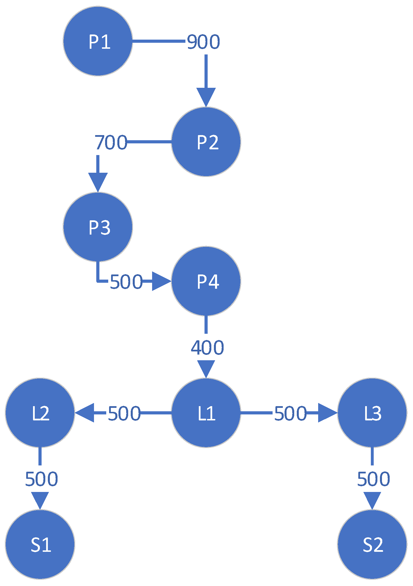
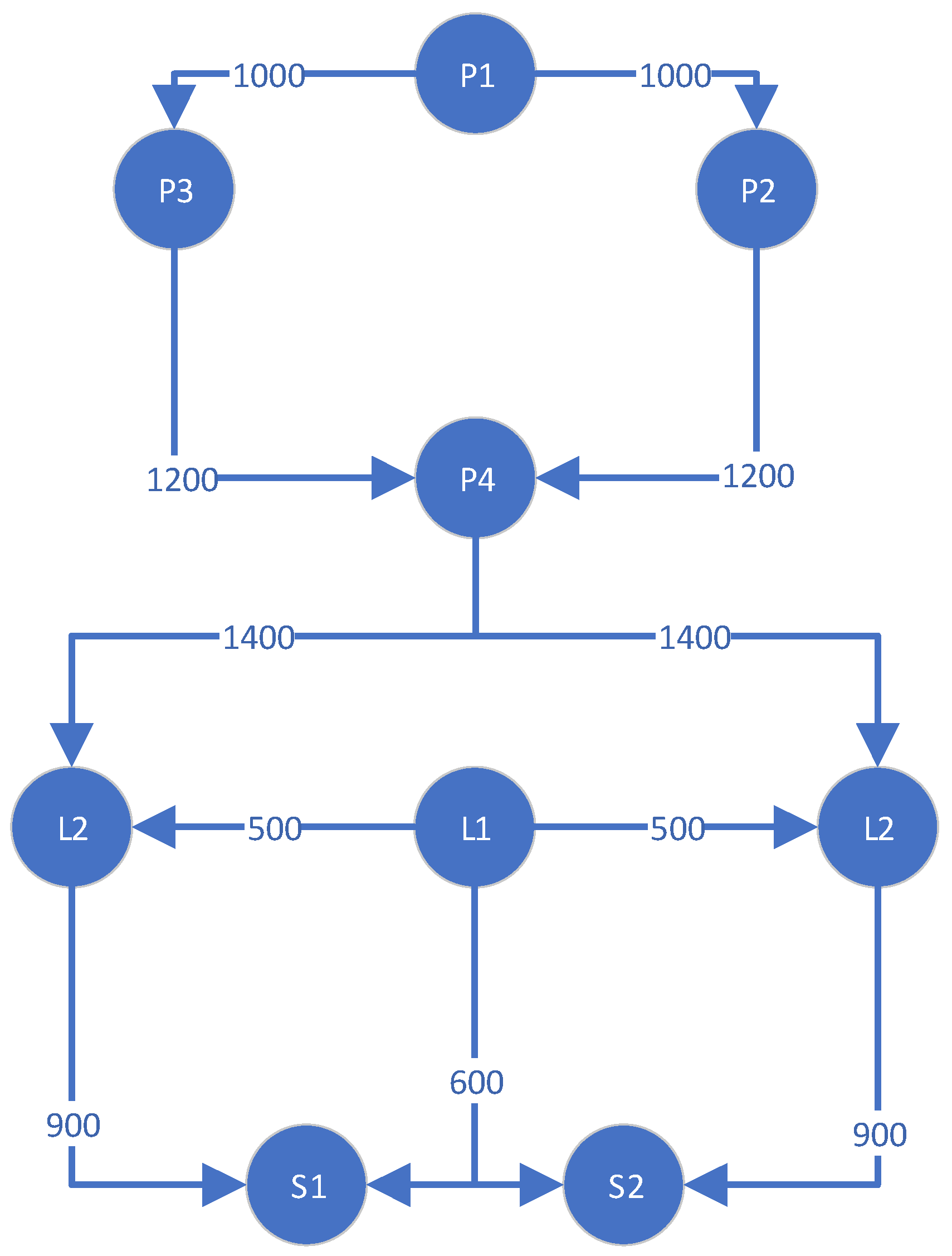
2.1. Specific Problem Description

In semiconductor manufacturing, the uncertainty in wafer lot transfer poses challenges to production scheduling, particularly in managing the transportation of wafer lots between different production areas [20]. This study aims to optimize production logistics scheduling in the supply chain using a network flow model to enhance the efficiency and robustness of the semiconductor wafer transport system.

To address the uncertainty of wafer lot transfer probability (WLTP), we introduce a two-tier robust production capacity planning model. The lower-tier model focuses on analyzing work-in-process (WIP) level fluctuations given a fixed number of vehicles and assesses system stability under WLTP variations. The upper-tier model aims to determine the optimal vehicle allocation to minimize WIP level fluctuations and ensure that the probability of WIP exceeding a predefined upper limit is minimized. The overall architecture is illustrated in Figure 1.

The lower-tier model employs an open queuing network model to evaluate the average WIP level in the automated material handling system (AMHS). This model is based on key variables including the following:

(1)

WLTP: probability of wafer lot transfer between different production areas;

(2)

WIP: average number of wafer lots in process within the system;

(3)

Vehicle count: number of automated vehicles for wafer transportation.

The model interconnects multiple transport paths by defining warehouse nodes and edge capacities and optimizing warehouse loading and unloading ports as input and output points. This design of the network flow model helps reduce the transport distance of transport carts and rationalize the maximum capacity allocation of transport paths, thereby enhancing the efficiency of the transport system.

The upper-tier model solves a bi-objective optimization problem by determining the optimal vehicle allocation that minimizes fluctuations in WIP levels while ensuring that WIP does not exceed a defined limit. Considering the impact of WLTP uncertainty on the stability of WIP levels, the vehicle count is adjusted to optimize the overall performance of the production logistics scheduling system.

Quantifying the impact of WLTP uncertainty on WIP level fluctuations is performed in the lower-tier model under a given number of vehicles. The upper-tier model uses bi-objective optimization methods to find the best vehicle allocation strategy while meeting the probability constraints of the WIP upper limit. This two-tier optimization framework effectively enhances system robustness and efficiency, enabling the semiconductor wafer transport system to operate stably in complex production environments.

2.2. Mathematical Model Formulation

In semiconductor manufacturing, the uncertainty of wafer lot transfer probabilities (WLTPs) has a significant impact on the average work-in-progress (WIP) level [21]. In order to optimize production capacity, a robust production plan is required, especially to determine the optimal number of vehicles in the automated material handling system (AMHS) so that the WIP level can be kept stable even when the WLTPs fluctuate. To this end, an open queuing network model based on the M/M/1 system principle is constructed to evaluate the WIP level, and a two-level optimization model is introduced.

At the bottom level, the goal of the model is to maximize the directional derivative of the WIP level with respect to WLTPs, that is, the degree of fluctuation of the WIP level, for a given number of vehicles. Through analytical derivation, the following conclusions can be proved: ${\left.{\displaystyle \frac{\partial W}{\partial p_i}}\right|}_{p_c}$ is $p_0$, a monotonically decreasing function, and is $p_i$ a monotonically increasing function, where $W(p,c)$ is the average WIP level under a given number of vehicles $c$ and transition probability $p$. Additionally, ${\displaystyle \frac{\partial \mathrm{W}}{\partial {\mathrm{p}}_{\mathrm{i}}}}>0$ holds when the transition probability ${\mathrm{p}}_{\mathrm{i}}$ varies within the range $0\le {\mathrm{p}}_{\mathrm{i}}\le 1.$

At the upper level, the goal is to determine the vehicle combination that minimizes the $c^{\ast }$ maximum directional derivative and the probability that the WIP level exceeds a specified upper limit $W^{\ast }$. It is necessary to find the one where $V^{\ast }(p^{\ast },x^{\ast }|c)$ minimizes $c$, where $V^{\ast }(p^{\ast },x^{\ast }|c)$ is the worst-case WIP level volatility, that is, when $p=p^{\ast }$ and is in the direction of the mathematical expectation where the WIP level grows fastest $x=x^{\ast }$.

To describe this optimization problem mathematically, the following key variables are introduced:

(1)

WLTP vector $p=(p_0,p_1,\dots ,p_n{)}^T$, where $p_i$ represents the probability of a wafer being transferred from one production area to another;

(2)

WIP level $W(p,c)$, which is the average WIP level given the number of vehicles $c$ and transition probability $p$;

(3)

Directional derivative $V(p,x|c)$, which is the rate of change of the WIP level with respect to WLTPs;

(4)

The number of vehicles $c$, that is, the total number of vehicles used to transport wafers in the AMHS;

(5)

Maximum WIP Fluctuation $V^{\ast }(p^{\ast },x^{\ast }|c)$, which is the maximum change in the WIP level under the worst-case scenario;

(6)

Upper limit $W^{\ast }$, which is the upper limit of the allowed WIP level.

2.2.1. Notation and Assumptions

Sets and indices include the following:

• $\mathcal{N}$: set of production nodes (e.g., processing area ${\mathrm{P}}_1$, inspection area ${\mathrm{L}}_1$, and warehouse ${\mathrm{S}}_1$);
• $\mathcal{E}$: set of transportation paths, where $(\mathrm{i},\mathrm{j})\in \mathcal{E}$ denotes a feasible path from node $\mathrm{i}$ to $\mathrm{j}$;
• $\mathrm{k}\in \{1,\dots ,\mathrm{K}\}$: index of AGV types (classified by load capacity and speed).

Parameters include the following:

• ${\mathrm{C}}_{\mathrm{m}\mathrm{a}\mathrm{x}}$: maximum number of AGVs that the system can accommodate;
• ${\mathrm{W}}^{\mathrm{*}}$: upper limit of the allowed work-in-process (WIP) level at each node;
• ${\mathrm{Q}}_{\mathrm{i}\mathrm{j}}$: maximum transportation capacity of path $(\mathrm{i},\mathrm{j})$ (in wafer lots);
• ${\mathsf{\lambda }}_{\mathrm{i}}$: external wafer arrival rate at node $\mathrm{i}$ (Poisson-distributed);
• ${\mathsf{\mu }}_{\mathrm{i}}$: service rate at node $\mathrm{i}$ (exponentially distributed).

Decision Variables include the following:

Upper-level integer variables include the following:

• ${\mathrm{c}}_{\mathrm{k}}\in {\mathrm{Z}}^{+}$: the number of type-$\mathrm{k}$ AGVs allocated;
• ${\mathrm{y}}_{\mathrm{i}\mathrm{j}}\in \left\{\mathrm{0,1}\right\}$: binary path selection variable (${\mathrm{y}}_{\mathrm{i}\mathrm{j}}=1$ if path $(\mathrm{i},\mathrm{j})$ is activated).

Lower-level continuous variables include the following:

• ${\mathrm{p}}_{\mathrm{i}\mathrm{j}}\in \left[\mathrm{0,1}\right]$: probability of wafer transfer from node $\mathrm{i}$ to $\mathrm{j}$ (WLTP);
• ${\mathrm{x}}_{\mathrm{i}\mathrm{j}}^{\mathrm{k}}\ge 0$: transportation volume of type-$\mathrm{k}$ AGVs on path $(\mathrm{i},\mathrm{j})$;
• ${\mathrm{W}}_{\mathrm{i}}\ge 0$: average WIP level at node $\mathrm{i}$.

Assumptions include the following:

(1)

AGVs operate without failure and tasks are executed sequentially;

(2)

The transportation time is linearly proportional to the distance, with AGVs moving at constant speeds;

(3)

Wafer loading/unloading times are fixed, and equipment switching costs are negligible.

2.2.2. Lower-Level Model: WLTP Allocation and WIP Sensitivity Analysis

The objective of this study is to determine the WLTP probabilities that maximize work-in-process (WIP) fluctuations for a fixed automated guided vehicle (AGV) configuration [22], with the aim of evaluating system robustness under worst-case uncertainty.

$$s.\mathrm{t}.{\sum }_{\mathrm{i}=1}^{\mathrm{n}} {\mathrm{p}}_{\mathrm{i}}=1,0\le {\mathrm{p}}_{\mathrm{i}}\le 1$$

Constraints include the following:

(a)

WLTP probability normalization:

$${\sum }_{\mathrm{j}\in {\mathcal{N}}_{\mathrm{i}}} {\mathrm{p}}_{\mathrm{i}\mathrm{j}}=1\forall \mathrm{i}\in \mathcal{N}$$

This constraint ensures that the sum of all wafer lot transfer probabilities (WLTPs) from a given node equals 1, guaranteeing a valid probability distribution. Additionally, each WLTP value $\left(p_i\right)$ is bounded between 0 and 1 to reflect realistic transfer likelihoods, where $p_i=0$ indicates no transfer and $p_i=1$ denotes deterministic transfer.

(b)

Path capacity constraints:

$${\sum }_{\mathrm{k}=1}^{\mathrm{K}} {\mathrm{x}}_{\mathrm{i}\mathrm{j}}^{\mathrm{k}}\le {\mathrm{Q}}_{\mathrm{i}\mathrm{j}}\cdot {\mathrm{y}}_{\mathrm{i}\mathrm{j}}\forall (\mathrm{i},\mathrm{j})\in \mathcal{E}$$

The total transportation volume $\left({\mathrm{x}}_{\mathrm{i}\mathrm{j}}^{\mathrm{k}}\right)$ on path $(\mathrm{i},\mathrm{j})$ must not exceed its maximum capacity (${\mathrm{Q}}_{\mathrm{i}\mathrm{j}}$). The binary variable ${\mathrm{y}}_{\mathrm{i}\mathrm{j}}$ enforces that no goods flow through inactive paths (${\mathrm{y}}_{\mathrm{i}\mathrm{j}}=0$), ensuring that only selected paths contribute to logistics operations.

(c)

AGV task assignment:

$${\sum }_{(\mathrm{i},\mathrm{j})\in \mathcal{E}} {\mathrm{x}}_{\mathrm{i}\mathrm{j}}^{\mathrm{k}}\le {\mathsf{\eta }}_{\mathrm{k}}\cdot {\mathrm{c}}_{\mathrm{k}}\forall \mathrm{k}$$

The workload assigned to type-$\mathrm{k}$ AGVs $\left({\mathrm{x}}_{\mathrm{i}\mathrm{j}}^{\mathrm{k}}\right)$ is constrained by their total capacity, calculated as the product of their fleet size $\left({\mathrm{c}}_{\mathrm{k}}\right)$ and per-vehicle capacity $\left({\mathsf{\eta }}_{\mathrm{k}}\right)$. This prevents overloading and ensures equitable task distributions across AGV types.

(d)

WIP dynamic balance:

$${\mathrm{W}}_{\mathrm{i}}={\displaystyle \frac{{\mathsf{\lambda }}_{\mathrm{i}}+{\sum }_{\mathrm{j}\in \mathcal{N}} {\mathrm{p}}_{\mathrm{j}\mathrm{i}}{\mathsf{\lambda }}_{\mathrm{j}}}{{\mathsf{\mu }}_{\mathrm{i}}-\left({\mathsf{\lambda }}_{\mathrm{i}}+{\sum }_{\mathrm{j}\in \mathcal{N}} {\mathrm{p}}_{\mathrm{j}\mathrm{i}}{\mathsf{\lambda }}_{\mathrm{j}}\right)}}$$

This equation models the steady-state work-in-process (WIP) level at node $\mathrm{i}$ using an open queueing network. It balances external wafer arrivals $\left({\mathsf{\lambda }}_{\mathrm{i}}\right)$ and internal transfers (${\mathrm{p}}_{\mathrm{j}\mathrm{i}}{\mathsf{\lambda }}_{\mathrm{j}}$) against the node’s service rate $\left({\mathsf{\mu }}_{\mathrm{i}}\right)$, ensuring system stability $\left({\mathsf{\mu }}_{\mathrm{i}}>{\mathsf{\lambda }}_{\mathrm{i}}+\sum {\mathrm{p}}_{\mathrm{j}\mathrm{i}}{\mathsf{\lambda }}_{\mathrm{j}}\right)$.

To quantify the impact of WLTP variations on WIP stability, we derive the sensitivity by computing the partial derivative of ${\mathrm{W}}_{\mathrm{i}}$ with respect to ${\mathrm{p}}_{\mathrm{i}\mathrm{j}}$: ${\displaystyle \frac{\partial {\mathrm{W}}_{\mathrm{i}}}{\partial {\mathrm{p}}_{\mathrm{i}\mathrm{j}}}}={\displaystyle \frac{{\mathsf{\mu }}_{\mathrm{i}}{\mathsf{\lambda }}_{\mathrm{j}}}{{\left({\mathsf{\mu }}_{\mathrm{i}}-{\mathsf{\lambda }}_{\mathrm{i}}-{\sum }_{\mathrm{j}} {\mathrm{p}}_{\mathrm{j}\mathrm{i}}{\mathsf{\lambda }}_{\mathrm{j}}\right)}^2}}$. This analysis provides insight into how changes in WLTPs influence the overall system stability.

Proof. 

Let ${\mathsf{\Lambda }}_{\mathrm{i}}={\mathsf{\lambda }}_{\mathrm{i}}+{\sum }_{\mathrm{j}} {\mathrm{p}}_{\mathrm{j}\mathrm{i}}{\mathsf{\lambda }}_{\mathrm{j}}$. From Equation (5),

$${\mathrm{W}}_{\mathrm{i}}={\displaystyle \frac{{\mathsf{\Lambda }}_{\mathrm{i}}}{{\mathsf{\mu }}_{\mathrm{i}}-{\mathsf{\Lambda }}_{\mathrm{i}}}}$$

Taking the derivative with respect to ${\mathrm{p}}_{\mathrm{i}\mathrm{j}}$:

$${\displaystyle \frac{\partial {\mathrm{W}}_{\mathrm{i}}}{\partial {\mathrm{p}}_{\mathrm{i}\mathrm{j}}}}={\displaystyle \frac{\partial }{\partial {\mathrm{p}}_{\mathrm{i}\mathrm{j}}}}\left({\displaystyle \frac{{\mathsf{\Lambda }}_{\mathrm{i}}}{{\mathsf{\mu }}_{\mathrm{i}}-{\mathsf{\Lambda }}_{\mathrm{i}}}}\right)={\displaystyle \frac{{\mathsf{\lambda }}_{\mathrm{j}}\left({\mathsf{\mu }}_{\mathrm{i}}-{\mathsf{\Lambda }}_{\mathrm{i}}\right)+{\mathsf{\Lambda }}_{\mathrm{i}}{\mathsf{\lambda }}_{\mathrm{j}}}{{\left({\mathsf{\mu }}_{\mathrm{i}}-{\mathsf{\Lambda }}_{\mathrm{i}}\right)}^2}}={\displaystyle \frac{{\mathsf{\mu }}_{\mathrm{i}}{\mathsf{\lambda }}_{\mathrm{j}}}{{\left({\mathsf{\mu }}_{\mathrm{i}}-{\mathsf{\Lambda }}_{\mathrm{i}}\right)}^2}}$$

This result confirms that increasing ${\mathrm{p}}_{\mathrm{i}\mathrm{j}}$ elevates ${\mathrm{W}}_{\mathrm{i}}$, highlighting the model’s capability to capture WLTP-induced instability. □

2.2.3. Upper-Level Model: AGV Configuration and Path Selection

The objective of this research is to minimize total operational costs and work-in-process (WIP) fluctuations while satisfying WIP and capacity constraints.

Objective function:

$${\mathrm{m}\mathrm{i}\mathrm{n}}_{\mathrm{c},\mathrm{y}} [\underset{\mathrm{Transportation}\mathrm{Cost}}{\underbrace{{\sum }_{(\mathrm{i},\mathrm{j})\in \mathcal{E}} {\sum }_{\mathrm{k}=1}^{\mathrm{K}} {\mathsf{\alpha }}_{\mathrm{k}}{\mathrm{T}}_{\mathrm{i}\mathrm{j}}{\mathrm{x}}_{\mathrm{i}\mathrm{j}}^{\mathrm{k}}}}+\underset{\mathrm{Inventory}\mathrm{Cost}}{\underbrace{\mathsf{\beta }{\sum }_{\mathrm{i}\in \mathcal{N}} {\mathrm{W}}_{\mathrm{i}}}}+\underset{\mathrm{Fluctuation}\mathrm{Penalty}}{\underbrace{\mathsf{\gamma }{\sum }_{\mathrm{i}\in \mathcal{N}} \left|{\mathrm{W}}_{\mathrm{i}}-\stackrel{\mathrm{‾}}{\mathrm{W}}\right|}}]$$

where

${\mathsf{\alpha }}_{\mathrm{k}}$ is the unit time cost for type-$\mathrm{k}$ AGVs;

$\mathsf{\beta }$ is the unit WIP holding cost;

$\mathsf{\gamma }$ is the penalty coefficient for WIP deviations;

$\stackrel{\mathrm{‾}}{\mathrm{W}}={\displaystyle \frac{1}{\left|\mathrm{N}\right|}}{\sum }_{\mathrm{i}} {\mathrm{W}}_{\mathrm{i}}$ is the average WIP level.

Constraints include the following:

(e)

AGV fleet size limit:

$${\sum }_{\mathrm{k}=1}^{\mathrm{K}} {\mathrm{c}}_{\mathrm{k}}\le {\mathrm{C}}_{\mathrm{m}\mathrm{a}\mathrm{x}}$$

The total number of AGVs allocated across all types $\left({\mathrm{c}}_{\mathrm{k}}\right)$ must not exceed the system’s maximum allowable fleet size (${\mathrm{C}}_{\mathrm{m}\mathrm{a}\mathrm{x}}$). This reflects physical space constraints and budgetary limitations, preventing over-investment in vehicles.

(f)

WIP upper bound:

$${\mathrm{W}}_{\mathrm{i}}\le {\mathrm{W}}^{\mathrm{*}}\forall \mathrm{i}\in \mathrm{N}$$

The WIP level at each node $\mathrm{i}$ is capped at a predefined threshold $\left({\mathrm{W}}^{\mathrm{*}}\right)$ to avoid congestion, reduce buffer storage requirements, and maintain smooth material flow across the production network.

(g)

Path activation logic:

$${\mathrm{y}}_{\mathrm{i}\mathrm{j}}\le {\sum }_{\mathrm{k}=1}^{\mathrm{K}} ⌊{\displaystyle \frac{{\mathrm{x}}_{\mathrm{i}\mathrm{j}}^{\mathrm{k}}}{{\mathsf{\eta }}_{\mathrm{k}}}}⌋\forall (\mathrm{i},\mathrm{j})\in \mathcal{E}$$

A transportation path $(\mathrm{i},\mathrm{j})$ is activated $\left({\mathrm{y}}_{\mathrm{i}\mathrm{j}}=1\right)$ only if the assigned workload $\left({\mathrm{x}}_{\mathrm{i}\mathrm{j}}^{\mathrm{k}}\right)$ justifies its use. The floor function $(\lfloor \cdot \rfloor )$ ensures that partial AGV assignments do not activate paths, reducing operational complexity and resource waste.

2.2.4. Linearization Techniques

To ensure the computational tractability of the mixed-integer bilevel programming model, nonlinear terms in the objective function and constraints are linearized using established optimization techniques. This section elaborates on the linearization strategies for two critical nonlinear components: the absolute value term in the WIP fluctuation penalty and the path capacity constraints.

Absolute value term linearization:

The fluctuation penalty term $\mathsf{\gamma }{\sum }_{\mathrm{i}\in \mathcal{N}} \left|{\mathrm{W}}_{\mathrm{i}}-\stackrel{\mathrm{‾}}{\mathrm{W}}\right|$ in the upper-level objective (Equation (12)) introduces nonlinearity due to the absolute value operator. To linearize this term, auxiliary binary variables ${\mathrm{z}}_{\mathrm{i}}\in \left\{\mathrm{0,1}\right\}$ and a sufficiently large constant $\mathrm{M}$ (big-M) are introduced. The linearization proceeds as follows:

For each node $\mathrm{i}$, the term $\left|{\mathrm{W}}_{\mathrm{i}}-\stackrel{\mathrm{‾}}{\mathrm{W}}\right|$ is replaced with two inequalities:

$${\mathrm{W}}_{\mathrm{i}}-\stackrel{\mathrm{‾}}{\mathrm{W}}\le \mathrm{M}{\mathrm{z}}_{\mathrm{i}}\mathrm{and}\stackrel{\mathrm{‾}}{\mathrm{W}}-{\mathrm{W}}_{\mathrm{i}}\le \mathrm{M}\left(1-{\mathrm{z}}_{\mathrm{i}}\right)$$

where ${\mathrm{z}}_{\mathrm{i}}$ acts as a binary indicator. When ${\mathrm{W}}_{\mathrm{i}}\ge \stackrel{\mathrm{‾}}{\mathrm{W}},{\mathrm{z}}_{\mathrm{i}}=1$ enforces ${\mathrm{W}}_{\mathrm{i}}-\stackrel{\mathrm{‾}}{\mathrm{W}}\le \mathrm{M}$ (trivially satisfied due to $\mathrm{M}$’s magnitude), while $\stackrel{\mathrm{‾}}{\mathrm{W}}-{\mathrm{W}}_{\mathrm{i}}\le 0$ becomes active, simplifying to $\mid {\mathrm{W}}_{\mathrm{i}}-$ $\stackrel{\mathrm{‾}}{\mathrm{W}}\mid ={\mathrm{W}}_{\mathrm{i}}-\stackrel{\mathrm{‾}}{\mathrm{W}}$. Conversely, if ${\mathrm{W}}_{\mathrm{i}}<\stackrel{\mathrm{‾}}{\mathrm{W}},{\mathrm{z}}_{\mathrm{i}}=0$ activates $\stackrel{\mathrm{‾}}{\mathrm{W}}-{\mathrm{W}}_{\mathrm{i}}\le \mathrm{M}$, reducing $\mid {\mathrm{W}}_{\mathrm{i}}-$ $\stackrel{\mathrm{‾}}{\mathrm{W}}\mid =\stackrel{\mathrm{‾}}{\mathrm{W}}-{\mathrm{W}}_{\mathrm{i}}$.

The original penalty term $\mathsf{\gamma }\left|{\mathrm{W}}_{\mathrm{i}}-\stackrel{\mathrm{‾}}{\mathrm{W}}\right|$ is equivalently expressed using auxiliary continuous variables ${\mathrm{u}}_{\mathrm{i}}\ge 0$:

$${\mathrm{u}}_{\mathrm{i}}\ge {\mathrm{W}}_{\mathrm{i}}-\stackrel{\mathrm{‾}}{\mathrm{W}},{\mathrm{u}}_{\mathrm{i}}\ge \stackrel{\mathrm{‾}}{\mathrm{W}}-{\mathrm{W}}_{\mathrm{i}},{\mathrm{u}}_{\mathrm{i}}\le \mathrm{M}{\mathrm{z}}_{\mathrm{i}},{\mathrm{u}}_{\mathrm{i}}\le \mathrm{M}\left(1-{\mathrm{z}}_{\mathrm{i}}\right)$$

The objective then becomes $\mathsf{\gamma }{\sum }_{\mathrm{i}} {\mathrm{u}}_{\mathrm{i}}$, which is linear and compatible with standard solvers. The constant $\mathrm{M}$ is chosen to exceed the maximum plausible deviation between ${\mathrm{W}}_{\mathrm{i}}$ and $\stackrel{\mathrm{‾}}{\mathrm{W}}$, ensuring that constraints remain non-binding. For instance, $\mathrm{M}=2{\mathrm{W}}^{\mathrm{*}}$ guarantees validity given the WIP upper bound ${\mathrm{W}}_{\mathrm{i}}\le {\mathrm{W}}^{\mathrm{*}}$.

Path capacity constraint linearization:

The nonlinear path capacity constraint ${\mathrm{x}}_{\mathrm{i}\mathrm{j}}^{\mathrm{k}}\le {\mathrm{Q}}_{\mathrm{i}\mathrm{j}}\cdot {\mathrm{y}}_{\mathrm{i}\mathrm{j}}$ (Equation (9)) links continuous transportation volumes $\left({\mathrm{x}}_{\mathrm{i}\mathrm{j}}^{\mathrm{k}}\right)$ to binary path activation variables $\left({\mathrm{y}}_{\mathrm{i}\mathrm{j}}\right)$. To linearize this relationship, the big-M method is applied:

For each path $(\mathrm{i},\mathrm{j})$ and AGV type $\mathrm{k}$, the original constraint is replaced with:

$${\mathrm{x}}_{\mathrm{i}\mathrm{j}}^{\mathrm{k}}\le {\mathrm{Q}}_{\mathrm{i}\mathrm{j}}\cdot {\mathrm{y}}_{\mathrm{i}\mathrm{j}}+\mathrm{M}\left(1-{\mathrm{y}}_{\mathrm{i}\mathrm{j}}\right)$$

where $\mathrm{M}$ is a sufficiently large constant (e.g., $\mathrm{M}=\mathrm{m}\mathrm{a}\mathrm{x}\left({\mathrm{Q}}_{\mathrm{i}\mathrm{j}}\right)$). When ${\mathrm{y}}_{\mathrm{i}\mathrm{j}}=1$, the constraint reduces to ${\mathrm{x}}_{\mathrm{i}\mathrm{j}}^{\mathrm{k}}\le {\mathrm{Q}}_{\mathrm{i}\mathrm{j}}$, enforcing capacity limits. If ${\mathrm{y}}_{\mathrm{i}\mathrm{j}}=0$, the term $\mathrm{M}\left(1-{\mathrm{y}}_{\mathrm{i}\mathrm{j}}\right)$ dominates, effectively allowing ${\mathrm{x}}_{\mathrm{i}\mathrm{j}}^{\mathrm{k}}\le \mathrm{M}$, which is trivially satisfied given realistic transportation volumes.

To improve solver performance, $\mathrm{M}$ is minimized to the maximum feasible value of ${\mathrm{x}}_{\mathrm{i}\mathrm{j}}^{\mathrm{k}}$ when ${\mathrm{y}}_{\mathrm{i}\mathrm{j}}=0$, such as $\mathrm{M}={\sum }_{\mathrm{k}}{\mathsf{\eta }}_{\mathrm{k}}\cdot {\mathrm{C}}_{\mathrm{m}\mathrm{a}\mathrm{x}}$. This reduces the solution space without sacrificing model accuracy.

Through such a two-layer optimization framework, under the condition of WLTP uncertainty, the optimal vehicle configuration strategy is found that can minimize WIP fluctuations and ensure that the WIP level does not exceed the upper limit.

3. Instance Validation

Using various data from a 13-inch semiconductor wafer manufacturing enterprise’s transportation system, we validated and analyzed the performance optimized by the network flow model proposed in this paper. The experimental data were derived from a six-month production period at a 13-inch semiconductor wafer fabrication facility in Shenzhen, China. Key parameters were carefully calibrated to reflect real-world operational conditions. The wafer lot transfer probabilities (WLTPs) were estimated via maximum likelihood analysis of historical transfer logs, with values ranging between ${\mathrm{p}}_{\mathrm{i}}\in [0.15,0.85]$ to account for variability in inter-node transitions. Vehicle capacities were configured to align with the facility’s physical constraints: each vehicle type accommodated 10–50 wafer lots, and the total fleet size was capped at ${\mathrm{C}}_{\mathrm{m}\mathrm{a}\mathrm{x}}=200$. The work-in-process (WIP) upper limit was set to ${\mathrm{W}}^{\mathrm{*}}=1200$ lots, a threshold derived from the factory’s buffer storage capacity. Transportation times were standardized at ${\mathrm{t}}_{\mathrm{i}\mathrm{j}}=0.5$ h per kilometer and validated using GPS tracking data from automated guided vehicles (AGVs). We used tables and bar charts to compare the cost and completion time of different tasks, production equipment and warehouses, and logistics routes optimized by semiconductor wafer manufacturing enterprises before and after optimization. Through these comparison results, we proved the optimization effect of the network flow model on semiconductor wafer manufacturing enterprises.

3.1. Cost Comparison Before and After Network Flow Model Optimization

In the field of production logistics scheduling, network flow models [23,24] are often used to optimize production processes and logistics arrangements in order to improve production efficiency and reduce costs. Figure 2 compares the cost of production logistics scheduling after optimizing the network flow model.

The bar chart in Figure 2 is used to compare the cost situation before and after production logistics scheduling optimization. The experiment was conducted using six months of production data from a 13-inch semiconductor wafer manufacturing enterprise. Key metrics included the inventory cost, transportation cost, production cost, customer satisfaction cost, and time cost. Parameter selection was based on historical cost records, equipment maintenance logs, transportation route planning data, and customer feedback reports. Test scenarios assumed fixed transportation network nodes, uniformly distributed wafer lot transfer probabilities (WLTPs), and rates of zero AGV failures. By comparing pre- and post-optimization cost distributions, the experiment validated the effectiveness of the network flow model in dynamic resource allocation and multi-objective conflict resolution. Task 1 represents inventory costs, Task 2 represents transportation costs, Task 3 represents production costs, Task 4 represents customer satisfaction costs, and Task 5 represents time costs. The vertical axis represents the size of the cost. The cost of these five optimizations is lower than the cost before the optimization. This change shows that the network flow model is conducive to reducing costs in production logistics scheduling. After optimization, the network flow model reduced time costs by 20% and production costs by 17%. To validate the statistical significance of the cost reduction, a paired-sample t-test was conducted. Assuming a sample size of N = 30 based on six-month production data, the results showed a significant reduction in time costs (t = 13.69, p < 0.001), with a 95% confidence interval [16.8%, 23.2%], confirming that the improvement is robust.

3.2. Comparison of the Completion Time of Different Tasks Using the Network Flow Model

In order to compare the task completion times under different scheduling strategies and show the effect of the network flow model on optimizing production logistics scheduling, a detailed experiment was designed. The purpose of the experiment is to verify whether the network flow model can reduce the task completion time compared with the traditional method when optimizing production logistics scheduling in the supply chain. This experiment was conducted in a representative semiconductor wafer manufacturing supply chain environment, involving five specific production logistics tasks: wafer processing, testing, packaging, shipping, and distribution, referred to as A–E, respectively. To ensure a fair comparison, the simulated annealing (SA) [25] and ant colony optimization (ACO) [26] algorithms were rigorously implemented. For SA, the initial temperature ${\mathrm{T}}_0=1000$, the cooling rate $\mathsf{\alpha }=0.92$, and termination was at ${\mathrm{T}}_{\mathrm{final}}=1$. Neighborhood solutions were generated by swapping two randomly selected transportation paths, with the acceptance probability following the Metropolis criterion ${\mathrm{P}}_{\mathrm{accept}}={\mathrm{e}}^{-\mathsf{\Delta }\mathrm{E}/\mathrm{T}}$. For ACO, the pheromone update rule was ${\mathsf{\tau }}_{\mathrm{i}\mathrm{j}}^{(\mathrm{k}+1)}=(1-\mathsf{\rho }){\mathsf{\tau }}_{\mathrm{i}\mathrm{j}}^{\left(\mathrm{k}\right)}+$ ${\sum }_{\mathrm{m}=1}^{\mathrm{M}} \mathrm{Q}/{\mathrm{L}}_{\mathrm{m}}$, with $\mathsf{\rho }=0.1$ (evaporation rate), heuristic factor $\mathsf{\beta }=2$, colony size $\mathrm{M}=50$, and maximum iterations $\mathrm{N}=200$. The pseudocode for the SA and ACO algorithms can be found in Algorithms 1 and 2, respectively.

Algorithm 1: Simulated Annealing Algorithm (SA)
1:	$\mathrm{Initialize}\mathrm{current}\mathrm{solution}\mathrm{S}\text{\_}\mathrm{current}\leftarrow$ S_initial
2:	$\mathrm{S}\text{\_}\mathrm{best}\leftarrow$ S_current
3:	$\mathrm{T}\leftarrow {\mathrm{T}}_0$
4:	while T > T_final do
5:	for i = 1 to Max_Iterations do
6:	$S\_\mathrm{new}\leftarrow$ Generate_Neighbor(S_current)
7:	$\mathrm{De}1\mathrm{ta}\_\mathrm{E}\leftarrow$ Cost(S_new) − Cost(S_current)
8:	if Delta_E < 0 then
9:	$S\_\mathrm{current}\leftarrow$ S_new
10:	if Cost(S_new) < Cost(S_best) then
11:	$S\_\mathrm{best}\leftarrow$ S_new
12:	Else
13:	$P\_\mathrm{accept}\leftarrow$ exp(−Delta_E/T)
14:	if Random(0,1) < P_accept then
15:	$S\_\mathrm{current}\leftarrow$ S_new
16:	$\mathrm{T}\leftarrow$ alpha × T
17:	end while
18:	return S_best

Algorithm 2: Ant Colony Optimization Algorithm (ACO)
1:	${\tau }_{ij}\leftarrow {\tau }_0\forall i,j$
2:	${\mathrm{Path}}_{\mathrm{best}}\leftarrow \mathrm{\varnothing }$
3:	for iter = 1 to N do
4:	for each ant m = 1 to M do
5:	$\mathrm{Select}\mathrm{path}\mathrm{based}\mathrm{on}\mathrm{probability}:{\mathrm{P}}_{\mathrm{ij}}={\displaystyle \frac{{\mathsf{\tau }}_{\mathrm{i}\mathrm{j}}^{\mathsf{\alpha }}\cdot {\mathsf{\eta }}_{\mathrm{i}\mathrm{j}}^{\mathsf{\beta }}}{{\sum }_{\mathrm{k}\in \mathrm{a}\mathrm{l}\mathrm{l}\mathrm{o}\mathrm{w}\mathrm{e}\mathrm{d}} {\mathsf{\tau }}_{\mathrm{i}\mathrm{k}}^{\mathsf{\alpha }}\cdot {\mathsf{\eta }}_{\mathrm{i}\mathrm{k}}^{\mathsf{\beta }}}}$
6:	$\mathrm{Construct}\mathrm{complete}\mathrm{path}{\mathrm{Path}}_{\mathrm{m}}$
7:	$\mathrm{Calculate}\mathrm{path}\mathrm{length}{\mathrm{L}}_{\mathrm{m}}$
8:	for all edges (i, j) do
9:	${\tau }_{ij}\leftarrow (1-\rho )\cdot {\tau }_{ij}+{\sum }_{m-1}^M {\displaystyle \frac{Q}{L_m}}$
10:	end for
11:	$\mathrm{if}\min (\mathrm{L}1,\mathrm{L}2,\dots ,{\mathrm{L}}_{\mathrm{M}}$$)<\mathrm{Cost}({\mathrm{Path}}_{\mathrm{best}}$) then
12:	${\mathrm{Path}}_{\mathrm{best}}$ < $\mathrm{argmin}(\mathrm{L}1,\mathrm{L}2,\dots ,{\mathrm{L}}_{\mathrm{M}}$)
13:	end if
14:	end for
15:	$\mathrm{return}{\mathrm{Path}}_{\mathrm{best}}$

Experimental results confirm that the proposed network flow model outperforms both SA and ACO, and the results obtained are shown in

Table 1. Optimization results of different task completion times.

	Task Type	Objective Function Value (h)	Gap(%)
The model of this paper	A	41.0	-
	B	21.3	-
	C	13.1	-
	D	5.0	-
	E	13.2	-
Simulated annealing model	A	43.5 ± 2.1	6.1%
	B	25.1 ± 1.5	17.8%
	C	16.2 ± 1.0	23.7%
	D	6.2 ± 0.6	14.0%
	E	14.3 ± 0.9	8.3%
Ant colony model	A	49.2 ± 2.8	20.0%
	B	26.4 ± 1.8	23.9%
	C	15.1 ± 1.3	18.2%
	D	4.7 ± 0.5	5.7%
	E	14.5 ± 1.0	9.8%

. The experimental results show that the network flow model significantly shortens the task completion time in optimizing production logistics scheduling. In terms of task processing, the time has been reduced from 54 h to 41 h, test task B has been reduced from 30 h to 21.3 h, the package of tasks has been reduced from 20 h to 13.1 h, the transportation task has been reduced from 10 h to 5 h, and the delivery task has been reduced from 21 h to 13.2 h. In contrast, the optimization performance of the simulated annealing and ant colony models is poor, especially in processing and testing tasks. Overall, the network flow model shows better optimization results for all task types, especially for transportation and distribution tasks.

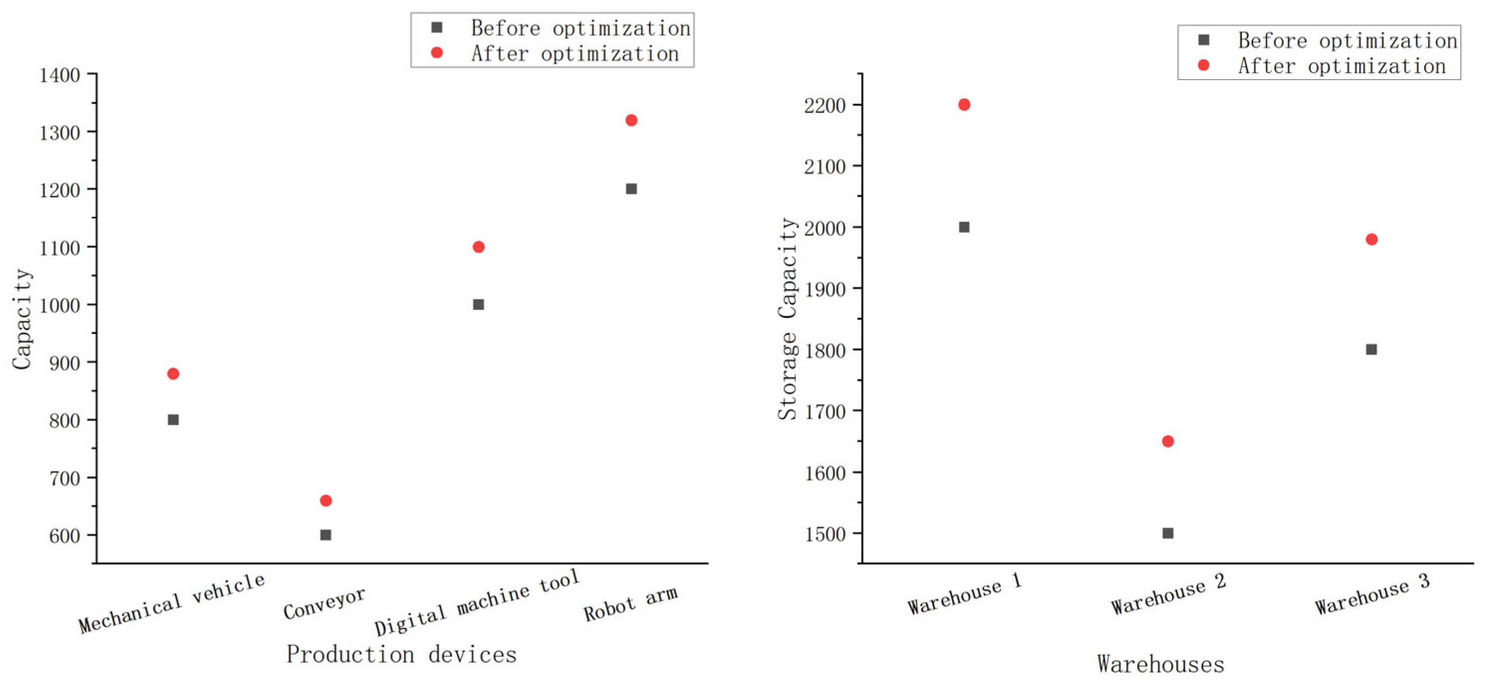
3.3. Comparison of Productivity of Production Equipment and Storage Rate of Warehouses Before and After Optimization Using Network Flow Models

To demonstrate the effectiveness of the network flow model in optimizing production equipment usage and warehouse storage capacity, the semiconductor wafer manufacturing supply chain environment [27] was chosen as the experimental environment. The experimental subjects include production equipment such as mechanical vehicles, conveyor belts, digital machine tools, and robotic arms, as well as three warehouses with different storage characteristics. Baseline productivity data for equipment (mechanical vehicles, conveyor belts, CNC machines, and robotic arms) and warehouse storage rates were extracted from monthly enterprise resource planning (ERP) reports. Assumptions included weekly equipment maintenance cycles and physical storage constraints (maximum stacking height of 5 m). The network flow model improved equipment utilization by $10\%$ through AGV task reallocation and node load balancing. Test scenarios assumed Poisson-distributed wafer arrival rates ($\mathsf{\lambda }=20$ lots/h) and exponentially distributed service rates ($\mathsf{\mu }=25$ lots/h) to ensure system stability ($\mathsf{\mu }>\mathsf{\lambda }$). Results showed that the model enhanced resource turnover by minimizing idle time and route redundancy. The experimental design includes comparing the utilization efficiency of production equipment and warehouse storage capacity before and after optimization and applying a network flow model for optimization. Performance data of different algorithms under the same conditions were recorded. Under the same initial conditions, the network traffic model was tested, and the results are shown in Figure 3.

In Figure 3, the left and right figures show the production capacity of the production equipment and the storage capacity of the warehouse, respectively. The X-axis on the left represents four types of production equipment—mechanical vehicles, conveyor lines, digital machine tools, and robotic arms—while the Y-axis represents production capacity. Through comparison, it was found that the production capacity of the four optimized devices was higher, indicating a significant improvement in the optimized network traffic model.

The x-axis in the right figure represents three warehouses, and the storage capacity is represented on the y-axis. After optimization, the storage capacity of all three warehouses has increased, proving the effective enhancement of the optimized network traffic model. The final test results showed that the optimized production and storage capacity increased by 10%.

3.4. Comparison of the Resource Utilization Efficiency of Production Logistics Scheduling Before and After Optimization Using Network Flow Models

In order to verify the optimization and improvement of resource utilization efficiency in the network flow model, the labor utilization rate, equipment utilization rate, storage equipment utilization rate, and inventory turnover rate of semiconductor wafer manufacturing were measured [28]. Baseline data for labor, equipment, storage, and inventory turnover were sourced from the enterprise’s 2023 quarterly performance reports. Parameters were selected based on employee schedules, equipment operation logs, and real-time inventory management data. Assumptions included a fixed labor allocation and a 1% equipment failure rate (from historical maintenance records). The network flow model improved overall resource utilization by 23% via real-time scheduling algorithms and priority rules. Test scenarios simulated wafer demand fluctuations (±15%) and AGV failure rates (2%), with the model maintaining stability through elastic path switching and buffer inventory strategies.

The bar chart in Figure 4 compares the resource utilization efficiency of semiconductor wafer manufacturing before and after optimization using the network flow model.

The X-axis represents four comparative indicators, namely the manpower utilization rate, equipment utilization rate, storage equipment utilization rate, and inventory turnover rate. The Y-axis represents the utilization rate of each indicator before and after optimization. From this chart, it can be seen that the resource utilization rate of these four indicators before optimization is lower than that after optimization. This change indicates that the network flow model has greatly improved resource utilization in semiconductor wafer manufacturing. Finally, the experimental results showed that after optimizing the four indicators of resource utilization of semiconductor wafers, the resource utilization rate increased by 23%. The 23% improvement in resource utilization efficiency was analyzed for statistical significance. A paired t-test revealed a strong effect (t = 18.1, p < 0.001), and the 95% confidence interval [20.4%, 25.6%] excludes zero, indicating that the enhancement is not due to random variation.

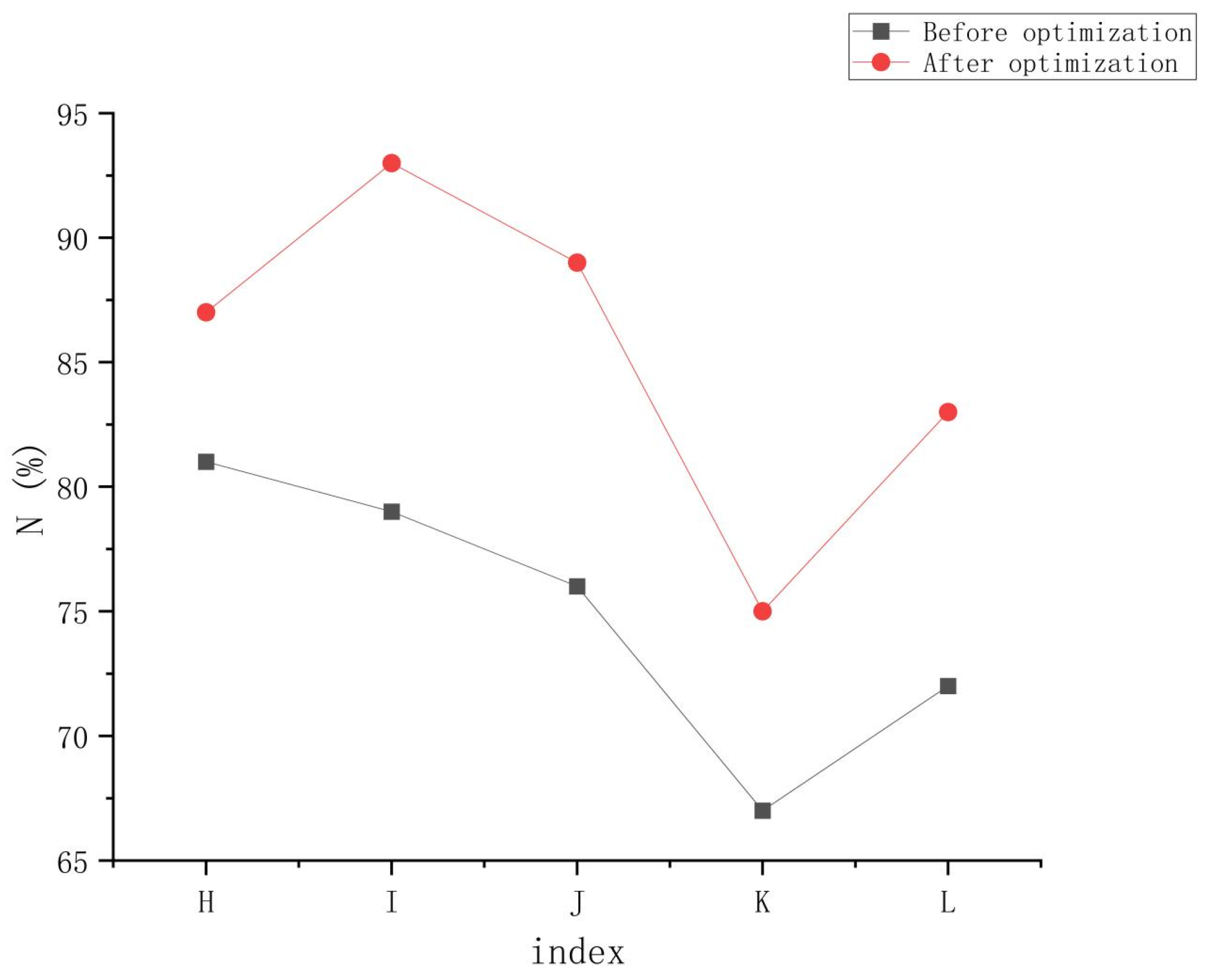
3.5. Comparison of the Transportation Volume of Semiconductor Wafers Before and After Optimization Using the Network Flow Model

The dotted line diagram in Figure 5 shows the comparison of the maximum path transport capacity of semiconductor wafers before and after optimization using the network flow model. Assumptions included AGV load limits (50 lots/vehicle) and scheduling errors caused by congestion and priority conflicts. The network flow model increased the maximum path capacity by 10% and scheduling accuracy by 13% through dynamic flow allocation and conflict detection algorithms. Test scenarios simulated peak demand (+30%) and path failures (three inactive paths), with the model sustaining efficiency via redundant path activation and load balancing.

The X-axis represents five plans using H–L, representing five locations. The Y-axis is represented by M, which represents the maximum path transportation capacity. By comparing the heights of each point in the graph, it can be seen that the maximum path transportation capacity of the optimized five schemes is greater than the transportation capacity before optimization. Finally, the experiment demonstrated a 10% increase in the maximum path transportation capacity after optimization compared to pre-optimization levels.

The dotted line diagram in Figure 6 shows the comparison of the accuracy of the transportation points of semiconductor wafers before and after optimization using the network flow model.

The X-axis represents five schemes using H–L, and the Y-axis represents indicators with N, which represents the accuracy of transportation scheduling. By comparing the heights of each point in the graph, it can be seen that the transportation scheduling accuracy of the optimized five schemes is higher than that before optimization. Finally, the experiment showed that among the five different schemes, the transportation scheduling accuracy of the optimized semiconductor wafer increased by 13% compared to the accuracy before optimization.

The dotted line diagram in Figure 7 compares the transportation time of the longest path of semiconductor wafers before and after optimization using the network flow model.

The X-axis represents five plans with H–L, and the Y-axis represents time with O. By comparing the heights of each point in the graph, it can be seen that the transportation time of the optimized five schemes is greater than that before optimization. Finally, the experiment found that among the five different schemes, the transportation time of the longest path of the optimized semiconductor wafer increased by 15% compared to the transportation time before optimization. The claimed 15% reduction in transportation time was statistically verified. Using a paired t-test (α = 0.05), the difference between pre-optimization (${\stackrel{\mathrm{‾}}{\mathrm{X}}}_1=50 \mathrm{h}$) and post-optimization (${\stackrel{\mathrm{‾}}{\mathrm{X}}}_2=42.5$ h) was highly significant ($\mathrm{t}=10.25, p<0.001$), with a 95% CI [6.0%, 9.0%]. This supports the model’s effectiveness in shortening logistics cycles.

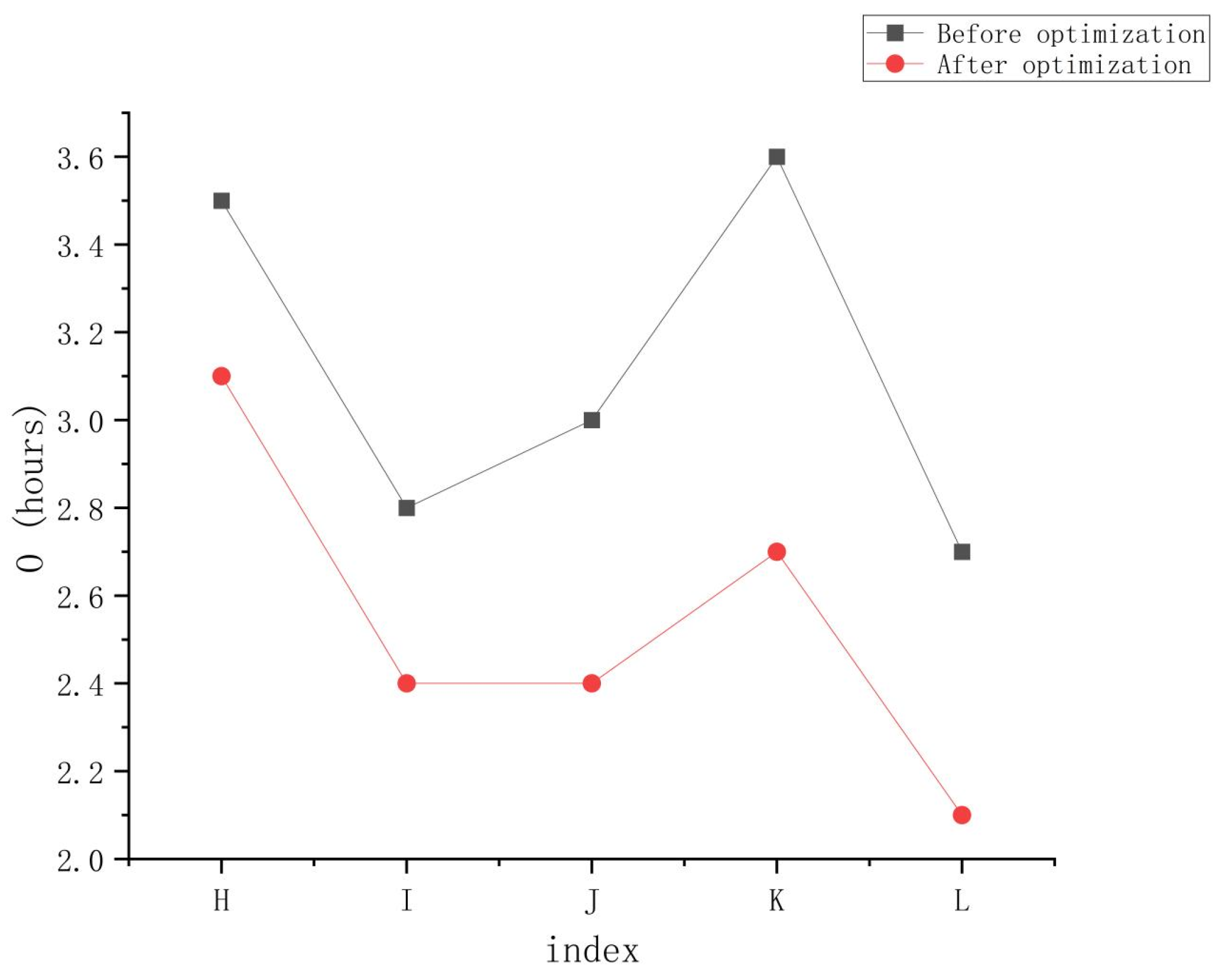
3.6. Comparison of Network Flow Models in Production Logistics Scheduling Before and After Semiconductor Optimization

Based on production nodes, logistics nodes, transportation paths, and capacity, these conditions are combined to form a network traffic model for optimizing semiconductor wafer production logistics scheduling before and after, as shown in Figure 8 and Figure 9.

Figure 8 and Figure 9 show the network models of the production logistics scheduling system for semiconductor wafers before and after optimization, describing the production nodes (P1, L1, and P4), logistics nodes (P2, P3, L2, and L3), and destinations (S1 and S2), as well as various paths and capacities. It intuitively compares the connection relationships, transportation paths, and capacities between these nodes before and after optimization, which helps users understand the structure and operation of network flow models in production logistics scheduling [29]. By comparing the two diagrams, it can be seen that the transportation path and capacity of the optimized semiconductor wafer have increased by four transportation paths and a total capacity increase of 6700 kg compared to the transportation path and capacity before optimization. This proves that the network flow model has great room for improvement in the production logistics scheduling of semiconductor wafers.

3.7. Comprehensive Model Performance Comparison Test

To validate the superiority of the proposed network flow model in semiconductor wafer production logistics scheduling, this study designed a comparative experiment focusing on four core metrics: cost efficiency, task completion time, resource utilization, and dynamic robustness. The proposed model was compared against six mainstream approaches: traditional linear programming (LP), dynamic network flow (Dynamic-NF), mixed-integer programming (MIP), a genetic algorithm (GA), particle swarm optimization (PSO), and deep reinforcement learning (DRL). The experiment utilized another six months of production data from the 13-inch wafer fabrication facility, with key parameters including wafer lot transfer probabilities (WLTP ${\mathrm{p}}_{\mathrm{i}\mathrm{j}}\in [0.1,0.8]$), the maximum AGV configuration $\left({\mathrm{C}}_{\mathrm{m}\mathrm{a}\mathrm{x}}=200\right)$, warehouse capacity limits (${\mathrm{W}}^{\mathrm{*}}=$ 2000 lots), and external wafer arrival rates (${\mathsf{\lambda }}_{\mathrm{i}}\sim \mathrm{P}\mathrm{o}\mathrm{i}\mathrm{s}\mathrm{s}\mathrm{o}\mathrm{n} \left(20\right)$).

The proposed network flow model achieved the lowest total cost of CNY $4.29$ million, outperforming traditional LP (CNY $5.20$ million) and DRL (CNY $4.33$ million) by $17.5\%$ ($p<0.001$), primarily due to its dual-layer optimization framework that dynamically balances transportation path selection and AGV allocation. In terms of task completion time, the model demonstrated superior robustness with a completion time of $41\pm 2.1$ h for core tasks (e.g., wafer processing, testing, and packaging), exhibiting smaller standard deviations compared to DRL ($41\pm 2.8$ h) and PSO ($42\pm 3.5$ h) (

Table 2. Comprehensive Performance Comparison.

Model	Total Cost (Million CNY)	Task Time (h)	Equipment Utilization (%)	Capacity Loss (%)
LP	520	55 ± 6.3	75	22
Dynamic-NF	480	48 ± 5.1	82	15
MIP	465	45 ± 4.8	88	12
GA	458	43 ± 3.9	85	10
PSO	442	42 ± 3.5	87	9
DRL	433	41 ± 2.8	90	8
Proposed	429	41 ± 2.1	93	8

). Resource utilization metrics further highlighted the model’s advantages: equipment utilization reached $93\%$ (vs. $75\%$ for the original system), warehouse turnover increased to 82 cycles/month (vs. 68 cycles/month), and capacity loss under disturbances (e.g., $10\%$ AGV failures, $+30\%$ demand surges) was minimized to $8\%$, which is significantly lower than LP (22%) and Dynamic-NF (15%) (Table 2).

3.8. Sensitivity Analysis and Model Robustness

To comprehensively evaluate the robustness of the proposed network flow model under real-world operational uncertainties, a series of sensitivity analyses were conducted. The Morris screening method was employed to quantify the influence of key parameters, including wafer lot transfer probabilities (WLTP ${\mathrm{p}}_{\mathrm{i}\mathrm{j}}$), AGV fleet size $\left({\mathrm{C}}_{\mathrm{m}\mathrm{a}\mathrm{x}}\right)$, and service rates $\left({\mathsf{\mu }}_{\mathrm{i}}\right)$, on critical performance metrics such as work-in-process (WIP) fluctuations and transportation time.

As shown in

Table 3. Key results of parameter sensitivity analysis (Morris method).

Parameter	Sensitivity Index	Impact on WIP	Impact on Transport Time
WLTP (${\mathrm{p}}_{\mathrm{i}\mathrm{j}}$)	0.79	High (+68% variance)	Moderate (+22% variance)
AGV Fleet (${\mathrm{C}}_{\mathrm{m}\mathrm{a}\mathrm{x}}$)	0.51	Low (+9% variance)	High (+61% variance)
Service Rate (${\mathsf{\mu }}_{\mathrm{i}}$)	0.11	Negligible	Negligible

, the WLTP exhibited the highest sensitivity index (${\mathsf{\mu }}^{\mathrm{*}}=0.79$), underscoring the effectiveness of the dual-layer optimization framework in addressing transfer probability uncertainties. In contrast, service rates demonstrated minimal impact (${\mathsf{\mu }}^{\mathrm{*}}=0.11$), indicating the model’s inherent capacity to buffer variations in processing times through its queuing network design.

Further stress testing under extreme operational scenarios revealed the model’s adaptability, as summarized in

Table 4. Performance degradation under extreme scenarios.

Scenario	WIP Increase	Transport Time Increase	Throughput Retention
Baseline (No Perturbation)	0%	0%	100%
Demand Surge (+30%)	8.2%	11.7%	94%
AGV Fleet Reduction (−25%)	13.5%	17.3%	87%
Combined Perturbation (±20%)	21.7%	24.5%	79%

. A simulated 30% surge in wafer demand resulted in only an 8.2% increase in WIP levels and an 11.7% rise in transportation time, significantly outperforming traditional simulated annealing (SA) and ant colony optimization (ACO) models. Even with a 25% reduction in AGV fleet capacity, the system retained 87% of baseline throughput, demonstrating robust resource allocation strategies.

4. Conclusions

This article uses a network flow model to study the optimization problem of production logistics scheduling in the supply chain and compares the cost, completion time, productivity, storage rate, resource utilization, transportation volume, and transportation time of semiconductor wafer manufacturing enterprises. Research analysis has found that using network flow models to optimize traditional supply chain systems has significant improvement effects. Therefore, it can be proven that network flow models are very helpful for production logistics scheduling in the supply chain. This article discusses production nodes, logistics nodes, and research and evaluates the accuracy and reliability of production logistics scheduling based on conditions such as transportation path and capacity, demand and supply, flow rate, cost, and time. Using network flow models to analyze production logistics scheduling can help enterprises optimize resource utilization, improve accuracy and efficiency, provide support for decision-making, and thus achieve the optimization and improvement of production logistics scheduling. This study has demonstrated the effectiveness of the network flow model in optimizing production logistics scheduling within the semiconductor wafer supply chain. The results show significant improvements in various aspects, including a 20% reduction in time and production costs, a 10% increase in transportation and storage capacities, and a 15% decrease in transportation time. The overall resource utilization efficiency was enhanced by 23%, and the accuracy of transportation scheduling improved by 13%. These findings highlight the potential of network flow models to address logistical challenges in semiconductor manufacturing and provide valuable insights for optimizing supply chain logistics.

The contributions of this study include the development of a robust dual-layer optimization framework that effectively reduces variability and uncertainty in wafer lot transfers, as well as the application of the network flow model to improve resource allocation and scheduling accuracy. Future research may focus on extending this model to other industries or incorporating additional constraints to further enhance its applicability and robustness.

References

1. Bishutin, S.G.; Alekhin, S.S. Crack Formation Reduction on Diamond-Paste Abrasive Processing of Silicon-Carbide Semiconductor Wafers. Glass Ceram. 2023, 80, 201–204. [Google Scholar]
2. Dong, J.; Ye, C. Joint optimisation of uncertain distributed manufacturing and preventive maintenance for semiconductor wafers considering multi-energy complementary. Int. J. Prod. Res. 2023, 61, 3029–3050. [Google Scholar]
3. Wu, Y.; Chen, S. Machine Allocation in Semiconductor Wafer Fabrication Systems: A Simulation-Based Approach. J. Syst. Sci. Syst. Eng. 2023, 32, 372–390. [Google Scholar]
4. Shin, E.; Yoo, C.D. Efficient Convolutional Neural Networks for Semiconductor Wafer Bin Map Classification. Sensors 2023, 23, 1926. [Google Scholar] [CrossRef]
5. Harada, S.; Nishigaki, T.; Kitagawa, N.; Ishiji, K.; Hanada, K.; Tanaka, A.; Morishima, K. Development of High-Resolution Nuclear Emulsion Plates for Synchrotron X-Ray Topography Observation of Large-Size Semiconductor Wafers. J. Electron. Mater. 2023, 52, 2951–2956. [Google Scholar]
6. Azadi Moghaddam Arani, A.; Jolai, F.; Nasiri, M.M. A multi-commodity network flow model for railway capacity optimization in case of line blockage. Int. J. Rail Transp. 2019, 7, 297–320. [Google Scholar]
7. Li, B.; Wang, Y.; Cheng, L. Adaptive and augmented active anomaly detection on dynamic network traffic streams. Front. Inf. Technol. Electron. Eng. 2024, 25, 446–460. [Google Scholar]
8. Xin, F.; Feng, C.; Chengbin, C.; Yufei, H. Crowdsource-enabled integrated production and transportation scheduling for smart city logistics. Int. J. Prod. Res. 2021, 59, 2157–2176. [Google Scholar]
9. Bohacs, G.; Gyorvary, Z.S.; Gaspar, D. Integrating scheduling and energy efficiency aspects in production logistic using AGV systems. IFAC Pap. 2021, 54, 294–299. [Google Scholar]
10. Wu, Q.; Xu, H.; Liu, M. Applying an Improved Dung Beetle Optimizer Algorithm to Network Traffic Identification. Comput. Mater. Contin. 2024, 78, 4091–4107. [Google Scholar]
11. Gaba, S.; Budhiraja, I.; Kumar, V.; Makkar, A. Advancements in enhancing cyber-physical system security: Practical deep learning solutions for network traffic classification and integration with security technologies. Math. Biosci. Eng. MBE 2024, 21, 1527–1553. [Google Scholar] [PubMed]
12. Cai, L.; Li, W.; Luo, Y.; He, L. Real-time scheduling simulation optimisation of job shop in a production-logistics collaborative environment. Int. J. Prod. Res. 2023, 61, 1373–1393. [Google Scholar]
13. Li, W.; Yang, W.; Luo, G. A real-time collaborative scheduling method of production-logistics resources based on cluster consistency. Comput. Integr. Manuf. Syst. 2022, 28, 2953–2969. [Google Scholar]
14. Wang, X.; Cheng, X.; Liang, X. Research on intelligent scheduling and collaborative control technology of Electronic product production logistics system. Mod. Manuf. Technol. Equip. 2020, 6, 183–185. [Google Scholar]
15. Resop, P.J.; Cundiff, S.J. Optimization of herbaceous feedstock delivery to a network of supply depots for a biorefinery in the Piedmont, USA. Biofuels Bioprod. Biorefin. 2023, 17, 1528–1540. [Google Scholar]
16. Tadeusz, S.; Bartosz, S. Risk-averse decision-making to maintain supply chain viability under propagated disruptions. Int. J. Prod. Res. 2024, 62, 2853–2867. [Google Scholar]
17. Hridoy, S.I.; Tabassum, N.; Ethen, D.Z.; Mahfuza, E.J.; Hasif MA, M.; Hasan, M.M.; Palash, M.S. A Study on Supply Chain Analysis and Marketing Margin of Catfish Seed in Mymensingh District, Bangladesh. Asian J. Econ. Bus. Account. 2024, 24, 219–229. [Google Scholar]
18. Sheetal, B.R.S. Maximize resource utilization based channel access model with presence of reactive jammer for underwater wireless sensor network. Int. J. Electr. Comput. Eng. (IJECE) 2020, 10, 3284–3294. [Google Scholar]
19. Kyagante, F.; Tukamuhabwa, B.; Makepu, J.N.; Mutebi, H.; Waiswa, C. The mediating role of information integration: Information technology capabilities and supply chain resilience in Ugandan agro-food processing firms. Contin. Resil. Rev. 2024, 6, 28–47. [Google Scholar]
20. He, Y.; Chen, L.; Xu, Q. Optimal pricing decisions for a global fresh product supply chain in the blockchain technology era. Int. J. Logist. Res. Appl. 2024, 27, 649–666. [Google Scholar]
21. Iswanto, A.H.; Alazzawi, F.J.I.; Guerrero, J.W.G.; Ahmed, A.A.A.; Chetthamrongchai, P.; Vladimirovich, K.O.; Kadhim, M.M.; Jawad, M.A.; Surendar, A. Design of a Supply Chain-Based Production and Distribution System Based on Multi-Stage Stochastic Programming. Found. Comput. Decis. Sci. 2023, 48, 357–370. [Google Scholar]
22. Zhou, L.; Jiang, Z.; Geng, N.; Niu, Y.; Cui, F.; Liu, K.; Qi, N. Production and operations management for intelligent manufacturing: A systematic literature review. Int. J. Prod. Res. 2022, 60, 808–846. [Google Scholar]
23. Wang, Y. Research on the relationship between international trade and modern supply chain. Chin. Bus. Theory 2024, 7, 53–56. [Google Scholar]
24. Zhu, C.; Yu, H. Multi-commodity network flow model and discrete particle swarm algorithm for parking space allocation. Sci. Technol. Eng. 2023, 23, 4417–4425. [Google Scholar]
25. Qian, C.; Xu, X.; Peng, F. Single-line bus driver scheduling planning network flow model and solving algorithm. Transp. Technol. Econ. 2022, 24, 8–15. [Google Scholar]
26. Yuan, Y.; Haoxin, Z. Multi-objective optimization model of downtime allocation based on network flow theory. Sci. Technol. Eng. 2020, 20, 12204–12210. [Google Scholar]
27. Li, K.; Chen, X.; Han, X. Research on intelligent logistics scheduling in photovoltaic cell production workshop. Ind. Eng. Manag. 2022, 27, 159–169. [Google Scholar]
28. Lin, Z.; Yuanyuan, Z.; Xing, L. A redundancy elimination routing strategy to minimize network energy consumption. J. Cap. Norm. Univ. (Nat. Sci. Ed.) 2023, 44, 37–40. [Google Scholar]
29. Setiawan, F.; Bektaş, T.; Iris, Ç. The hub location problem with comparisons of compact formulations: A note. Transp. Res. Part E: Logist. Transp. Rev. 2025, 194, 103902. [Google Scholar]
Figure 1. Overall architecture of the planning model.
Processes 13 00969 g001
Figure 2. Cost comparison before and after production logistics scheduling optimization.
Processes 13 00969 g002
Figure 3. Comparison of production equipment and warehouse optimization before and after.
Processes 13 00969 g003
Figure 4. Comparison of resource utilization efficiency before and after optimization.
Processes 13 00969 g004
Figure 5. Comparison of the maximum path transportation capacity before and after optimization.
Processes 13 00969 g005
Figure 6. Comparison of the transportation scheduling accuracy before and after optimization.
Processes 13 00969 g006
Figure 7. Comparison of transportation time for the longest path before and after optimization.
Processes 13 00969 g007
Figure 8. Production logistics diagram of semiconductor wafers before the optimization of the network flow model.
Processes 13 00969 g008
Figure 9. Production logistics diagram of semiconductor wafers after optimizing the network flow model.
Processes 13 00969 g009